The Geneva-Copenhagen Survey of the Solar neighbourhood II

Abstract

Context. Ages, metallicities, space velocities, and Galactic orbits of stars in the Solar neighbourhood are fundamental observational constraints on models of galactic disk evolution. Understanding and minimising systematic errors and sample selection biases in the data is crucial for their interpretation.

Aims. We aim to consolidate the calibrations of uvby$\beta$ photometry into $\rm T_{eff}$, [Fe/H], distance, and age for F and G stars and rediscuss the results of the Geneva-Copenhagen Survey (Nordström et al. 2004; GCS) in terms of the evolution of the disk.

Methods. We use recent V-K photometry, angular diameters, high-resolution spectroscopy, Hipparcos parallaxes, and extensive numerical simulations to re-examine and verify the temperature, metallicity, distance, and reddening calibrations for the uvby$\beta$ system. We also highlight the selection effects inherent in the apparent-magnitude limited GCS sample.

Results. We substantially improve the $\rm T_{eff}$ and [Fe/H] calibrations for early F stars, where spectroscopic temperatures have large systematic errors. A slight offset of the GCS photometry and the non-standard helium abundance of the Hyades invalidate its use for checking metallicity or age scales; however, the distances, reddenings, metallicities, and age scale for GCS field stars require minor corrections only. Our recomputed ages are in excellent agreement with the independent determinations by Takeda et al. (2007), indicating that isochrone ages can now be reliably determined.

Conclusions. The revised G-dwarf metallicity distribution remains incompatible with closed-box models, and the age-metallicity relation for the thin disk remains almost flat, with large and real scatter at all ages ($\sigma_{intrinsic}$= 0.20 dex). Dynamical heating of the thin disk continues throughout its life; specific in-plane dynamical effects dominate the evolution of the $U$ and $V$ velocities, while the $W$ velocities remain random at all ages. When assigning thick and thin-disk membership for stars from kinematic criteria, parameters for the oldest stars should be used to characterise the thin disk.

1 Introduction

Models for the evolution of spiral galaxy disks describe their star formation history, nucleosynthesis, chemical enrichment, and dynamical evolution. Traditional parameterised models yield single-valued relations for the increase in the (total or individual) heavy-element abundances of stars at a given position in the disk, radial gradients in elemental abundances, and the kinematic heating of the local disk, all as functions of time. The underlying paradigm is the efficient mixing and recycling of interstellar gas, such that mean values of abundances and kinematics as functions of time and radial position in the disk describe the underlying physical processes adequately (see Casuso & Beckman casuso04 (2004), Naab & Ostriker naab06 (2006), or Cescutti at al. cescutti07 (2007) for recent examples). Any dispersion of the observed values around the mean relations is assumed to be due to observational error.

Under realistic conditions, however, local variations in the rate of chemical enrichment must have occurred (see e.g. Brook et al. brook07 (2007) for such an approach). The question of interest is therefore how well these relations and their intrinsic scatter can be determined from the observations.

The Milky Way is the one galaxy in which these predictions can be tested in detail. Thus, complete, accurate information on the stellar content of the Solar neighbourhood remains a fundamental observational constraint on any set of models. Much of the discussion focuses on the age-metallicity relation (AMR) for the Solar neighbourhood, and the key questions are two-fold (Twarog twarog (1980), Carlberg et al. carlberg (1985), Meusinger, Stecklum & Reimann meusinger (1991), Edvardsson et al. edv93 (1993), Rocha-Pinto et al rocha-pinto00 (2000), Feltzing, Holmberg & Hurley feltzing01 (2001), and Nordström et al. nordstrom04 (2004)): (i) Does the average relation show the expected rise in metallicity from the formation of the (thin) disk to the present time? and (ii) how large is the intrinsic dispersion in metallicity at any given age? Given the wide-ranging ramifications of these questions, the observational data used for the test must be prepared, selected, and discussed with the utmost care.

The most comprehensive recent study of nearby stars in the solar neighbourhood is the Geneva-Copenhagen Survey (Nordström et al. nordstrom04 (2004); GCS in the following). The GCS provides metallicities, ages, kinematics, and Galactic orbits for a complete, magnitude-limited, all-sky sample of $\sim$14,000 F and G dwarfs brighter than $V\sim 8.3$. The basic observational data are uvby$\beta$ photometry, Hipparcos/Tycho-2 parallaxes and proper motions, and some 63,000 new, accurate radial velocity observations, supplemented by earlier data. The best calibrations then available were used to derive $\rm T_{eff}$, [Fe/H], and distances from the photometry. The astrometry and radial velocities were then used to compute space motions and identify binaries in the sample. Finally, unbiased ages and error estimates were computed from a set of theoretical isochrones by a sophisticated Bayesian technique (Jørgensen & Lindegren jorgensen05 (2005)), and Galactic orbits were computed from the present positions and velocity vectors of the stars and a Galactic potential model.

The GCS is large enough to yield adequate statistics for subsets of stars defined by age, metallicity, or abundance, and is essentially free of the kinematic and/or metallicity biases affecting most earlier samples. However, systematic selection effects may still remain in the data or be introduced by the calibrations used to derive astrophysical parameters from the observations. Accordingly, the purpose of the present paper is to critically re-examine the observational determination of $\rm T_{eff}$, [Fe/H], and age for F- and G-type dwarf stars in the light of the most recent developments in the field. We also compare our results with those of the recent papers by Haywood (haywood06 (2006); H06 in the following), Valenti & Fischer (valenti (2005); VF05 in the following), and Takeda et al. (takeda (2007)).

We begin the paper by briefly describing the possible impact of systematic and random errors in these parameters on the overarching theme of spiral galaxy evolution in Sect. 2. The reader mostly interested in our new uvby$\beta$ calibrations in terms of effective temperature, metallicity, distance, reddening, and age computations will find these discussed in Sect. 3 – 7. The reader primarily interested in the evolution of the Galactic disk may skip directly to Sect. 8, where we discuss the end-to-end simulations we have used to verify the robustness of the results reached with the new calibrations. We rediscuss the “G dwarf problem”, age-metallicity, and age-velocity relations for the Solar neighbourhood in Sect. 9 – 11 and compare the thick and thin disks in Sect. 12. Finally, we summarise our findings and conclusions in Sect. 13.

2 Astrophysical implications of calibration errors

The key parameters to be compared with models are the masses (i.e. main-sequence lifetimes), ages, heavy-element abundances, spatial distributions, and space velocities or Galactic orbits for sufficiently large samples of stars that are representative of the general population of disk stars. However, except for positions and velocities, these parameters cannot be determined by direct observation.

Typical observational data are multiband colour indices and perhaps spectra, from which $\rm T_{eff}$, [Fe/H], and absolute magnitude or log $g$ are derived, using theoretical or empirical calibrations. From $\rm T_{eff}$, [Fe/H], and $\rm M_{V}$, in turn, the age and mass of each star can be derived by comparison with stellar models.

This is straightforward in theory. In practice, it is highly non-trivial because the problem is very non-linear, and significant uncertainties in the calibrations remain. In particular, uncertainties in the theory of stellar atmospheres continue to play a major role, both for the predicted effective temperatures of stellar models and for the transformations between $\rm T_{eff}$, [Fe/H], and log $g$ and the observed colour indices. Because of the strong correlations between these parameters, calibration errors in one may bias the determination of another and lead to spurious correlations between the derived quantities, and incorrect conclusions about the evolution of the Galactic disk.

As one example, assume that the adopted calibration yields too high $\rm T_{eff}$ for the hotter stars (as indeed we find below). [Fe/H] as determined from equivalent widths of spectral lines will then be overestimated. The hotter $\rm T_{eff}$ corresponds to a lower age, the higher [Fe/H] to cooler models and thus an even lower derived age for the observed star. A spurious age-metallicity relation results.

As another example, assume that the $\rm T_{eff}$ scale of the models is correct for the solar abundance, but too hot at lower [Fe/H], as was found in GCS. This will lead to overestimated ages for the metal-poor stars, i.e. again a spurious age-metallicity relation. A similar – or additional – error is introduced if the enhanced [$\alpha$/Fe] ratio of metal-poor stars (e.g. Edvardsson et al. edv93 (1993)) is ignored; if the heavy-element abundance parameter $Z$ of the models is assumed to scale simply as [Fe/H], too hot models are selected, and the resulting age is overestimated again.

Finally, the importance of a clear understanding of the definition of the stellar sample cannot be over-emphasised: Taking the AMR as the prototype again, the choice of stellar sample can determine the outcome even before a single observation is made. E.g., the F-dwarf sample studied by Edvardsson et al. (edv93 (1993)) excluded any old, metal-rich stars that might exist and a priori decided the shape of their AMR - a fact emphasised in the paper, but largely ignored in later references. More complete and accurate observational data are always useful, but temperature calibrations, the choice and verification of stellar models, and the methods used to compute ages and their uncertainties are far more urgent issues at present.

3 Temperature calibration

$\rm T_{eff}$ is the most critical parameter in the determination of isochrone ages, but also affects the spectroscopic metallicity determinations. Two qualitatively different methods to determine $\rm T_{eff}$ exist, based on measurements of spectral lines or on colour indices. When using spectra, the determination of $\rm T_{eff}$ is usually based on the excitation balance of iron, but depth ratios of sets of spectral lines have also been used. When using photometry, the determination of $\rm T_{eff}$ is usually tied to the infrared flux of the stars as estimated from models (the IRFM technique).

For a fundamental test, we return to the basic definition of $\rm T_{eff}$: $f_{\rm bol}=\frac{\phi^{2}}{4}\sigma T_{\rm eff}^{4}$, where $f_{\rm bol}$ is the bolometric flux and $\phi$ the angular diameter of the star. The practical problem in applying the formula is that solar-type main-sequence stars have very small angular diameters that are difficult to measure accurately. The situation is quickly improving, however, as new interferometers enter operation, notably the ESO VLTI. Kervella et al. (kervella04 (2004)) summarise the situation and give diameters for 20 A-M main-sequence stars and 8 A-K0 sub-giants. The angular diameters are of excellent quality, especially those from the VLTI, which have errors down to 1%.

Ramírez & Meléndez (2005a ) combined these diameters with bolometric flux measurements to derive $\rm T_{eff}$ directly for 10 dwarfs and 2 sub-giants. Propagating the errors in the diameters and fluxes through to the temperatures, the mean error is 57K. Ramírez & Meléndez (2005a ) also give (IRFM) estimates for these stars, with a mean difference $<T_{\rm eff}^{\rm IRFM}-T_{\rm eff}^{\rm dir}>$= 10K, dispersion 98K, and mean error 28K.

As regards spectroscopic $\rm T_{eff}$ determinations, Santos et al. (santos05 (2005) and references therein) give results for stars both with and without detected planetary companions, including 7 stars with measured angular diameters. The mean difference is $<T_{\rm eff}^{\rm Santos}-T_{\rm eff}^{\rm dir}>$= 92K, with a dispersion of 91K and mean error 34K. This is in agreement with Santos et al. (santos05 (2005)) themselves, who find their $\rm T_{eff}$ scale to be 139K hotter than that by Alonso et al. (alonso96 (1996)), based on the IRFM and calibrated to B-V and [Fe/H].

Another valuable comparison is with the recent paper by VF05. They give spectroscopic data for $\sim$1000 stars on the Keck/Lick/AAT planet search program, based on fits of synthetic spectra to their high-resolution data and correcting their zero-points from observations of Vesta as a proxy for the Sun. For the 8 stars with measured diameters, the mean difference is $<T_{\rm eff}^{\rm V\&F}-T_{\rm eff}^{\rm dir}>$= 64K, with a dispersion of 124K and mean error 44K.

The reasons for the failure of spectroscopic $\rm T_{eff}$ determinations based on the excitation equilibrium in 1D static LTE models are given in e.g. Asplund (asplund (2005)). Basically, because real stars are spherical, hydrodynamical systems with lines formed in NLTE, the three fundamental assumptions underlying traditional model atmospheres are inadequate and lead to biased results. The correction procedure used by VF05 seems to have eliminated at least part of this bias.

In the following, we review the GCS and other recent temperature scales and derive an improved calibration for the uvby$\beta$ system.

3.1 $\rm T_{eff}$ in the GCS

The marked offset of the Santos et al. (santos05 (2005)) $\rm T_{eff}$ values is confirmed for the 160 stars common to Santos et al. and the GCS, which employed temperatures based on the Alonso et al. (alonso96 (1996)) calibration of b-y, $m_{1}$ and $c_{1}$ to the IRFM scale. The mean difference is $<T_{\rm eff}^{\rm Santos}-T_{\rm eff}^{\rm GC}>$= 127K (dispersion 84K, mean error 7K). For the spectral type range in question, this shows that the GCS $\rm T_{eff}$ scale is in excellent agreement in the mean with temperatures derived directly from the definition of $\rm T_{eff}$.

However, the Alonso et al. (alonso96 (1996)) calibration of b-y, $m_{1}$ and $c_{1}$ may be valid only in the ranges in $\rm T_{eff}$ within which enough calibration stars exist. Fig. 11a of Alonso et al. (alonso96 (1996)) shows the fitted temperatures as a function of b-y and makes clear that there is a marked dearth of calibration stars blueward of b-y $\approx$ 0.3 or $\rm T_{eff}$ $\approx$ 6500K; a similar lack is seen for the reddest stars. Alonso et al. (alonso96 (1996)) give a dispersion for their relation of $\sigma(\theta_{\rm eff})=0.019$ (110K), while Ramírez & Meléndez (2005b ) give 87K for their new b-y relation, albeit at the price of not being valid over the whole parameter range of the GCS stars.

The potential problem in the Alonso et al. (alonso96 (1996)) uvby calibration for blue and red stars is clearly demonstrated by a comparison with other calibrations of Strömgren photometry. They all agree rather well between 0.3$<$b-y$<$0.6, but diverge outside these limits, see e.g. Fig. 24 in Clem et al. (clem04 (2004)).

The situation is unfortunately similar for stars with direct $\rm T_{eff}$ determinations, where Kervella et al. (kervella04 (2004)) have only one star between 6000 and 8500K (Procyon at 6500K), compared to 5 stars between 8500 and 10000K and 11 between 5000 and 6000K.

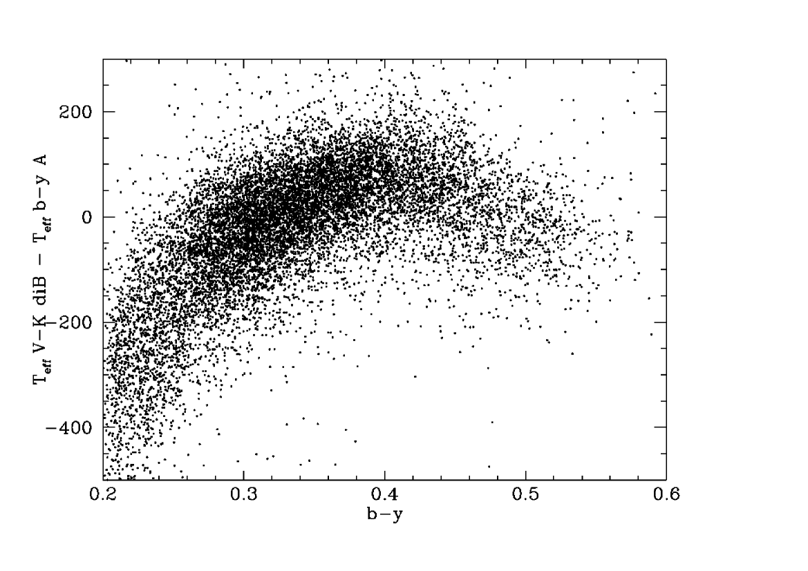
Figure 1: Differences between $\rm T_{eff}$ from the Alonso et al. (alonso96 (1996)) b-y calibration, used in the GCS, and $\rm T_{eff}$ as derived from the V-K calibration by di Benedetto (diBenedetto (1998)).

3.2 Calibrations based on V-K

Alternatively, temperatures based on V-K can be used, because 2MASS photometry is available and well suited to our colour and magnitude ranges: Of the 16682 GCS stars, 16139 have 2MASS K-magnitudes of the highest quality class “A”. We combine these with the $V$ magnitude from the GCS uvby$\beta$ photometry.

In contrast to calibrations based on only visible colours, $\rm T_{eff}$ estimates based on V-K are remarkably robust; the small differences are probably mostly related to the different existing definitions of the K-band. As an example, the V-K calibrations of Alonso (alonso96 (1996)), Ramírez & Meléndez (2005b ), and di Benedetto (diBenedetto (1998)) agree pairwise to within $\sim$20K for the stars in the GCS. In contrast, the Alonso V-K and b-y calibrations differ by 180K rms!

Today, the K-band system of choice is that defined by the 2MASS catalogue, which also gives K magnitudes of high quality for most of the stars in the GCS. We have used the calibration of di Benedetto (diBenedetto (1998)), which is in excellent agreement with the IRFM temperature scale of Ramírez & Meléndez (2005a ) and is valid for the whole colour range of the GCS. In order to transform the Johnson V-K colours used by di Benedetto to the Ks system used by 2MASS, we use the relation:

$$(V-K)_{J}=1.007[(V-K_{s}-0.044)-0.01]$$

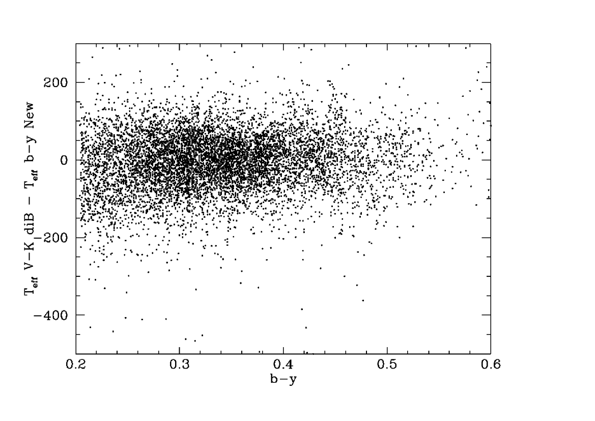
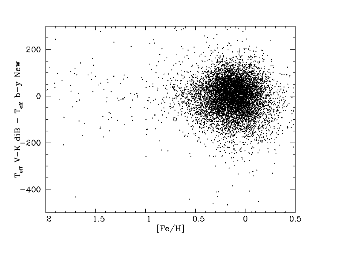
Figure 2: Differences between the $\rm T_{eff}$ of GCS stars as derived from our new b-y calibration and from the V-K calibration by di Benedetto (diBenedetto (1998)).

Fig. 1 shows the difference between the $\rm T_{eff}$ values from the original GCS catalogue and those derived from the 2MASS photometry and the corresponding calibration by di Benedetto (diBenedetto (1998)). The systematic differences are quite marked, especially for the hotter stars.

The trend seen in Fig. 1 is qualitatively similar to that found by H06 (Fig. 7), also by comparison with values from di Benedetto (diBenedetto (1998)), but is better determined here, due to our much larger sample and because V-K is a much more reliable temperature indicator than B-V.

3.3 A new b-y – $\rm T_{eff}$ calibration

Because of the larger number of suitable calibration stars available, the V-K calibration has less systematic error. However, the observational accuracy of the b-y index is substantially better than that of V-K. We have therefore derived a new $\rm T_{eff}$ calibration for b-y, based on the V-K temperature scale set by di Benedetto (diBenedetto (1998)). The best result is achieved when the sample is divided into three temperature ranges. In the blue range (0.20$<$b-y$<$0.33) the relation is:

${\rm\theta_{eff}}=0.649+0.095(b-y)+0.034{\rm[Fe/H]}+1.207(b-y)^{2}\\ \leavevmode\nobreak\ \leavevmode\nobreak\ \leavevmode\nobreak\ \leavevmode\nobreak\ \leavevmode\nobreak\ \leavevmode\nobreak\ \leavevmode\nobreak\ \leavevmode\nobreak\ \leavevmode\nobreak\ -0.005{\rm[Fe/H]}^{2}-0.181(b-y){\rm[Fe/H]}$

where $\rm\theta_{eff}$ = 5040K/$\rm T_{eff}$. The dispersion of the fit is $\rm\sigma(\theta_{eff})=0.007$ when 2.5-$\sigma$ outliers are removed, corresponding to 60K or 0.004 in $\rm\log T_{eff}$ for the mean $\rm\log T_{eff}$.

In the middle range (0.33$<$b-y$<$0.50), the relation is:

${\rm\theta_{eff}}=0.754-0.365(b-y)-0.001{\rm[Fe/H]}+1.635(b-y)^{2}\\ \leavevmode\nobreak\ \leavevmode\nobreak\ \leavevmode\nobreak\ \leavevmode\nobreak\ \leavevmode\nobreak\ \leavevmode\nobreak\ \leavevmode\nobreak\ \leavevmode\nobreak\ \leavevmode\nobreak\ -0.011{\rm[Fe/H]}^{2}-0.091(b-y){\rm[Fe/H]}$

The dispersion of the fit is $\rm\sigma(\theta_{eff})=0.009$ when 2.5-$\sigma$ outliers are removed, corresponding to 57K or again 0.004 in $\rm\log T_{eff}$ for the mean $\rm\log T_{eff}$.

In the red range (0.50$<$b-y$<$0.60), the relation is:

${\rm\theta_{eff}}=0.255+1.656(b-y)+0.018{\rm[Fe/H]}-0.397(b-y)^{2}\\ \leavevmode\nobreak\ \leavevmode\nobreak\ \leavevmode\nobreak\ \leavevmode\nobreak\ \leavevmode\nobreak\ \leavevmode\nobreak\ \leavevmode\nobreak\ \leavevmode\nobreak\ \leavevmode\nobreak\ -0.011{\rm[Fe/H]}^{2}-0.101(b-y){\rm[Fe/H]}$

The dispersion of the fit is $\rm\sigma(\theta_{eff})=0.012$ when 2.5-$\sigma$ outliers are removed, corresponding to 55K or 0.005 in $\rm\log T_{eff}$ for the mean $\rm\log T_{eff}$

We note that this calibration yields 5777K for the Sun when using (b-y)_⊙= 0.403 from Holmberg, Flynn & Portinari (holmberg06 (2006)), although this was not forced on the fit. The two main calibrations are also very well connected: At their common colour, (b-y)= 0.33, the difference in temperature is 2, 6, and 7K at [Fe/H]= 0, -0.50, and -1.00. Due to the small number of very red calibration stars, the difference in $\rm T_{eff}$ grows to -19, 18, and 52K at [Fe/H]= 0, -0.50, and -1.00 at (b-y)= 0.50 – still very small.

Fig. 2 demonstrates the agreement of the resulting $\rm T_{eff}$ values with those derived from V-K and the di Benedetto (diBenedetto (1998)) calibration.

Finally, we compare our new photometric temperatures to the spectroscopic results by VF05. Fig. 3 shows the temperature differences for the 697 single stars in common with the GCS. The mean difference is similar to that from the stars with angular diameters: $<T_{\rm eff}^{\rm V\&F}-T_{\rm eff}^{\rm b-y}>$= 43K, with a dispersion of 91K.

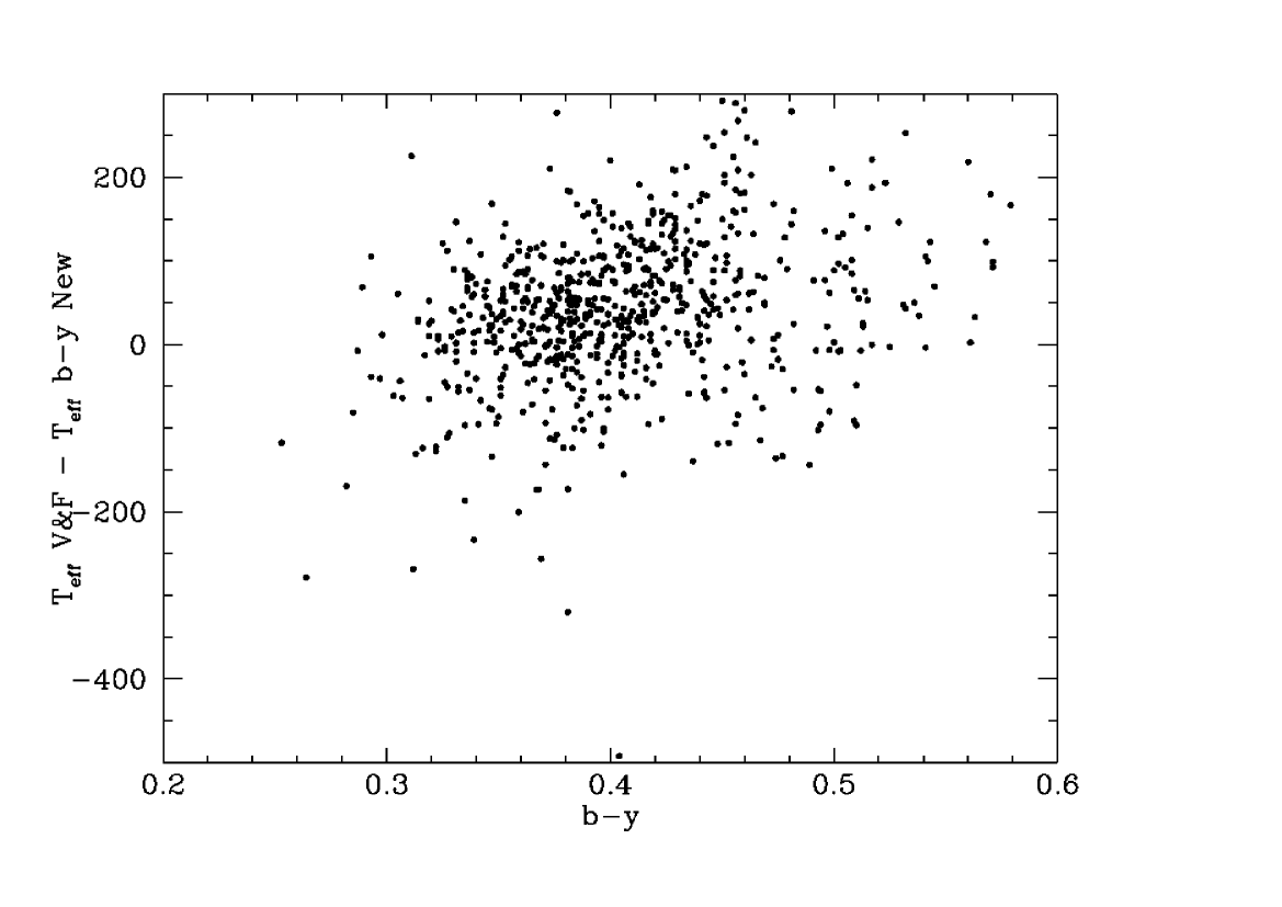
Figure 3: Differences between $\rm T_{eff}$ from our new b-y calibration and $\rm T_{eff}$ as derived from spectrum fitting by VF05.

4 Metallicity calibration

[Fe/H] is important, both in itself as a diagnostic of the chemical evolution of the disk, and because it enters into the determination of stellar ages from theoretical isochrones. However, a comparison of the GCS photometric metallicities with the several high-quality spectroscopic studies available today (Fig. 4) shows significant differences, even when considering only spectroscopic studies using a photometric temperature scale.

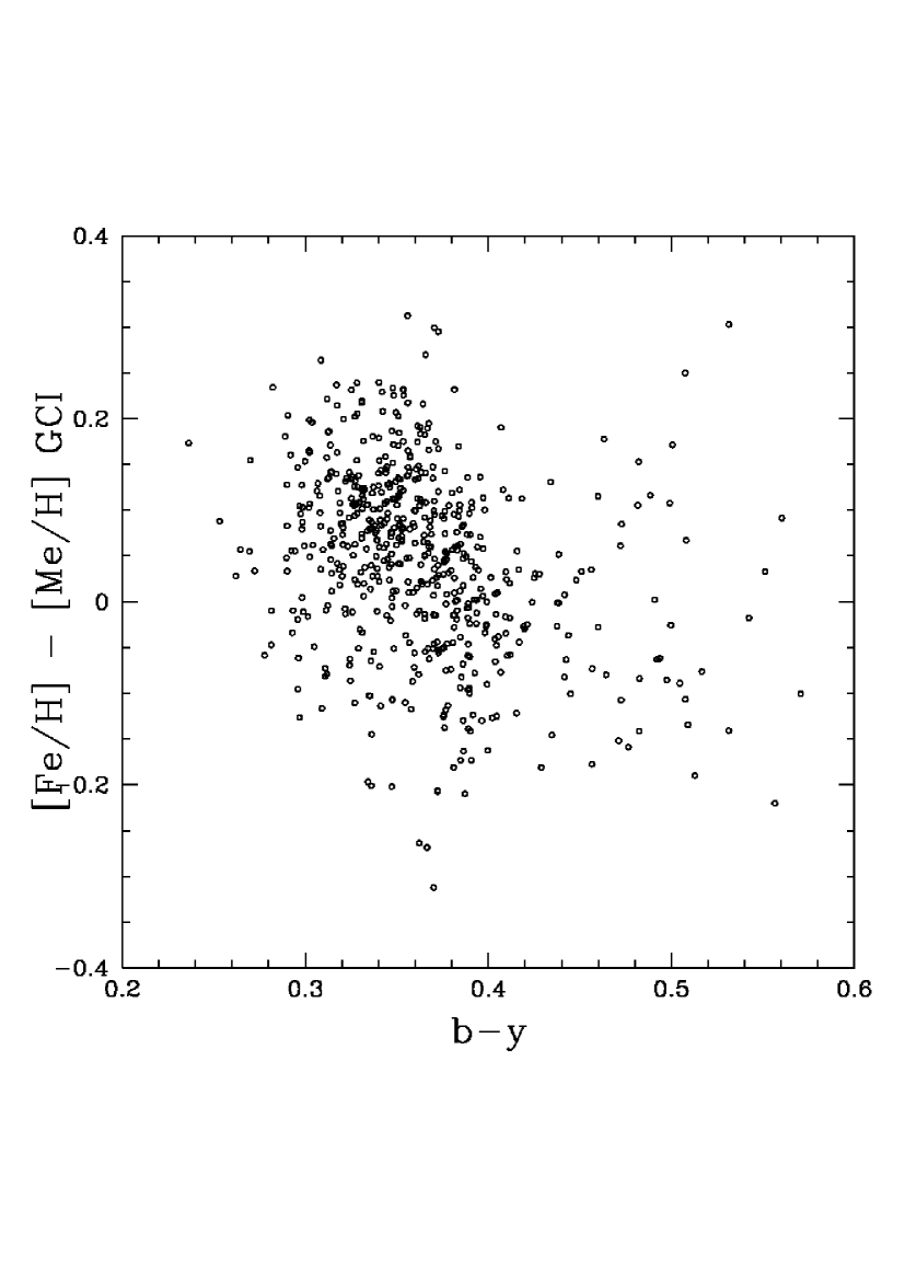
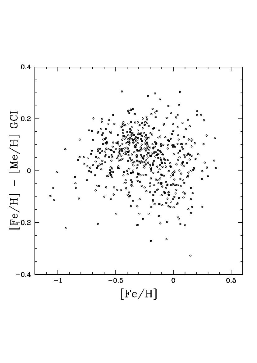
Figure 4: Modern spectroscopic [Fe/H] determinations vs. the photometric [Me/H] of the GCS catalogue.

For the four major spectroscopic studies (in the order Edvardsson et al. edv93 (1993), Chen et al. chenyq00 (2000), Reddy et al. reddy03 (2003), and Allende Prieto et al. allende04 (2004)), the mean differences $<[\rm Fe/H]-[Me/H]>$ are, for the F-calibration range: 0.064, 0.038, 0.114 and 0.013; and for the G-calibration range: 0.019, -0.038, 0.022 and -0.044. Only Allende Prieto et al. (allende04 (2004)) have stars in the range of the “K” calibration (as defined in GCS), with $<[\rm Fe/H]-[Me/H]>$= -0.005.

As regards Santos et al. (santos05 (2005)), who use a spectroscopic $\rm T_{eff}$ scale, we find $<[\rm Fe/H]-[Me/H]>$= 0.162 for stars in F range, $<[\rm Fe/H]-[Me/H]>$= 0.082 for stars in the G range, and $<[\rm Fe/H]-[Me/H]>$= 0.022 for their stars in the K range. We conclude that metallicities derived using the spectroscopic $\rm T_{eff}$ scale must be reduced by about 0.10, 0.09 and 0.03 dex for the F, G and K temperature ranges. This is in fair agreement with the estimated effect on [Fe/H] of a temperature shift of about 100K (see e.g. Feltzing & Gustafsson feltz98 (1998)).

We conclude that, when comparing metallicity scales from different sources, it is crucial to verify how these scales are established. It is especially important to check which $\rm T_{eff}$ scale is used, because an erroneous $\rm T_{eff}$ scale can introduce large biases in the abundances, especially for solar or somewhat hotter temperatures.

4.1 The original GCS calibration

The determination of accurate metallicities for F and G stars is one of the strengths of the Strömgren uvby$\beta$ system. Among the then available uvby$\beta$ calibrations, the GCS used that by Schuster & Nissen (schuni89 (1989)) for the majority of the stars.

However, this calibration was found to give substantial systematic errors for the very reddest G and K dwarfs ($b-y>$ 0.46), where very few spectroscopic calibrators were available at that time. In the GCS we therefore derived a new relation, based on a sample of 72 dwarf stars in the colour range 0.44 $\leq b-y\leq$ 0.59, using the same terms in the calibration equation as the Schuster & Nissen (schuni89 (1989)) G-star calibration. The resulting equation was:

${\rm[Fe/H]}=-2.06+24.56m_{1}-31.61m_{1}^{2}-53.64m_{1}(b-y)\\ \leavevmode\nobreak\ \leavevmode\nobreak\ \leavevmode\nobreak\ +73.50m_{1}^{2}(b-y)+[26.34m_{1}-0.46c_{1}-17.76m_{1}^{2}]c_{1}$

The metallicities from this calibration are compared to the new spectroscopic reference values in Fig. 5. The dispersion around the (zero) mean is 0.12 dex.

For the $\sim$600 stars in the interval 0.44$<$b-y$<$ 0.46, the new calibration agreed with that by the Schuster & Nissen (schuni89 (1989)) to within 0.00 dex in the mean (s.d. 0.12).

About 2400 GCS stars with high $\rm T_{eff}$ and low log $g$ were outside the range covered by the Schuster & Nissen (schuni89 (1989)) calibration. For these stars, the calibration of $\beta$ and $m_{1}$ by Edvardsson et al. (edv93 (1993)) was used when valid. For the stars in common, the two calibrations agree very well (mean difference of 0.00 dex, dispersion only 0.05).

For stars outside the limits of both calibrations, we derived a new relation, using the same terms in the equation as the Schuster & Nissen (schuni89 (1989)) calibration for F stars. From 342 stars in the ranges: 0.18 $\leq b-y\leq$ 0.38, 0.07 $\leq m_{1}\leq$ 0.26, 0.21 $\leq c_{1}\leq$ 0.86, and - 1.5 $\leq[\rm Fe/H]\leq$ 0.8, we found the following calibration equation:

${\rm[Fe/H]}=9.60-61.16m_{1}+81.25m_{1}(b-y)\\ \leavevmode\nobreak\ \leavevmode\nobreak\ \leavevmode\nobreak\ \leavevmode\nobreak\ \leavevmode\nobreak\ \leavevmode\nobreak\ \leavevmode\nobreak\ \leavevmode\nobreak\ \leavevmode\nobreak\ +224.65m_{1}^{2}(b-y)-153.18m_{1}(b-y)^{2}\\ \leavevmode\nobreak\ \leavevmode\nobreak\ \leavevmode\nobreak\ \leavevmode\nobreak\ \leavevmode\nobreak\ \leavevmode\nobreak\ \leavevmode\nobreak\ \leavevmode\nobreak\ \leavevmode\nobreak\ +[12.23-90.23m_{1}+38.70(b-y)]\log(m_{1}-c_{3}),$

where $c_{3}=0.45-3.98(b-y)+5.08(b-y)^{2}$. The dispersion of the fit is 0.10 dex.

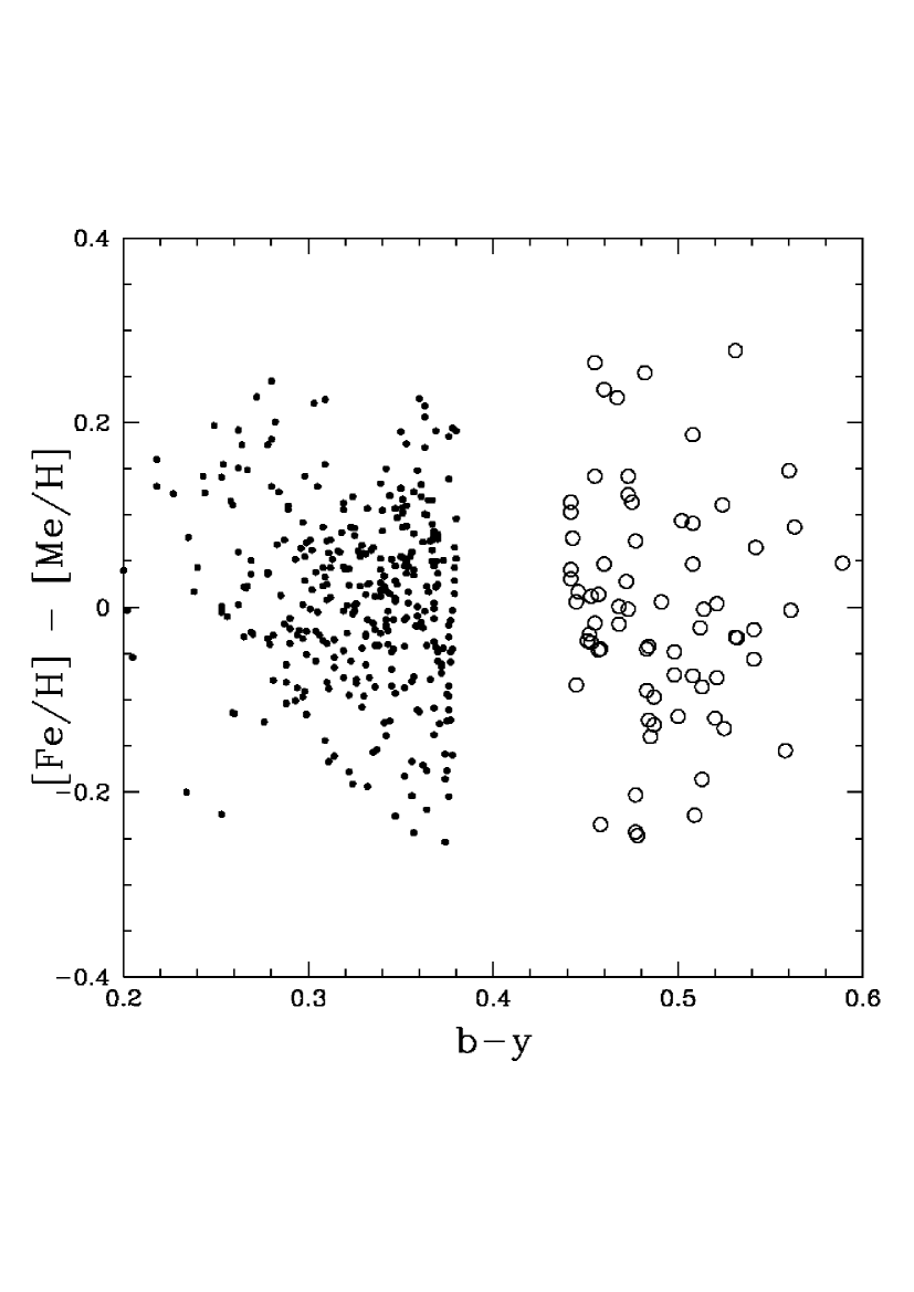
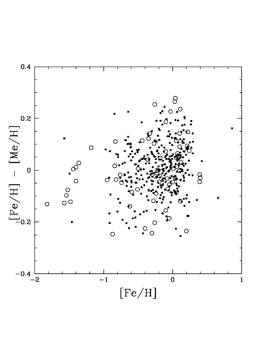
Figure 5: GCS photometric metallicities ([Me/H]) vs. the spectroscopic [Fe/H] values used to establish the calibrations. Open circles depict the cool stars, dots the hot stars (see text).

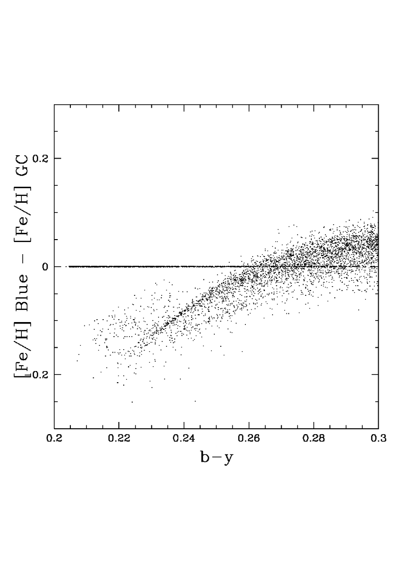
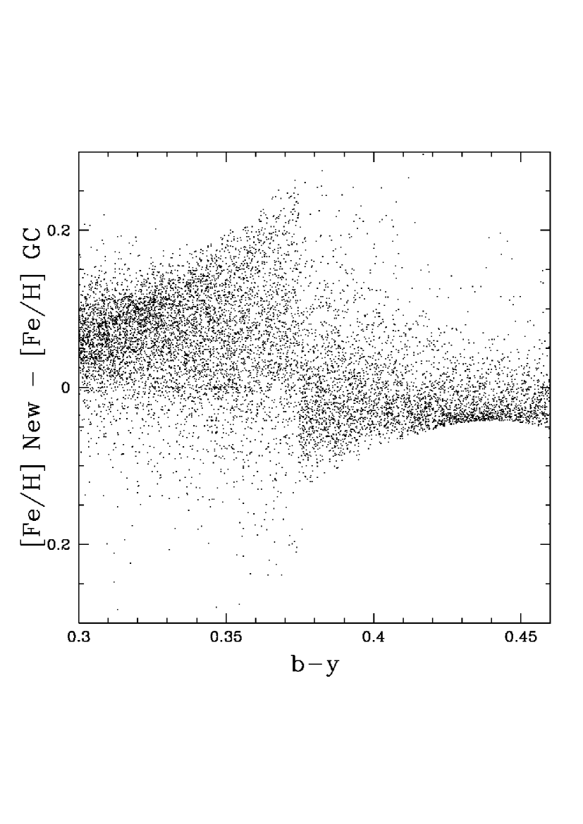
Figure 6: Left: Differences between the GCS metallicities for all stars and those now derived from the GCS blue calibration (the sharp line at $\Delta$[Fe/H]= 0 corresponds to those GCS stars that already used this calibration). Right: The difference between metallicities from the new calibration derived in this paper and the original GCS metallicities, based on the Schuster & Nissen (schuni89 (1989)) calibration.

Fig. 5 compares the photometric [Fe/H] from this calibration with the spectroscopic values; for the stars in common, they again agree very well those from the Schuster & Nissen (schuni89 (1989)) calibration (mean difference 0.02 dex, $\sigma$ only 0.04).

4.2 An improved metallicity calibration

In order to define an improved photometric metallicity calibration that is valid for all GCS stars, we select only spectroscopic investigations using a photometric temperature scale (unlike the compilation of literature values by Cayrel de Strobel et al. (cayrel01 (2001)) used by H06). This yields a total sample of 573 stars from Edvardsson et al. (edv93 (1993)), Chen et al. chenyq00 (2000), Reddy et al. reddy03 (2003), Allende Prieto et al. (allende04 (2004)), and Feltzing & Gustafsson (feltz98 (1998)). They all have a very consistent metallicity scale: Comparing stars in common yields differences of of 0.02 dex or smaller in the mean, with a dispersion of $\sim$0.07 dex. The 573 stars span the range 0.24 $\leq b-y\leq$ 0.63, 0.10 $\leq m_{1}\leq$ 0.70, 0.17 $\leq c_{1}\leq$ 0.53, and -1.0$\leq[\rm Fe/H]\leq$ 0.37.

A new fit of the uvby indices to the spectroscopic [Fe/H] values from this sample was performed, using a calibration equation containing all possible combinations of $b-y,m_{1}$, and $c_{1}$ to third order.

The resulting calibration equation is:

${\rm[Fe/H]}=-2.19-1.02(b-y)+7.34m_{1}-0.27c_{1}\\ +5.86(b-y)^{2}-43.74m_{1}^{2}-0.14c_{1}^{2}+25.03(b-y)m_{1}\\ +5.29(b-y)c_{1}+25.95m_{1}c_{1}-31.10(b-y)^{3}+46.19m_{1}^{3}\\ -3.86c_{1}^{3}+4.54(b-y)^{2}m_{1}+19.31(b-y)^{2}c_{1}-17.46m_{1}^{2}(b-y)\\ +18.36m_{1}^{2}c_{1}-9.99c_{1}^{2}(b-y)+6.60c_{1}^{2}m_{1}-59.65(b-y)m_{1}c_{1}$

This new calibration is used for all stars with 0.30 $<$ b-y $<$ 0.46. Together with the blue and red calibrations already derived in the GCS, this completes the final metallicity calibration of the present paper. All results discussed in the following are based on it.

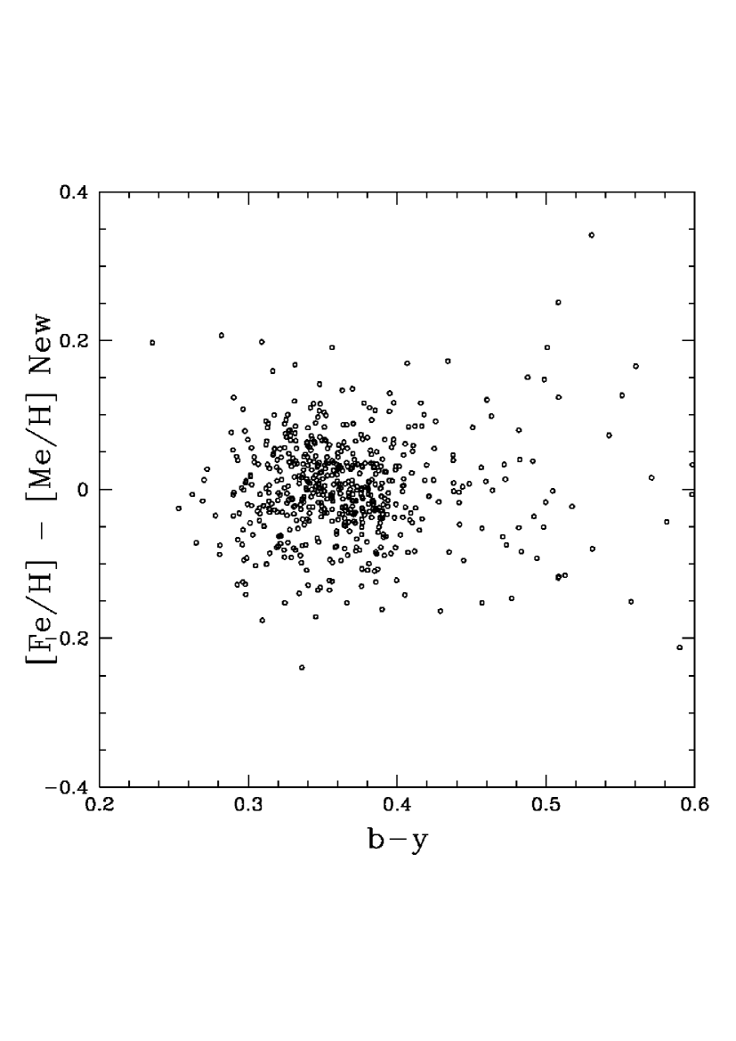
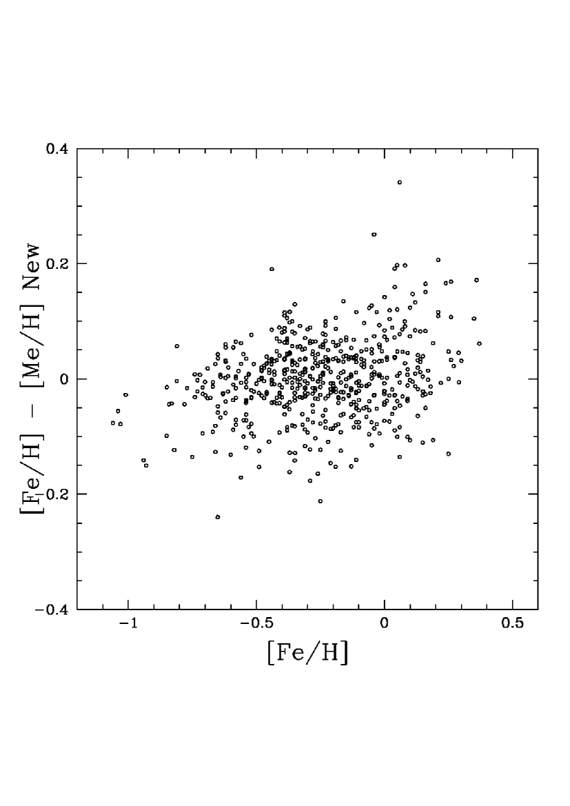
Figure 7: Same as Fig. 4, but using the new metallicity calibration derived in this paper.

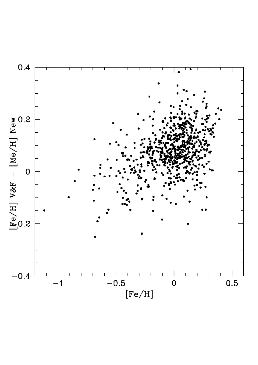
Figure 8: Spectroscopic [Fe/H] data from VF05 vs. our new photometric [Me/H] for the GCS stars.

Fig. 6 shows the differences between the GCS [Fe/H] values and those derived with the new calibration; note that, in the left panel of Fig. 6, the heavy sequence at zero difference is formed by the stars that already then used the blue calibration.

The consistency of the photometric metallicities from this calibration with the spectroscopic reference values is shown in Fig. 7. The dispersion around the mean is 0.07 dex – the same as between two different spectroscopic measurements. The calibration derived above is also in good accordance with the two relations derived in the GCS. Compared to the blue relation, the mean difference is 0.02 (dispersion 0.04) in the common range 0.3$<$b-y$<$0.32. Compared to the red relation, the mean difference is 0.00 (dispersion 0.09) in the common range 0.44$<$b-y$<$0.50.

Finally, Fig. 8 compares our new GCS metallicities with the spectroscopic [Fe/H] values from VF05. The mean difference VF05-GCS is 0.08 dex, with a standard deviation of 0.10 dex. The higher metallicities derived by VF05 are understandable, given the generally higher temperatures they adopt.

Figure 9: Top left: The GCS metallicity calibration applied to the Crawford & Perry (crawfordPerry (1966)) uvby$\beta$ photometry of the Hyades. Top right: Using the new calibration from this paper instead. Bottom left: The GCS metallicity calibration applied to the Crawford & Barnes (crawfordBarnes (1969)) uvby$\beta$ photometry of the Coma cluster. Bottom right: The Coma stars, using the new calibration.

4.3 The Hyades and Coma clusters

One of the two open clusters included in the GCS, the Hyades, has been used by e.g. H06 to assess the zero-point of the GCS metallicity calibration. A comparison with the original uvby$\beta$ photometry of the Hyades and Coma clusters by Crawford & Perry (crawfordPerry (1966)) and Crawford & Barnes (crawfordBarnes (1969)) shows, however, that the photometry of the cluster stars that was listed in the GCS is not on the same system as the rest of the catalogue, perhaps because they were observed at high air mass from Chile. While unfortunate, this offset means that the Hyades data will give misleading results if applied to the metallicities (and thus ages) of the whole GCS catalogue.

The result of using the photometry from the original sources combined with the earlier GCS calibrations is shown in Fig. 9. For the Hyades, we then find $\rm[Fe/H]=0.10\pm 0.10$; for Coma, $\rm[Fe/H]=-0.02\pm 0.08$ (mean and dispersion). The derived [Fe/H] for the Hyades corresponds well to the standard value, as expected because it is mostly based on the Schuster & Nisssen calibration, which used the Hyades as a main anchor point.

Using the new calibration instead yields $\rm[Fe/H]=0.06\pm 0.07$ for the Hyades and $\rm[Fe/H]=-0.09\pm 0.06$ for Coma. The dispersion among the cluster stars is no larger than in the field star calibration, but there is an offset of about 0.07 dex.

A different photometric [Fe/H] for the Hyades is to be expected, considering the non-standard He/Fe ratio of this cluster (Vandenberg & Clem clem03 (2003)), but Coma has a standard chemical mix, and the mean photometric metallicity is very near the accepted spectroscopic value.

In summary, we conclude that it is inadvisable to use the Hyades for general calibrations of photometric metallicities or comparing metallicity scales. The same is true for the ages, especially for the unevolved solar-type stars for which isochrone ages are bound to be very uncertain by any method.

Finally, we note that the revised data in Table 1 for Hyades and Coma stars are based on the standard photometry and can be used with confidence.

4.4 Solar analogs as a test of the calibrations

Solar analogs offer yet another test of the temperature and metallicity determinations. Such stars can be identified through either photometric or spectroscopic resemblance to the Sun – preferably both. 18 Sco (HD 146233) is one of the best known examples, with b-y= 0.404, M_V= 4.77, as compared to the value b-y= 0.403 for the Sun by Holmberg et al. (holmberg06 (2006)), determined by comparison with a carefully selected sample of stars similar to the Sun.

[Fe/H] for 18 Sco is close to zero with both the old (+0.03) and new (-0.02) metallicity calibrations, whereas $\rm T_{eff}$= 5766K as derived from b-y and the new calibration is much closer to that of the Sun than the GCS value of 5689K, in good agreement with the general trend of Fig. 1.

5 Absolute magnitude/distance calibration

In order to determine an improved absolute magnitude/distance calibration for uvby$\beta$ photometry, we selected a sample of 2451 stars with absolute magnitudes better than 0.10 mag from Hipparcos and no indication of binarity in the GCS. A relation using all combinations of b-y, $m_{1}$ and c₁ up to third order was then fitted to the absolute magnitudes of these stars.

The difference between the calibration data and the fitted relation is shown in Fig. 10. The dispersion of the fit is 0.24 mag, but there is a clear excess of stars with large differences, probably due to still-undetected binaries. Repeating the fit after removing stars more than 2.5 $\sigma$ from the mean relation reduces the dispersion to 0.16 mag. The stars span the range: 0.20 $\leq b-y\leq$ 0.60, 0.09 $\leq m_{1}\leq$ 0.64, 0.16 $\leq c_{1}\leq$ 0.80, and -0.84 $\leq{\rm M_{V}}\leq$ 7.24.

The resulting calibration equation, valid within the above parameter ranges, is:

${\rm M_{V}}=2.99+2.68(b-y)+10.08m_{1}+3.14c_{1}+15.27(b-y)^{2}\\ -17.73m_{1}^{2}+26.28c_{1}^{2}-12.73(b-y)m_{1}-20.79(b-y)c_{1}\\ -38.86m_{1}c_{1}-17.47(b-y)^{3}-24.14m_{1}^{3}-8.16c_{1}^{3}\\ -56.98(b-y)^{2}m_{1}+27.86(b-y)^{2}c_{1}+103.32m_{1}^{2}(b-y)\\ -161.55m_{1}^{2}c_{1}-131.37c_{1}^{2}(b-y)+29.51c_{1}^{2}m_{1}\\ +257.37(b-y)m_{1}c_{1}$

${\sigma(\rm M_{V}})$ corresponds to distance errors of only 11% and 7% (with and without 2.5-$\sigma$ outliers). Note that this is the total dispersion, including also the error in the Hipparcos distances. A further check of the new calibration based on the wide physical binaries in the sample confirms this estimate (see Sect. 7.2).

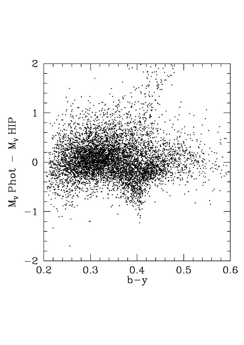
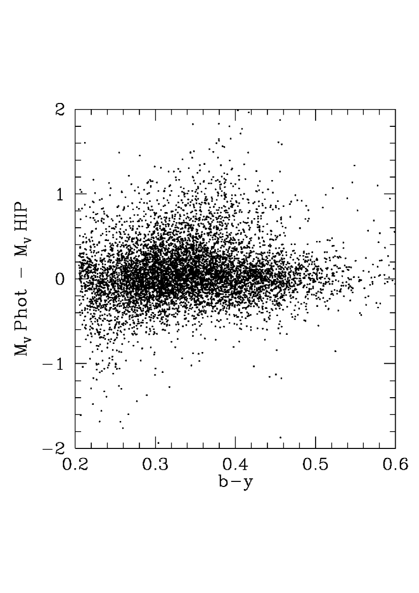
Figure 10: Differences in M_V as determined from uvby$\beta$ photometry and from Hipparcos distances. Left: Original GCS photometric M_V. Right: M_V from our improved calibration.

This relation is a clear improvement over the photometric distance calibration used in the GCS, which had an uncertainty of 13% (0.28 mag). It can also be used to identify further binaries in the GCS catalogue, which only flagged stars with a difference between the Hipparcos and photometric M_V larger than 3 $\sigma$, i.e. larger than 0.84 mag from the photometry alone. We have not, however, recomputed the statistics on binaries in the GCS, as other sources of uncertainty remain important.

As already expected from Fig. 10 in the GCS, there is no systematic difference between the GCS distances and those computed with the above formula (see Fig. 10). However, the uncertainty of the individual distances - which dominates that of the space motions - is reduced enough that we have recomputed the distances and UVW velocity components for all the GCS stars, correcting a minor error in the GCS space velocities at the same time.

6 Interstellar reddening

In the GCS, interstellar reddenings were derived from the intrinsic colour calibration by Olsen (eho88 (1988)), which yields reddening estimates with a stated precision of 0.009 mag. In the GCS there are 827 stars within 40 pc which have E(b-y) estimates. Fig. 11 (left) shows the histogram of these E(b-y) values; a best-fit pure Gaussian shows only a slight zero-point shift of 0.0025 and a dispersion of 0.0105 mag.

Figure 11: Distribution of E(b-y) values from the GCS. Left: Stars within 40 pc (solid) and a Gaussian fit (dashed) for a mean reddening of 0.0025 mag and dispersion 0.0105 mag. Right: Stars with distances 40 – 70 pc and the same Gaussian, showing a significant excess of slightly reddened stars.

The distribution is quite symmetric, showing that it is dominated by observational errors and that real reddening within 40 pc is negligible. This is no longer true for the distance range from 40 to 70 pc, where the distribution is markedly skewed, with a clear excess of true positive extinctions (see Fig. 11, right). Thus, contrary to the assertion by H06, this distance range contains a clear excess of stars with significant positive reddenings; the mean reddening is 0.0048 mag for this sample.

We conclude that the intrinsic colour calibration by Olsen (eho88 (1988)) remains valid with sufficient accuracy for the GCS sample, so we do not recompute E(b-y) and (b-y)₀.

7 Stellar ages

7.1 Review of stellar models

Figure 12: Solar-metallicity 8-Gyr isochrones in the $\rm\log T_{eff}-M_{V}$ diagram. Thick lines: Padova (full); Victoria-Regina (dashed); Yale-Yonsei (dotted). Thin lines: Geneva models: basic (dashed) and “best” low-mass (dotted).

The determination of ages for individual field stars in the range 1-10 Gyr is a field with rich opportunities for large systematic as well as random errors. Some of these arise from the calibrations of the observational data, as reviewed in the preceding chapters. Others are due to the various approximations used in stellar model calculations, especially as regards the treatment of convective core overshooting in this regime of small to vanishing convective cores, and of the stellar atmospheres that are used to compute the observable properties of a model, notably log $g$ and $\rm T_{eff}$.

The density and sampling of the grid of models and/or isochrones are also important in this range, where a major change in isochrone morphology near the turnoff occurs for ages of several Gyr. Other errors again may result from the techniques used to interpolate in the published isochrones and compute masses, ages, and error estimates from the observed data.

In the GCS, great effort was devoted to the derivation of ages and masses and their uncertainties for the stars of the survey, using the sophisticated interpolation method and Bayesian computational techniques of Jørgensen & Lindegren (jorgensen05 (2005)) and accounting for the average $\alpha$-element enhancement of metal-poor stars. Exactly the same method was adopted in the very recent paper by Takeda et al. (takeda (2007)). The theoretical isochrones used in the GCS computations were the latest set from the Padova group (Girardi et al. girardi (2000), Salasnich et al. Salasnich (2000)), while Takeda et al. (takeda (2007)) computed an extensive set of new tracks using the Yale-Yonsei stellar evolution code (Demarque et al. demarque (2004)).

In order to assess the effect of different model prescriptions, we have compared the Padova isochrones to both the Yale-Yonsei (Demarque et al. demarque (2004)) and Victoria-Regina models (VandenBerg et al. vandenberg (2006)) as well as to two different Geneva model series (the “basic” and “best low-mass” models, Lejeune & Schaerer lejeune01 (2001)).

Fig. 12 shows that the differences between the various models are in fact quite small. The difference in age for a star located on the three isochrones in the middle, if derived instead from the two outlying ones, is below 1 Gyr at the turnoff and about 2 Gyr at $\rm M_{V}$= 5, respectively. For the 5 Gyr isochrones, the difference is about 1 Gyr at both points; the larger percentage age spread at the turnoff is related to the slightly different treatment of convective overshooting in the different models. The situation is similar at e.g. [Fe/H]= –0.71, the differences between the isochrones being even somewhat smaller.

Accordingly, in the following we use the same Padova isochrones and $\alpha$-enhancement corrections as in the GCS itself and do not repeat the full age computations with all the different sets of models. This will highlight the effect of changing the calibrations as discussed above, while comparing with the ages computed by VF05 and Takeda et al. (takeda (2007)) will illustrate the effects of photometric vs. spectroscopic input parameter determinations.

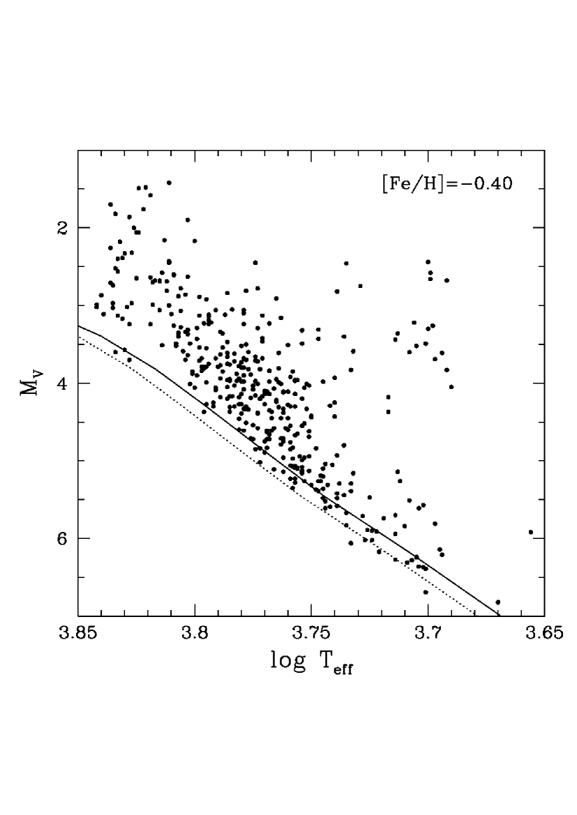
Figure 13: Comparison between the observed single GCS stars with [Fe/H]= +0.23$\pm$0.05, -0.40$\pm$0.05, -0.71$\pm$0.20, and -1.31 $\pm$0.30, after allowing for $\alpha$-enhancement, and ZAMS Padova isochrones with (solid) and without (dotted) temperature corrections.

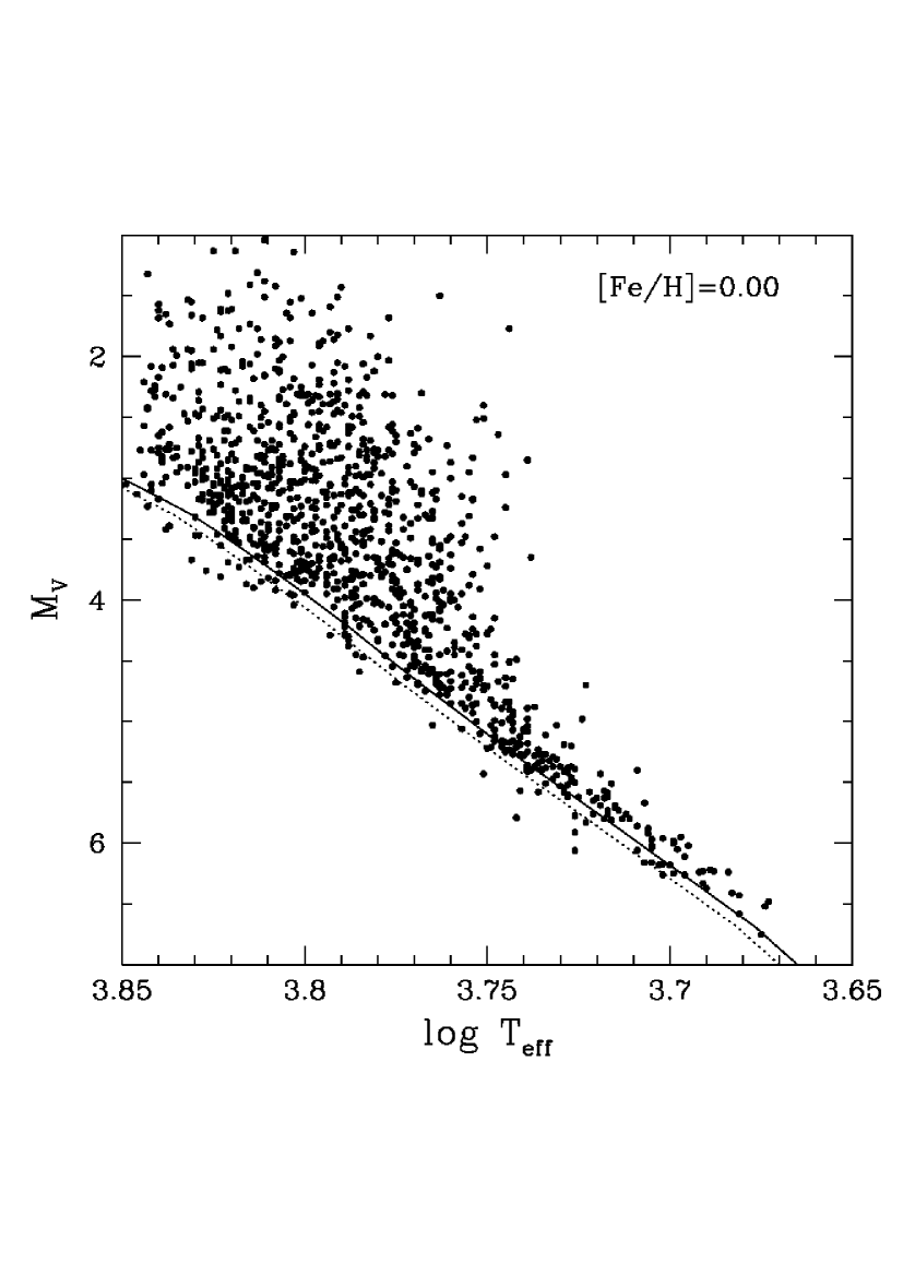
Figure 14: Left: The observed single GCS stars with [Fe/H]= 0.00 $\pm$ 0.03 and the model ZAMS with the new temperature corrections (solid) and without (dotted). Right: Same, for the simulated catalogue (see Sect. 8.1 and Fig. 20 on the sample differences).

7.1.1 The model temperature scale

In the GCS, close attention was paid to verifying the consistency between the computed lower main sequences and the observed unevolved stars. An appreciable offset was found, and substantial, metallicity-dependent, negative temperature corrections were applied to the Padova models to avoid deriving spuriously large ages for the low-mass stars. No similar offset seems to have been found necessary by Takeda et al. (takeda (2007)), perhaps because the Yale-Yonsei models (Demarque et al. demarque (2004)) themselves appear to be somewhat cooler than the Padova models (see Fig. 12). The offset is also masked by the hotter temperatures and higher metallicities they adopt for their stars.

With the new temperature and metallicity calibrations derived in this paper, the temperature corrections applied to the Padova isochrones in the GCS also need revision. We find corrections of $\rm\delta\log T_{eff}$ = -0.005 for [Fe/H] $\geq$ 0, -0.01 at [Fe/H]= -0.40, -0.02 at [Fe/H]= -0.70, and -0.025 at [Fe/H] $\leq$ -1.30 to be needed for the models to match the observed ZAMS; see Figs. 14 and 13.

As a further check, Fig. 14 compares the temperature-corrected solar-metallicity model main sequences with the distribution of stars in the observed catalogue as well as in a simulated sample (see Sect. 8.1) with errors in $\rm\log T_{eff}$, [Fe/H], and $\rm M_{V}$ as observed, both in the range [Fe/H]= 0.00$\pm$0.03. Note that the main purpose of the figure is to illustrate the scatter of stars around the ZAMS due to measurement errors; the model has not been designed to account for the effect of the age-dependent sample volume of the GCS on the distribution of stars in the HR diagram (cf. Sect. 8.1).

Another way to check the temperature corrections is to consider active stars with low chromospheric ages. Fig. 15 compares stars with -0.1$<$[Fe/H]$<$0.1 and chromospheric ages below 1 Gyr from the catalogue of Wright et al. (wright (2004)) to a solar-metallicity 1-Gyr isochrone, corrected as above. As seen, the agreement is again quite satisfactory.

Figure 15: GCS stars with chromospheric ages below 1 Gyr and $\rm-0.1<[Fe/H]<0.1$, compared to a corrected 1-Gyr solar-metallicity isochrone.

Finally, a test can be made using single Hyades stars with photometry from Crawford & Perry (1966). Fig. 16 compares these stars to a 0.7-Gyr corrected isochrone and shows the estimated ages and their uncertainties. The scale offset in the ages is due to the use of a standard Y/Z ratio in the models, which is incorrect for the Hyades (Vandenberg & Clem clem03 (2003)).

Figure 16: Left: Single Hyades stars compared to a corrected 0.7-Gyr isochrone for [Fe/H]= +0.15. Middle: Estimated ages and uncertainties; the scale offset is due to the non-standard Y/Z ratio of the Hyades. Right: Age-metallicity relation for the Hyades computed as for the whole catalogue, including only stars with age errors below 25%.

7.2 Consistency checks with wide binaries

Wide physical binaries as confirmed by proper motions and radial velocities provide another check of the accuracy of our metallicity, distance, and age determinations. We have selected 18 such pairs from the GCS, with separate measurements of all parameters and no indication of further multiplicity. The pairs have a wide distribution in [Fe/H], from -0.4 to +0.1, and ages in the range 0–10 Gyr. Fig. 17 shows a typical example.

With the GCS calibrations, the rms difference in [Fe/H] between the two components is 0.11dex; using the new calibrations reduces it to 0.06 dex, in excellent agreement with our other error estimates. Similarly, using the new photometric distance calibration (Sect. 5) instead of the older ones used in the GCS reduces the average difference in distance between the binary components from 16$\pm$3% to 12$\pm$3% (s.e. of mean).

The accuracy of the age determination can be estimated from the ratio of the age difference between the two binary components, $\Delta Age$, and the combined 1$\sigma$ uncertainty of the two ages, $\sigma Age$. For the GCS ages we find $<\Delta Age$/$\sigma Age>$= 0.87. Recomputing the ages and age uncertainties for the binary components, using the new calibrations and (lower) estimated errors for [Fe/H], $\rm T_{eff}$ from b-y, and photometric $\rm M_{V}$ as well as the newly corrected isochrones, we find $<\Delta Age$/$\sigma Age>$= 0.76. In other words, the age estimates become more consistent as well as more precise with the new calibrations.

Figure 17: ${\rm M_{V}}$, [Fe/H], and ages for the components of the physical pair HD 130140/1. The isochrone shown is for the best mean age of 9 Gyr. $\Delta Age$/$\sigma Age$= 0.74 for this pair.

7.3 New ages vs. the GCS ages

Fig. 18 compares the GCS ages, computed with the old [Fe/H] and $\rm T_{eff}$ calibrations, with the ages computed using the new calibrations and model corrections from this paper. Overall, the differences are insignificant, much smaller than the estimated individual uncertainties. A linear fit gives the following mean relation between the new ages and those in the GCS: $\rm Age_{New}=0.16+0.90\times Age_{GCS}$ (all ages in Gyr). Thus, on average, the largest ages decrease by $\sim$10%. This is similar to the differences seen when using different stellar models and has negligible impact on the interpretation.

Figure 18: Ages based on the new metallicity and temperature calibrations and model corrections vs. the original ages GCS, using only single stars with ages better than 25% in both sets. The dotted line shows the 1:1 relation.

The only noteworthy deviations occur on the two “branches” that can be seen in Fig. 18. This small group of stars is located in the “hook” region in the HR diagram, where an observed point is matched by two different isochrones, one placing the star on the main-sequence turnoff, the other on the early subgiant branch. As explained e.g. in Jørgensen & Lindegren (jorgensen05 (2005)), this leads to a two-peaked G-function structure. Small changes in the assumed [Fe/H] and $\rm T_{eff}$ may then change the relative height of the peaks, and thus the most probable age of the star. For such double-peaked G-functions, one could use a weighted mean of the two maximum values rather than a simple fit to the highest peak, but the improvement would be cosmetic rather than real.

Table 1: Sample listing of the recomputed parameters for the first five stars in the GCS catalogue. $Age_{low}$ and $Age_{up}$ are the lower and upper 1-$\sigma$ confidence limits on the computed age, respectively. The full table is available in electronic form from the CDS (see reference on title page).

HIP	Name	Comp	RA ICRF	Dec ICRF	$\rm logT_{e}$	[Fe/H]	d	$M_{v}$	Age	$Age_{low}$	$Age_{up}$	U	V	W
			h  m   s	o   ′  ′′			pc	mag	Gy	Gy	Gy	km s-1	km s-1	km s-1
1	2	3	4	5	6	7	8	9	10	11	12	13	14	15
437	HD 15		00 05 17.8	+48 28 37
431	HD 16		00 05 12.4	+36 18 13
420	HD 23		00 05 07.4	–52 09 06	3.776	-0.17	42	4.44	3.7	0.3	6.3	40	-22	-16
425	HD 24		00 05 09.7	–62 50 42	3.768	-0.33	70	3.91	8.5	7.5	9.6	-31	7	14
	HD 25		00 05 22.3	+49 46 11	3.824	-0.30	79	3.09	2.0	1.8	2.2	17	0	-22

Finally, we compare our results to two recent sets of ages, both computed from the spectroscopic results by VF05. One set is given in that paper itself, using a relatively crude method, while the more recent one by Takeda et al. (takeda (2007)) was computed with the same Bayesian technique as used in the GCS, based on a dense grid of stellar evolution tracks computed with the Yale-Yonsei code (Demarque et al. demarque (2004)). In order to avoid confusion by including stars with highly uncertain ages (see, e.g. Fig. 8 of Reid et al. reid07 (2007)), we select only single stars with ages better than 25% as given by both sources.

Figure 19: Left: New ages vs. ages from VF05. The sample consists of single GCS stars with both new and VF05 ages better than 25%; the 1:1 relation is shown. Right: The same comparison with ages from Takeda et al. (takeda (2007)).

Fig. 19 shows the remarkable result of this comparison. While the VF05 ages are on average $\sim$10% lower than ours, those by Takeda et al. (takeda (2007)) are in essentially perfect agreement with ours. Considering that these results are based on totally different observational data and analysis techniques, calibrations, and stellar models, the agreement is extraordinarily close and inspires a solid confidence in age determinations from isochrones. Note that the differences between Takeda et al. (takeda (2007)) and VF05 are due to different computational techniques applied to the same data, while the differences between the old and new GCS ages are due to improved calibrations, the computational method remaining the same. That the systematic differences seen in both cases are only of the order of $\sim$10% gives further confidence in the robustness of the method.

For future reference we recall that, temperature and metallicity calibrations aside, the age estimates computed by H06 were based on an unrealistically small value for the uncertainty of $\rm T_{eff}$. Further, the computations ignored the uncertainty in $M_{V}$ as well as the temperature offset of the models, the $\alpha$-enhancement of the metal-poor stars, and the presence of binaries in the sample. Moreover, the bright limit of $M_{V}$=2 excluded many young stars for which good ages can be readily determined (see GCS Fig. 11a), while at the same time including low-mass giants for which meaningful ages cannot be derived. Finally, the uncertainty of the resulting ages was not discussed.

8 Results and sample characteristics

Based on the new calibrations and model corrections discussed above, we have computed new $\rm T_{eff}$, [Fe/H], distances, ages and age uncertainties, and space motions for all the stars in the GCS. Table 1 gives the results; the full version is available in electronic form at the CDS. We have not recomputed Galactic orbital elements for the stars, as uncertainties in the assumed (smooth, axisymmetric) potential are more important than minor revisions of the space motions. In the following, we discuss the implications of the new data for our understanding of the evolution of the Milky Way disk.

In such discussions, it is crucial to not only employ the best possible calibrations from observed to astrophysical parameters, but also to understand to what extent the criteria used to select the stellar sample may influence the conclusions drawn. This is especially important when studying subsamples selected on the basis of having one or more of the derived parameters available, perhaps within a certain level of precision, rather than the entire GCS. Age is the most striking example: The samples of stars having ages better than 25%, or “well-defined” ages in the GCS sense, or any ages at all, are all very different from the full GCS sample in very non-random and non-intuitive ways.

Much effort was spent checking these issues in preparation for the GCS. Only overall results were mentioned in the paper itself, details being left to the present paper. These tests are the subject of the following sections.

8.1 Simulating the sample selection effects

To estimate the interplay between the sample selection criteria and any errors in the determination of the derived parameters in the GCS, we have performed an extensive set of numerical simulations based on a synthetic catalogue. The synthetic catalogue assumes a constant density of stars in a spherical volume of $\sim$250 pc radius, a mixture of 90% thin-disk and 10% thick-disk stars with an even distribution in stellar age and evolutionary stage. Several distributions in metallicity and kinematics were imposed on the thin disk in order to explore the possible systematic effects; for the thick disk we assumed an asymmetric drift in $V$ of 65 km s${-1}$ and ($\sigma_{U}$,$\sigma_{V}$,$\sigma_{W}$) = (72,43,36) km s^-1.

The star density was normalised such that, after applying the appropriate cutoffs, the resulting sample would contain about 15 000 stars total, with about 97% thin-disk and 3% thick-disk stars, as observed. Each component has a distribution in metallicity and kinematics similar to the observed values, and the distribution of stellar parameters and measurement errors is also like the real catalogue. In order to better test the age estimation process at faster evolutionary stages, the stars are more uniformly distributed along the isochrones than what would result from a standard IMF.

By applying the various calibrations, computations, and parameter cuts to the simulated catalogue in parallel with the observed sample, we can ascertain in quantitative terms which systematic effects may be introduced at each stage and whether they have any significant influence on the conclusions.

Figure 20: Average volume occupied by single stars with “well-determined” ages in the real GCS (full line) and in the simulated catalogue with a fixed apparent magnitude limit of $V$= 8 (dotted).

As a first example, we show how the volume of space sampled by the GCS varies with age. Because older stars are, on average, fainter (and cooler) than younger stars, and the GCS sample is limited by apparent magnitude, the volume sampled by the GCS decreases with stellar age. GCS Fig. 24 showed this effect as a function of colour; here we illustrate the dependence on age directly by imposing a simple apparent-magnitude cutoff at $V$= 8 and computing the average volume occupied by the stars in successive 1-Gyr age bins, normalised to that occupied by the youngest stars (=100%).

Fig. 20 compares the result for the simulated sample (dotted curve) with the same computation for the real GCS (full line). Only single stars with “well-determined” ages are included. The GCS adopts fainter limiting magnitudes for the redder stars in order to achieve volume completeness to 40 pc, so the fraction of older stars is higher than for the simplified simulation.

However, the origin of the preponderance of young stars in, e.g., Figs. 23 and 29 is clear: They are included from a volume $\sim$5 times larger than the stars older than $\sim$3 Gyr. Accounting properly for these sampling volume differences is, of course, crucial when deriving the star formation history of the solar neighbourhood from the data – a study we do not undertake here.

More specific simulations have been carried out to test the most significant conclusions of the GCS; they are described in the following as appropriate in each context.

9 The metallicity distribution function

Models of star formation and chemical evolution in the galactic disk make predictions of the distribution of heavy-element abundances in stars that (could) have survived from all stages of the evolution. The classic failure of ’closed-box’ models – the so-called “G-dwarf problem – refers to the observed lack of those metal-poor dwarf stars that should have accompanied the high-mass stars that produced the heavy elements we do observe in the younger stars, assuming a constant IMF. One may ask whether the metallicity calibration or the way the data are compared with the models may cause a spurious difference.

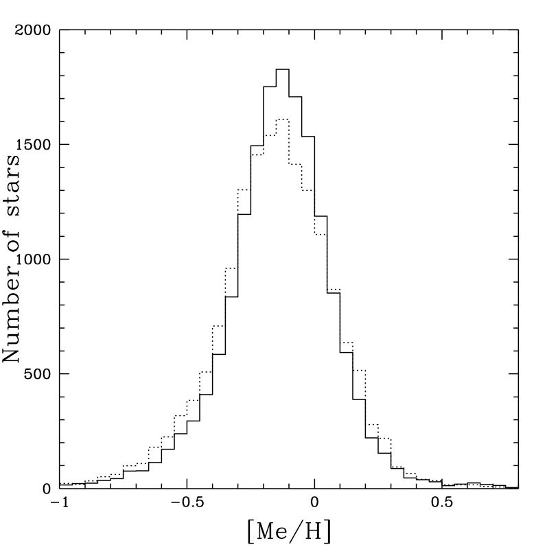
Figure 21: Left: Metallicity distribution function for all stars using the new calibration (solid) as well as the original GCS values (dotted). Right: The distribution of $\rm T_{eff}$ with the new and old calibrations (same symbols).

Fig. 21 compares the distributions of the GCS stars in [Fe/H] and $\rm T_{eff}$ as derived with the old and new calibrations. As seen, the new calibration leads to even fewer metal-poor stars in the sample than the old one, but the difference is marginal.

Galactic evolution models typically predict average properties of the stellar population in a vertical column through the disk at the position of the Sun, while observations typically – as in the GCS – refer to a roughly spherical volume centred on the Sun. Knowing the motions of the stars enables us to allow for this difference.

Figure 22: Left: The $W$ velocity dispersion as a function of [Fe/H] for the volume-complete sample (equal-size bins). Right: Metallicity distribution function for stars in the volume-complete sample (solid); in the column, using the fit in the left-hand panel (dashed); and in the closed-box model of Casuso & Beckman (casuso04 (2004), thin line).

We have performed the correction from a volume-complete to a column-complete sample in a rigorous manner, using the self-consistent mass models of the disk derived by Holmberg & Flynn (holmberg00 (2000), holmberg04 (2004); latest version in Flynn et al. holmberg06 (2006)). With this model, we derive the relation between volume and column density for each velocity dispersion. Fig. 22 shows the vertical velocity dispersion of the GCS stars as a function of metallicity, together with a smooth polynomial fit. This fit is then used to transform the volume densities to corresponding column densities as functions of [Fe/H].

Fig. 22 compares the volume and column metallicity distribution functions with each other and with a closed-box model without instantaneous recycling approximation (Casuso & Beckman casuso04 (2004)), convolved with a Gaussian of $\sigma$= 0.08 to account for the observational error in [Fe/H]. Clearly, neither the calibration nor the volume/column correction can account for the observed dramatic deficiency of metal-poor stars relative to the model.

We cannot comment on the reasons why H06 reached a different conclusion from the same data (albeit with a different metallicity calibration), since the closed-box model discussed by H06 was not described there.

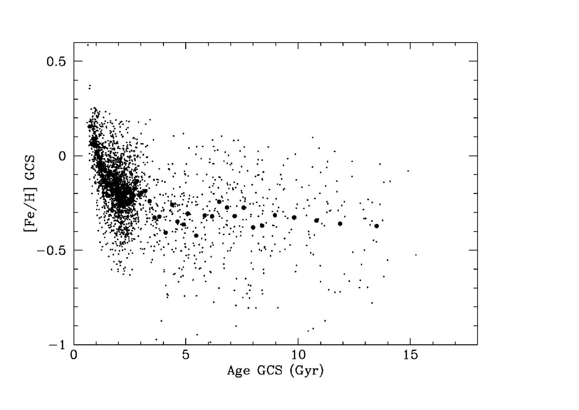
Figure 23: Top: AMR from the original GCS, for single stars with ages better than 25% and with E(b-y) $<$ 0.02 or $d<$ 40 pc. Large dots are mean values in bins with equal numbers of stars. Bottom: Same, using the improved stellar parameters.

Figure 24: Same as Fig. 23, but only for the volume-limited sample with $d<$ 40 pc.

10 The age-metallicity diagram

The relationship between average age and metallicity for stars in the solar neighbourhood – the so-called age-metallicity relation (AMR) – is probably the most popular diagnostic diagram for comparing galactic evolution models with the real Milky May. There is, however, no consensus on its shape or interpretation.

The discussion centres essentially on (i) the presence or absence of a general slope of the AMR (a gradual increase in mean [Fe/H] with time), and (ii) how much of the scatter in [Fe/H] at any given age is accounted for by observational errors and how much reflects the complexity in the evolution of a real galaxy as compared to most current models. It is thus crucial to ascertain whether the distribution of stars in the age-metallicity diagram (AMD) reflects primarily the intrinsic properties of the sample or primarily artefacts of the measurement and parameter calculation procedures.

This can be investigated by means of our simulated sample. First, we check whether the new calibrations have by themselves caused any significant change in the AMD, using the stars with the very best ages ($\sigma(Age)<$25%). In order to eliminate the bright, distant early F stars in the GCS whose high [Fe/H] we suspected to be due to overestimated reddening corrections, we have limited the sample to single stars within 40 pc or with E(b-y) $<$ 0.02 mag. As seen, the revised calibrations cause hardly any difference in the AMD, neither for the full sample (Fig. 23) nor for the strictly volume-limited one (Fig. 24).

Perhaps the most obvious structure in the observed AMD is the marked increase in mean metallicity and the absence of metal-poor stars for ages below 2 Gyr (see Fig. 23 and GCS Figs. 27-28). It is important to understand if this is due, at least in part, to the selection criteria used to define the catalogue sample, or whether it is a genuine property of the solar neighbourhood. In the latter case, it could be interpreted as a cut-off in the resupply of fresh low-metallicity gas, followed by closed-box evolution.

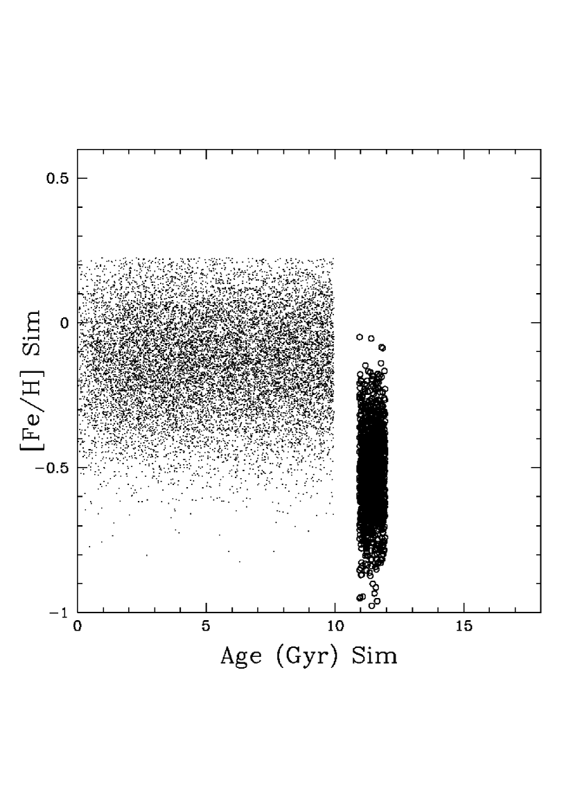
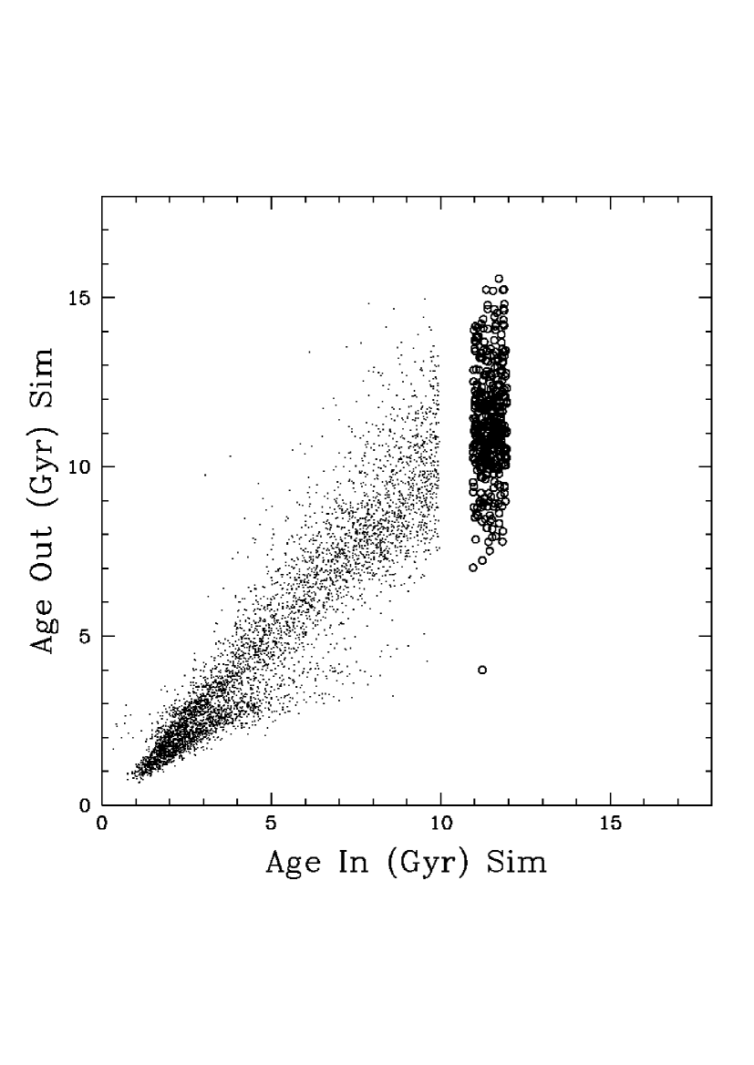
Figure 25: AMR simulations for the synthetic sample. Top left: Input AMR for a volume complete synthetic sample, flat within each of the thin and thick disks (dots and open circles, respectively). Top right: “Observed” AMD for the synthetic sample, using the new calibrations with the synthetic observations and retaining only stars with resulting ages better than 25%. Bottom left: “Observed” AMD as above, but after imposing a blue colour cutoff (b-y $\geq$ 0.205) and apparent magnitude limit as in the GCS. Bottom right: Derived ages vs. the “true” input values.

Fig. 25 shows the results of computing the “observed” AMR from a simulated sample with a flat input AMR (first panel). The second panel shows the effect of recomputing the ages and metallicities from the synthetic data, using the new calibrations and restricting the sample to stars with ages better than 25%. This illustrates the varying difficulty of determining precise ages over the HR diagram, especially in the region where isochrones overlap at 4-5 Gyrs.

The third panel shows the AMR after applying the same blue colour cutoff (b-y $\geq$ 0.205) and apparent magnitude limit as used to define the GCS sample. It exhibits the same preponderance of young metal-rich stars as the observed diagrams (Figs. 23 - 24). Thus, the apparent lack of young metal-poor stars in the AMD is caused simply by the blue colour cutoff of the GCS. None of these selection effects seems to have been considered by H06 or by Reid et al. (reid07 (2007)).

In order to verify whether our calibrations or age computations could introduce (or remove) trends at higher ages in the AMD, we imposed tight AMRs (width 0.1 dex at all ages) on a subset of the simulated catalogue. In order to test all combinations of age and metallicity, we imposed both a linear increase as well as a linear decrease of [Fe/H] with time. We then computed synthetic colours for the stars with random errors as observed, and processed these synthetic stars with the new calibrations in the same manner as in the GCS, including the colour cutoffs, and retaining only stars with ages better than 25%.

Figure 26: Alternative input and “observed” AMRs for the synthetic catalogue (Fig. 25 showing a flat AMR). Left: Input AMR: A 0.10 dex wide band of slope -0.036 dex/Gyr. Right: Same, but with the opposite slope (+0.036 dex/Gyr).

Fig. 26 compares the input and recovered AMD for both of these cases. As can be seen, the slope of the input AMR is faithfully reproduced in both cases, despite the inevitable scatter introduced by the observational errors. We thus conclude that the absence of a significant mean slope of the data points in Fig. 24 reflects the true situation of the solar neighbourhood.

Focusing on the stars older than 4 Gyr in Fig. 24, we find a mean [Fe/H]= -0.24 dex and standard deviation $\sigma$= 0.22 dex for the original GCS data (top panel, 70 stars), and a mean [Fe/H]= -0.21 dex and $\sigma$= 0.21 dex using the new calibrations (bottom panel, 75 stars). Subtracting the estimated observational error in each case (0.10 and 0.07 dex) yields an intrinsic (“cosmic”) scatter in [Fe/H] at a given age of 0.20 dex – identical to the result by Edvardsson et al. (edv93 (1993)) from high-resolution spectroscopy.

We conclude the discussion by reiterating the importance of the sample selection on the resulting AMR. If certain types of stars are excluded a priori, the gross shape of the AMR may be predetermined whatever new metallicities or ages may be observed. Fig. 27 illustrates this, using two popular sources, VF05 and Edvardsson et al. (edv93 (1993)). Both were selected for specific purposes, and both are prone to selection effects affecting the AMR.

Figure 27: AMR for two pre-selected samples using different metallicity and age determination methods. All ages have errors below 25%. Top left: The VF05 sample, using our data. Top right: The Edvardsson et al. sample, using our data. Bottom left: The VF05 sample, using their data. Bottom right: Same, using Takeda et al. ages.

Edvardsson et al. selected evolved F-type dwarfs in order to be able to determine isochrone ages, excluding a priori any old, metal-rich and therefore redder (i.e. G) stars that might have populated the upper right-hand part of the AMR. VF05 studied stars used in planet searches and thusavoided stars with weak lines, i.e. hot metal-poor stars in the opposite corner of the AMR. These facts are clearly discussed in the papers, but make these and other inherently biased samples unsuitable for discussions of the general AMR of the solar neighbourhood.

10.1 AMR slope vs. a radial metallicity gradient

Recently, Rocha-Pinto et al. (rochapinto06 (2006)) interpreted an observed variation of mean metallicity with the difference between the mean orbital radius of the star (R_m) and that of the Sun (R_⊙) as evidence for a tight age-metallicity relation in the thin disk. However, because their values of R_m range from 6 to 9 kpc, many of their stars must have large velocities and orbital eccentricities, usually associated with thick-disk stars. This was already noted by Edvardsson et al. (edv93 (1993)), although they did not use the explicit term “thick disk”.

A much more natural explanation of the apparent radial variation in metallicity is that the observed stellar sample is a mix of thin-disk stars dominating close to the solar circle, and thick-disk stars dominating at both high and especially low R_m. To verify this, we have compared the observed radial metallicity distribution for single stars in the GCS (using the new calibrations) with that of our simulated catalogue, which has the flat age-metallicity distribution of Fig. 25, i.e. no correlation between age and metallicity in either the thin or the thick disk. However, we have added a radial metallicity gradient of -0.09dex/kpc for the thin-disk stars, close to the observed values (see, e.g., discussion in Sect. 6.2 of the GCS). Fig. 28 shows that this reproduces the observed radial metallicity variation without any variation of metallicity with age.

Figure 28: Radial variation in [Fe/H] for the single GCS stars (dots; new calibration), and for a simulated catalogue with the AMD of Fig. 25 (line), i.e. with no correlation between age and metallicity in either the thin or the thick disk, but a radial metallicity gradient of -0.09 dex/kpc in the thin disk. We obtain a similar overall relation as Rocha-Pinto et al. (rochapinto06 (2006)), but without any AMR in either thin or thick disk.

We have deliberately made no attempt to fit the detailed structure in the R_m - [Fe/H] distribution. This depends on the complex structure of the distribution of the U and V velocities (see Figs. 29 - 30 and GCS Fig. 20), which exhibits a multitude of kinematic groups not accounted for in a simple diffusion picture. As an example, the peak in [Fe/H] at R${}_{\rm m}\simeq$ 6.8 kpc is associated with the $\zeta$ Herculis stream discussed in the GCS and again by Famaey et al. (famaey05 (2005)) and Bensby et al. (bensby07 (2007)).

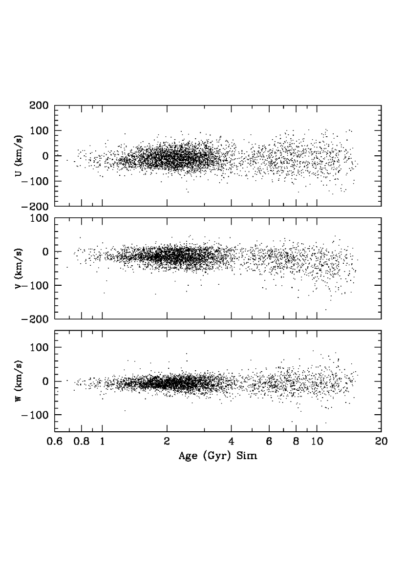
Figure 29: U, V and W velocity vs. age for the 4065 single GCS stars with $\sigma(Age)<25$%).

Figure 30: U-V diagrams for the GCS subsample of Fig. 29, separated into four age groups.

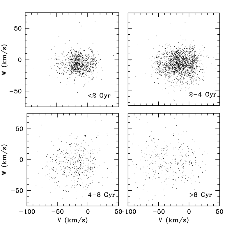
Figure 31: V-W diagrams for the GCS subsample of Fig. 29, separated into four age groups.

Figure 32: W velocity distributions for the GCS subsample of Fig. 29, separated into four age groups. No significant substructure is seen.

11 Age-velocity relation and disk heating

As demonstrated earlier in this paper, our new calibrations cause no significant systematic changes in the velocities and ages of the GCS stars (apart from the overall $\sim$10% age scale reduction). Thus, no major revision of the GCS results on the evolution of the kinematics of the disk with age is to be expected. However, the size of our sample allows us to examine that evolution in greater detail than was done in the GCS.

For this task, we select the cleanest sample of GCS stars, i.e. the single stars with $\sigma(Age)<25$% and with complete space velocity data. Note that, due to our improved age determination, there are now 4065 stars in this class as compared to 2852 in the original GCS – an increase by almost 50%.

Figure 33: Velocity dispersions vs. age for the GCS subsample of Fig. 29 (4065 single stars with $\sigma(Age)<25$%; new calibrations). The 30 bins have equal numbers of stars; the lines show fitted power laws. The 3 youngest and oldest bins have been excluded from the fit.

Fig. 29 shows the observed space velocity components as functions of age, while Figs. 30 and 31 show them in the U-V and V-W planes, separated into four groups by age. Like Figs. 20 and 30 of the GCS, they illustrate the significant substructure in the $U$ and $V$ velocity distributions that persists over a wide range of ages (see also Famaey et al. famaey05 (2005) and the study of the Hercules stream by Bensby et al. bensby07 (2007)). In contrast, the $W$ velocities show no deviation from a random distribution in any age group (Fig. 32), suggesting that different heating mechanisms are at work in the plane of the disk and perpendicular to it. However, it must also be noted that phase mixing is stronger for vertical motions due to the Galactic potential, and the orbital periods shorter, resulting in a more efficient smoothing of structure.

A detailed discussion of the mechanisms affecting disk star orbits in and perpendicular to the plane is beyond the scope of the present paper, but we can consider two basic questions, i.e. (i) whether the velocity dispersion of disk stars continues to increase during the lifetime of the disk or whether it shows signs of a plateau or saturation in some age interval, and (ii) what functional form appears appropriate for the rising parts of the age-velocity relation (AVR). For this discussion, we divide the sample by age into 30 bins with equal numbers of stars (i.e. 135 in each bin), against the only 10 bins used in the GCS; this allows us to follow the evolution in greater detail.

Fig. 33 shows the resulting AVR, which shows a smooth, general increase of the velocity dispersion with time in both U, V, and W. Fitting power laws while excluding the three youngest and three oldest bins, we find exponents of 0.38, 0.38, 0.54 and 0.40 for the U, V, W and total velocity dispersions – slightly larger than the values derived in the GCS, as expected from the change in age scale.

This, however, is clearly not the full story of the phenomenon known as “disk heating”. If that term is taken to refer to an increase in the random motions of disk stars, it is clear from Fig. 30 that the present distribution of the U,V velocities is not the result of pure “heating”; non-random processes are at work as well. Several possible mechanisms have been described in modern literature, based on detailed simulations, but all result in velocity dispersion increases with time that can be approximated by a power law. This is true, e.g. for the simulations that use transient spirals as the heating agent (De Simone, Wu & Tremaine desimone (2004)) or produce velocity structure and heating of the disk by interaction between two spiral systems (Minchev & Quillen minchev (2006)) or between a spiral and the bar (Chakrabarty chakrabarty (2007)).

To identify any underlying “pure” heating mechanism within the disk, one would have to remove the major non-random substructures, such as the Hercules stream or the Sirius UMa, Coma, and Hyades-Pleiades branches (GCS; Famaey et al. famaey05 (2005); Bensby et al. bensby07 (2007)). This, however, introduces a certain arbitrariness as to the choice of stars to be removed; and it appears more interesting to us to identify the cause(s) of the substructures that dominate the U,V plane than to quantify any remaining minor effects.

On the other hand, the observed heating of the vertical (W) velocities, which show no signature of non-random mechanisms, is more efficient than found in simulations. E.g. Hänninen & Flynn (hanninen (2002)) find an exponent of only 0.26 using molecular clouds and need massive black holes to reproduce the observed heating rate, in agreement with several earlier studies. The black-hole hypothesis is inconsistent with other observational data, but the extra vertical heating might be due e.g. to infalling satellites with dark matter substructure (Benson et al. benson (2004)). In any case, further theoretical work on the heating mechanisms affecting the vertical velocities in the disk will have to satisfy the observational constraint illustrated in Fig. 33.

This conclusion contrasts with that by Quillen & Garnett (quillen01 (2001)), who claimed that the heating of thin-disk stars saturates at a maximum velocity dispersion $\sim$3 Gyr after the birth of a star; the oldest stars were assumed to belong to the thick disk and heated by a different mechanism. This led Freeman & Bland-Hawthorn (freeman02 (2002)) to suggest that remnants of early mergers might still be traced as dynamical groups in the disk today (see Helmi et al. helmi06 (2006) for an actual application).

Fig. 33 shows no such saturation in our data, but the levelling-off of the velocity dispersion in the two oldest bins might be taken as weak evidence for a constant velocity dispersion in the thick disk. When judging the merits of the two results, it should be remembered that the sample discussed here is some 20 times larger than that discussed by Quillen & Garnett (quillen01 (2001)) and the sampling errors correspondingly smaller.

Finally, we want to verify whether our age computation techniques might bias the slopes seen in the age-velocity relation (AVR). To do so, we have imposed a fixed AVR on our synthetic catalogue, assuming purely Gaussian velocity distributions and adopting the slopes of $\sigma(U,V,W)$ vs. time as derived above. The thick disk contribution in the simulation is at the same level as in the observed sample, about 3% after applying the apparent-magnitude cutoff. We then recomputed the ages and age errors for all stars in the synthetic sample, using our new calibrations and retaining only stars with (new) ages better than 25%, sorted the stars into 30 equal-size bins, and recomputed the velocity dispersion in each bin.

The input and reconstructed AVRs are compared in Fig. 34. Symbols with error bars show the “observed” points with recomputed ages and age bins. As can be seen, all the reconstructed velocity dispersions are quite consistent with the input AVRs over the range 1.5 – 8 Gyr. There is thus no evidence for any error or bias being imprinted on the AVR from the age estimation process.

Figure 34: Age-velocity relations for the synthetic sample. Solid lines: Adopted input relations for thin-disk stars. Symbols and error bars: Recomputed ages and velocity dispersions in 30 equal-size bins for stars with ages better than 25%. Dotted lines: Fitted power laws.

12 Thick disk vs. thin disk

In the literature, different criteria are used to distinguish thick-disk stars from the more numerous thin-disk stars in the Solar neighbourhood, based on kinematics, detailed chemical composition, or age. There is, however, no real consensus on what limiting values to adopt in any of these parameters, and the allocation of any individual star to either disk component is often ambiguous. Questions of current interest include the fraction of thick-disk stars in the Solar neighbourhood as well as the existence or otherwise of an AMR in the thick disk.

The thick disk of the synthetic sample is well visible in the reconstructed AMR and AVRs, especially among the oldest stars, where it dominates. In order to estimate the fraction of thick-disk stars in the GCS, we calculated the fraction of thick-disk stars in the simulated catalogue with V-velocities below -100 km/s and [Fe/H] $>$ -1. This sample contained 27% of the total number of thick-disk stars in the catalogue, and no thin-disk stars were found in this velocity-metallicity domain. In the real, observed GCS we find 67 stars in this region. Thus, if we assume the same thick-disk velocity distribution as in the simulation, we find a total of 248 thick-stars; as the total number of single stars with complete space velocities in the GCS is 8479, the thick-disk fraction is thus 2.9%.

As regards a possible AMR in the thick disk we note that, interestingly, the “observed” AMR for the simulated thick-disk stars in Fig. 25 shows a pronounced AMR of slope -0.022 dex/Gyr, although the input “true” AMR had a constant metallicity between the assumed thick-disk age limits of 11 and 12 Gyr. This effect would have been even more pronounced if our strict quality criteria on accepted ages had not been applied (as in H06), or if the thick-disk sample had contained a small fraction of stars with younger ages and/or higher metallicity.

Samples of field thick-disk stars can be constructed by combining different membership criteria. For nearby field stars, a kinematic criterion is most commonly used, based on a decomposition of the local velocity distribution into Gaussians corresponding to the thin and thick disk and assuming values for the asymmetric drift and U,V,W velocity dispersions for each. Membership probabilities for either disk are then assigned for each star, based on the observed space motion.

First, as shown in Fig 30 and GCS Fig. 20, the actual local velocity distribution is nothing like a two-Gaussian model; in particular, the $\zeta$ Herculis stream occupies a position near the overlap between the thin and thick disks. Second, Fig. 34 shows that the practice of assuming a single set of velocity dispersions for the thin disk, regardless of age, ignores the effects of the continuing dynamical heating of the disk. As general thin-disk samples are typically dominated by relatively young stars (see Figs. 23 and 29), the mean values of $\sigma(U,V,W)$ will tend to be underestimated, enhancing the probability that thin-disk outliers will be classified as thick-disk stars.

If the thick disk is indeed very old, as is most commonly assumed, the kinematic parameters characterising the thin disk should be chosen to correspond to the oldest thin-disk stars (see Fig. 34). It is interesting to note that Bensby et al. (Bensby04 (2004)), who identify thick-disk stars with intermediate ages and chemical properties, assume significantly lower values of $\sigma(U,V)$ for the thin disk than Reddy et al. (reddy06 (2006)), who find a smaller fraction of such stars and consider them to be outliers from the thin disk.

Given the inherent ambiguity of kinematic population indicators, the enhanced [$\alpha$/Fe] ratio observed in thick-disk stars may be the best membership criterion for individual field stars. In order to study the AMD of the thick disk from the cleanest possible sample of stars, we therefore selected all stars in common between the GCS and those kinematically classified thick-disk stars from Reddy et al. (reddy06 (2006)) that also have $\rm[Ti/Fe]>0.25$.

Fig. 35 shows the AMD for this “clean” thick-disk sample, using our new ages. We see a tight grouping of stars with ages around 11 Gyr and $\rm[Fe/H]\sim$ -0.55, and no trace of a slope. Taken together, Figs. 25 and 35 put into question the claims of a significant age-metallicity relation in the thick disk by, e.g. H06 or Bensby et al. (Bensby04 (2004)).

Note that a strong, spurious correlation of age with metallicity would result if the Padova isochrones had not been corrected for the increasing discrepancy between the original isochrones and the observed unevolved stars at decreasing metallicity (see Sect. 2). This is also the case if the $\alpha$-enhancement of metal-poor stars is ignored when choosing the Z parameter of the models.

Figure 35: AMD for thick-disk stars with $[\rm Ti/Fe]>0.25$ from Reddy et al. (reddy06 (2006)). Only single stars with ages better than 25% and with E(b-y) $<$ 0.02 or $d<$ 40 pc are shown.

13 Conclusions

We have redetermined the basic calibrations used to infer astrophysical parameters for the GCS stars from uvby photometry. The result is a substantial improvement in the determination of effective temperatures, especially for the hotter stars, and of absolute magnitudes (i.e. distances), as well as minor corrections to [Fe/H]. The GCS reddening calibration appears to be essentially correct. These new results are obtained by drawing on the large body of 2MASS K photometry, high-resolution spectroscopic abundance analyses, and accurate Hipparcos parallaxes that are now available.

Using the improved astrophysical parameters, we have recomputed the ages and age error estimates for the GCS sample (Table 1). In the process, we have compared results from a variety of stellar models, finding no large differences between models for typical GCS stars. We have also recomputed the temperature corrections needed for the models to agree with the observed unevolved main sequence at metallicities below solar.

The resulting ages correlate well with those published in the GCS, but are on average $\sim$10% lower. The recent ages by VF05 for $\sim 400$ stars in common are some 10% lower still, while those by Takeda et al. (takeda (2007)) are essentially in perfect agreement with ours, although they were also based on the spectroscopic temperatures and metallicities by VF05. This independent verification places the determination of isochrone ages on a very firm basis, provided adequate precautions are taken.

We note that, because of a small offset in the GCS uvby photometry for the Hyades stars and the non-standard He abundance of this cluster, the Hyades cannot be used to check metallicity or age scales for field stars such as those in the GCS, as assumed by H06. The revised results given here for Hyades and Coma stars are based on standard photometry whenever available.

The revised [Fe/H] values change the observed metallicity distribution only marginally; it is still in strong disagreement with the prediction of closed-box galactic evolution models.

In preparation for the discussion of Galactic relations involving stellar ages, notably the age-metallicity and age-velocity diagrams, we have performed extensive simulations of the effects of our selection and computation procedures by applying them to synthetic catalogues with properties closely resembling those of the GCS, but with a variety of specified intrinsic properties, such as the AMR and AVR. We find that our methods faithfully recover the input relations within the observational errors, without introducing spurious trends or other systematic effects.

The observed AMR retains the general features of that of the GCS, i.e. little or no variation in mean metallicity with age in the thin disk, plus an admixture of perhaps 3% thick-disk stars, and with a large and real scatter in [Fe/H] at all ages. We find no evidence for a significant AMR in the thick disk. Note that these conclusions are only robust when backed by careful end-to-end simulations of the properties of the sample and associated selection criteria (notably the limits by apparent magnitude and the blue colour cutoff), and by meticulous attention to the details of the computation of the stellar ages and their uncertainties. Investigations using simpler approaches (e.g. H06 or Reid et al. reid07 (2007)) may well reach different conclusions.

A significant result of the GCS was the demonstration that the dynamical heating of the thin disk continues throughout its life. We confirm this from our revised data set, and with substantially higher time resolution than in the original GCS. Our simulations also confirm that no bias has been introduced in the slope of the AVR for the individual U,V,W velocity components by our age computation technique.

We conclude that kinematic parameters taken to represent the thin disk in thick-disk/thin-disk separations based on observed velocities should be chosen to correspond to the oldest thin-disk stars. Using average values for thin-disk samples dominated by stars much younger than the thick disk may lead to contamination of the thick-disk samples by kinematic outliers from the thin disk, especially when such non-Gaussian kinematic features as the Hercules stream are present.

- (1) Allende Prieto, C., Barklem, P.S., Lambert D.L., & Cunha, K. 2004, A&A 420, 183
- (2) Asplund, M. 2005, ARA&A 43, 481
- (3) Alonso, A., Arribas, S., & Martínez-Roger, C. 1996, A&A 313, 873
- (4) di Benedetto, G.P. 1998, A&A 339, 858
- (5) Bensby, T., Feltzing, S., & Lundström, I. 2004, A&A 421, 969
- (6) Bensby, T., Oey, M. S., Feltzing, S., & Gustafsson, B. 2007, ApJ 655, L89
- (7) Benson, A.J., Lacey, C.G., Frenk, C.S., Baugh G.C., & Cole, S. 2004, MNRAS 351, 1215
- (8) Brook, C., Richard, S., Kawata, D., Martel, H., & Gibson, B.K. 2007, ApJ 658, 60
- (9) Carlberg, R.G., Dawson, P.C., Hsu, T., & Vandenberg, D.A. 1985, ApJ 294, 674
- (10) Casuso, E. & Beckman J.E. 2004 A&A 419, 181
- (11) Cayrel de Strobel, G., Soubiran, C., & Ralite, N. 2001 A&A 373, 159
- (12) Cescutti, G., Matteucci, F., François, P., & Chiappini, C. 2007, A&A 462, 943
- (13) Chen, Y.Q., Nissen, P.E., Zhao, G., Zhang, H.W., & Benono, T. 2000, A&AS 141, 491
- (14) Chakrabarty, D. 2007, A&A accepted, astro-ph/0703242
- (15) Clem, J.L., VandenBerg, D.A., Grundahl, F., & Bell, R.A. 2004, AJ 127, 1227
- (16) Crawford, D.L., & Barnes, J.V. 1969, AJ 74, 407
- (17) Crawford, D.L., & Perry, C.L. 1966, AJ 71, 206
- (18) Demarque, P., Woo, J., Kim, Y., & Yi, S.K. 2004, ApJS 155, 667
- (19) De Simone, R.S., Wu, X. & Tremaine, S. 2004, MNRAS 350, 627
- (20) Edvardsson, B., Andersen, J., Gustafsson, B., Lambert, D.L., Nissen, P.E., & Tomkin, J. 1993, A&A 275, 101
- (21) Famaey, B., Jorissen, A., Luri, X., et al. 2005, A&A 430, 165
- (22) Feltzing, S., & Gustafsson, B. 1998, A&AS 129, 237
- (23) Feltzing, S., Holmberg, J., & Hurley, J.R. 2001, A&A 377, 911
- (24) Flynn, C., Holmberg, J., Portinari, L., Fuchs, B., & Jahreiß, H. 2006, MNRAS 372, 1149
- (25) Freeman, K.C., & Bland-Hawthorn, J. 2002, ARA&A 40, 487
- (26) Girardi, L., Bressan, A., Bertelli, G., & Chiosi, C. 2000, A&AS 141, 371
- (27) Haywood, M. 2006, MNRAS 371, 1760 (H06)
- (28) Helmi, A., Nordström, B., Navarro, J., Holmberg, J., et al. 2006, MNRAS 365, 1309
- (29) Holmberg, J., & Flynn, C. 2000, MNRAS 313, 209
- (30) Holmberg, J., & Flynn, C. 2004, MNRAS 352, 440
- (31) Holmberg, J., Flynn, C., & Portinari, L. 2006, MNRAS 367, 449
- (32) Hänninen, J. & Flynn, C. 2002, MNRAS 337, 731
- (33) Jørgensen, B.R., & Lindegren, L. 2005, A&A 436, 127
- (34) Kervella, P., Thévenin, F., Di Folco, E., & Ségransan, D. 2004, A&A 426, 297
- (35) Lejeune, T., & Schaerer, D. 2001, A&A 366, 538
- (36) Meusinger, H., Stecklum, B., & Reimann, H.G. 1991, A&A 245, 57
- (37) Minchev I., & Quillen, A.C. 2006, MNRAS 368, 623
- (38) Naab, T., & Ostriker, J.P. 2006, MNRAS 366, 899
- (39) Ng, Y.K., & Bertelli, G. 1998, A&A 329, 943
- (40) Nordström, B., Mayor, M., Andersen, J., Holmberg, J., et al. 2004, A&A 418, 989 (GCS)
- (41) Olsen, E.H. 1988, A&A 189, 173
- (42) Quillen, A.C., & Garnett, D. 2001, in Galaxy Disks and Disk Galaxies, eds. J.G. Funes, S. J. & E.M. Corsini. ASP Conf. Ser. 230, 87
- (43) Ramírez, I., & Meléndez, J. 2005a, ApJ 626, 446
- (44) Ramírez, I., & Meléndez, J. 2005b, ApJ 626, 465
- (45) Reddy, B.E., Tomkin, J., Lambert, D.L., & Allende Prieto, C. 2003, MNRAS 340, 304
- (46) Reddy, B.E., Lambert, D.L., & Allende Prieto, C. 2006, MNRAS 367, 1329
- (47) Reid, I.N., Turner, E.L., Turnbull, M.C., Mountain, M., & Valenti, J.A. 2007, arXiv:0704:2420v1
- (48) Rocha-Pinto, H.J., Scalo, J., Maciel, W.J., & Flynn, C. 2000, ApJ 531, L115
- (49) Rocha-Pinto, H.J., Rangel, R.H.O., Porto de Mello, G.F., Bragança, G.A., Maciel, W.J. 2006, A&A 453, L9
- (50) Salasnich, B., Girardi, L., Weiss, A., & Chiosi, C. 2000, A&A 361, 1023
- (51) Santos, N.C., Israelian, G., Mayor, M., et al. 2005, A&A 437, 1127
- (52) Schuster, W.J., & Nissen, P.E 1989, A&A 221, 65
- (53) Takeda, G., Ford, E.B., Sills, A., Rasio, F.A., Fischer, D.A., & Valenti, J.A. 2007, ApJS accepted, astro-ph/0607235
- (54) Twarog, B.A. 1980, ApJ 242, 242
- (55) VandenBerg, D.A., Bergbusch, P.A., & Dowler, P.D. 2006, ApJS 162, 375
- (56) VandenBerg, D.A., & Clem, J.L. 2003, AJ 126, 778
- (57) Valenti, J.A., & Fischer, D.A. 2005, ApJS 159, 141 (VF05)
- (58) Wright, J.T., Marcy, G.W., Butler, R.P., & Vogt, S.S. 2004, ApJS 152, 261