A Catalog of Diffuse X-ray-Emitting Features within 20 pc of Sgr A^∗: Twenty Pulsar Wind Nebulae?

Abstract

We present a catalog of 34 diffuse features identified in X-ray images of the Galactic center taken with the Chandra X-ray Observatory. Several of the features have been discussed in the literature previously, including 7 that are associated with a complex of molecular clouds that exhibits fluorescent line emission, 4 that are superimposed on the supernova remnant Sgr A East, 2 that are coincident with radio features that are thought to be the shell of another supernova remnant, and one that is thought to be a pulsar wind nebula only a few arcseconds in projection from Sgr A^∗. However, this leaves 20 features that have not been reported previously. Based on the weakness of iron emission in their spectra, we propose that most of them are non-thermal. One long, narrow feature points toward Sgr A^∗, and so we propose that this feature is a jet of synchrotron-emitting particles ejected from the supermassive black hole. For the others, we show that their sizes (0.1–2 pc in length for $D$=8 kpc), X-ray luminosities (between $10^{32}$ and $10^{34}$ erg s^-1, 2–8 keV), and spectra (power laws with $\Gamma=1-3$) are consistent with those of pulsar wind nebulae. Based on the star formation rate at the Galactic center, we expect that $\sim$20 pulsars have formed in the last 300 kyr, and could be producing pulsar wind nebulae. Only one of the 19 candidate pulsar wind nebulae is securely detected in an archival radio image of the Galactic center; the remainder have upper limits corresponding to $L_{\rm R}$$\lesssim$$10^{31}$ erg s^-1. These radio limits do not strongly constrain their natures, which underscores the need for further multi-wavelength studies of this unprecedented sample of Galactic X-ray emitting structures.

1. Introduction

The Galactic center is host to a high concentration of energetic processes, driven by the interplay between the energetic output of several young star clusters, radiation and outflows powered by accretion onto the supermassive black hole Sgr A^∗, and dense molecular clouds that have large turbulent velocities. The young stellar population naturally explains the presence of the mixed-morphology supernova remnant Sgr A East (Maeda et al., 2002; Sakano et al., 2004; Park et al., 2005), a shell-like radio supernova remnant that exhibits two regions of bright, non-thermal X-ray emission (Ho et al., 1985; Lu et al., 2003; Sakano et al., 2003; Yusef-Zadeh et al., 2005), and at least two X-ray features that resemble pulsar wind nebula (e.g., Park et al., 2004, Wang, Lu, & Gotthelf 2006). These processes also produce astronomical phenomena unique to the Galactic center. For instance, fluorescent iron emission is produced where molecular clouds are bombarded by hard X-rays from transient sources (most likely Sgr A^∗; Sunyaev et al., 1993; Koyama et al., 1996; Murakami et al., 2001a, b; Park et al., 2004; Revnivtsev et al., 2004; Muno et al., 2007). Finally, numerous milliGauss-strength bundles of magnetic fields illuminated by energetic electrons produce radio (Yusef-Zadeh & Morris, 1987; Nord et al., 2004, Yusef-Zadeh, Hewitt, & Cotton 2004) and sometimes X-ray emission (Wang, Lu, & Lang 2002; Lu, Wang, & Lang 2003); the origin of these non-thermal filaments is under debate.

The X-ray emission from the brightest of these features has been described by various authors in the references above. However, whereas at radio wavelengths comprehensive catalogs of HII regions and non-thermal features near the Galactic center are available (e.g., Ho et al., 1985; Nord et al., 2004; Yusef-Zadeh et al., 2004), no similar catalog has been produced in the X-ray band. Here, we remedy this by presenting a catalog of X-ray features identified in images produced from 1 Msec of Chandra observations of the central 20 pc of the Galaxy. We focus on features that are clearly larger than the Chandra point spread function, but that are smaller than $\approx$1.5′; i.e., we do not include in our catalog the bulk of the emission from Sgr A East (Maeda et al., 2002), or the apparent outflow oriented perpendicular to the Galactic plane and centered on the Sgr A complex (Morris et al., 2003, and in prep.).

Table 1Observations of the Inner 20 pc of the Galaxy

			Aim Point
Start Time	Sequence	Exposure	RA	DEC	Roll
(UT)		(s)	(degrees J2000)		(degrees)
2000 Oct 26 18:15:11	1561	35,705	266.41344	$-$29.0128	265
2001 Jul 14 01:51:10	1561	13,504	266.41344	$-$29.0128	265
2001 Jul 17 14:25:48	2284	10,625	266.40417	–28.9409	284
2002 Feb 19 14:27:32	2951	12,370	266.41867	$-$29.0033	91
2002 Mar 23 12:25:04	2952	11,859	266.41897	$-$29.0034	88
2002 Apr 19 10:39:01	2953	11,632	266.41923	$-$29.0034	85
2002 May 07 09:25:07	2954	12,455	266.41938	$-$29.0037	82
2002 May 22 22:59:15	2943	34,651	266.41991	$-$29.0041	76
2002 May 24 11:50:13	3663	37,959	266.41993	$-$29.0041	76
2002 May 25 15:16:03	3392	166,690	266.41992	$-$29.0041	76
2002 May 28 05:34:44	3393	158,026	266.41992	$-$29.0041	76
2002 Jun 03 01:24:37	3665	89,928	266.41992	$-$29.0041	76
2003 Jun 19 18:28:55	3549	24,791	266.42092	–29.0105	347
2004 Jul 05 22:33:11	4683	49,524	266.41605	–29.0124	286
2004 Jul 06 22:29:57	4684	49,527	266.41597	–29.0124	285
2004 Aug 28 12:03:59	5630	5,106	266.41477	–29.0121	271
2005 Feb 27 06:26:04	6113	4,855	266.41870	–29.0035	91
2005 Jul 24 19:58:27	5950	48,533	266.41520	–29.0122	277
2005 Jul 27 19:08:16	5951	44,586	266.41514	–29.0122	276
2005 Jul 29 19:51:11	5952	43,125	266.41509	–29.0122	275
2005 Jul 30 19:51:11	5953	45,360	266.41508	–29.0122	275
2005 Aug 01 19:54:13	5954	18,069	266.41505	–29.0122	275

2. Observations

The Chandra X-ray Observatory has observed the inner $\approx$10′ of the Galaxy with the Advanced CCD Imaging Spectrometer imaging array (ACIS-I; Weisskopf et al., 2002) for a total of 1 Msec between 2000 and 2006 (Table 1; Baganoff et al., 2003; Muno et al., 2003). The observations were processed using CIAO version 3.3.0 and the calibration database version 3.2.2. We processed the event lists for each observation by correcting the pulse heights of the events for position-dependent charge-transfer inefficiency, excluding events that did not pass the standard ASCA grade filters and Chandra X-ray center (CXC) good-time filters, and removing 5.7 ks of exposure during which the background rate flared to $\geq 3\sigma$ above the mean level. We then refined the default estimate of the detector positions of each photon received by applying the single-event repositioning algorithm of Li et al. (2004). Finally, we applied a correction to the absolute astrometry of each pointing in two steps. First, for the deepest observation, we aligned the positions of 23 foreground X-ray sources detected at energies below 2 keV within 5′ of the aim-point to sources in the 2MASS catalog (Skrutskie et al., 2006). Second, we registered the remaining observations to the deepest one by comparing the locations of X-ray sources in each image. The resulting astrometric frame should be accurate to 0$\farcs$2. A composite image of the field is displayed with 2″ resolution in Figure 1.

2.1. Identification of Diffuse Features

We searched for diffuse features using two independently-developed wavelet-based algorithms. For the first, we used the standard CIAO tool wavdetect (Freeman et al., 2002) to search for sources, and identified candidate diffuse features from the resulting list by searching the raw images (no images were smoothed for this work) by eye for sources with sizes larger than that of the point spread function. We ran our search using nine composite images, composed of three energy bands (the full 0.5–8.0 keV band, the 0.5–2.0 keV band to increase our sensitivity to foreground sources, and the 4–8 keV band to increase our sensitivity to highly absorbed sources) and three spatial resolutions (primarily for computational efficiency: the full 0$\farcs$5 resolution for the inner 1024$\times$1024 pixels, 1″ resolution covering the inner 2048$\times$2048 detector pixels, and 2″ resolution covering the entire image). For the purposes of source detection only, we removed events that had been flagged as possible cosmic-ray afterglows. We employed the default “Mexican Hat” wavelet, and used a sensitivity threshold that corresponded to a $10^{-7}$ chance of detecting a spurious source per PSF element if the local background is spatially uniform. We expect roughly one spurious source in our field. We used wavelet scales that increased by a factor of $\sqrt{2}$: 1–4 pixels for the 0$\farcs$5 image, 1–8 pixels for the 1″ image, and 1–16 pixels for the 2″ image. The final source list was the union of the lists from the three images taken at different pixel scales and energies. Sources were identified as duplicates if the they fell within the average radius of the 90% encircled-energy contour for the point spread function (PSF) for 4.5 keV photons at the position of the source. When duplicate sources were found in the list, we retained the positions from the list derived from the highest-resolution images, either the finest pixel scale or the lowest energy band. Among the list of 2933 sources identified with wavdetect, we selected 73 candidate diffuse features.

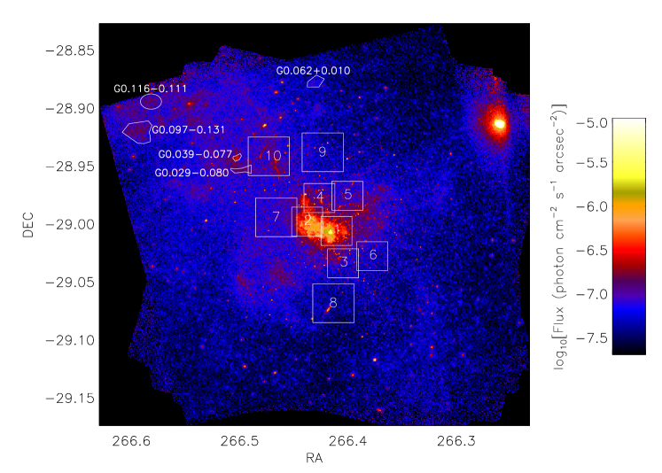
Figure 1.— Chandra image of the entire survey region, binned to 2″ resolution. The numbered boxes denote sub-images that are displayed in Figures 2 and 3.

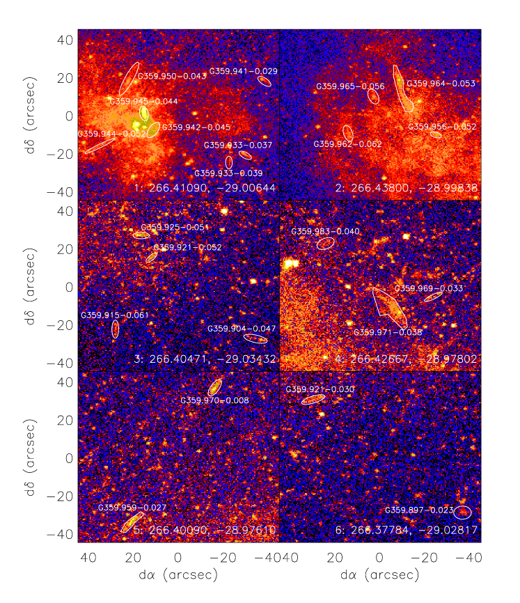
Figure 2.— Chandra images of regions near the aim-point of the survey that contain diffuse features. The coordinates of the center of each image and its number from Figure 1 are printed at the bottom of each image. The images are displayed at the full 0$\farcs$5 resolution of the detector and telescope. No smoothing has been applied. Diffuse features that are included in our catalog are outlined in white.

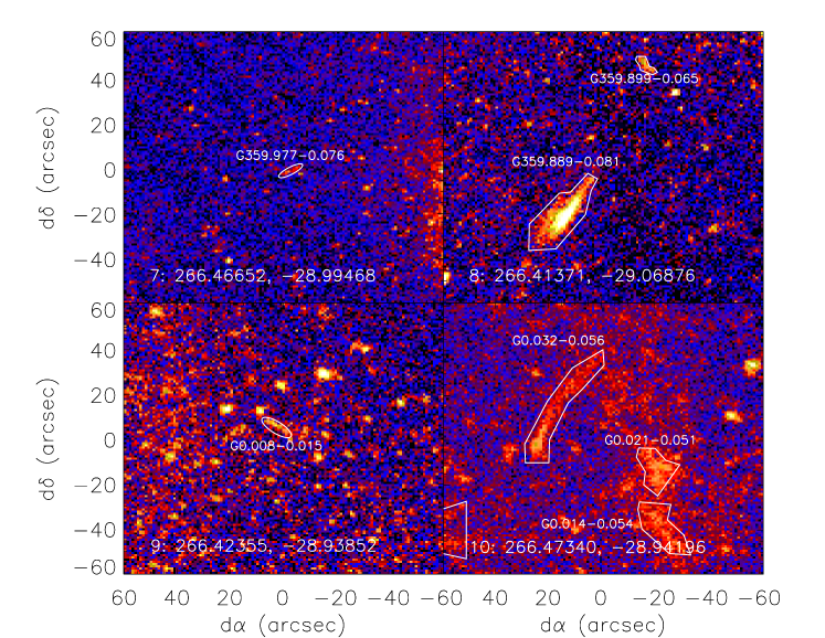
Figure 3.— Chandra images of regions near $\approx$5′ from the center of the survey that contain diffuse features, as in Figure 2. The images are binned to 1″ resolution. Diffuse features that are included in our catalog are outlined in white.

For the second search, we used the wavelet reconstruction algorithm of Starck et al. (2000). The algorithm searched for features in the 0.5–8.0 keV band image that were significant at the $\geq$3$\sigma$ level. The results of the decomposition were used to create an image of the field, and then a multi-scale vision model was used to extract the structural parameters of both point-like and extended sources. We defined as extended those sources that either (1) were clearly anisotropic, for which the ratio of the major to minor axes were greater than 1.8, or (2) appeared extended, in that their major and minor dimensions were at least 3$\sigma$ larger than the mean values at that offset from Sgr A^∗. In total, the algorithm tabulated 2709 objects, of which we identified 91 as anisotropic and 80 as unusually large, for a total of 171 extended sources.

We then compared the lists of candidate sources, and found that only 36 objects were identified using both wavelet analyses. All of the sources that were only in one of the two lists were faint, and visual inspection suggested that many were likely to be close alignments of point sources. We examined this hypothesis by extracting the average spectra of these faint features (the technique is described in §2.2). We found that the average spectra could be described as a $\Gamma=0.6$ power law absorbed by a column density of $N_{\rm H}=1\times 10^{23}$ cm^-2, along with line emission at 6.7 keV from He-like Fe with an equivalent width of 220 eV. This spectrum is similar to those of faint point-like sources in Muno et al. (2004b), which supports our hypothesis that these are not truly extended features.

At the same time, at least one feature previously identified as extended is not identified as such by either algorithm — CXOGC 174545.5–285829, the candidate neutron star suggested to be associated with Sgr A East by Park et al. (2005). Our difficulty in automatically identifying this source as diffuse probably stems from the faintness of the extended portion of its emission. Therefore, we caution that our algorithm for identifying extended features is certainly (1) not complete, in the sense that it could miss extended features, and (2) contains spurious features that are chance alignments of point sources.

We have mitigated the second problem by examining only the 34 sources that are found through both wavelet-based algorithms. The remaining 172 objects will be flagged as being “possibly extended” in an updated catalog of the point-like sources that we are preparing. In Figures 1–3, we display images with the 34 diffuse features marked. In Figure 1, we display the entire field, but for readability we only mark the locations of features with offsets of at least 6′ from Sgr A^∗, and plot boxes around portions of the field closer to the aim point that contain diffuse features. These sub-regions are displayed in Figures 2 and 3. The clustering of sources in the center of the image results mostly from the fact that the Chandra PSF is smallest near the aim point, which provides us the ability to identify $\approx$1″ features as extended.

2.2. Photometry and Spectroscopy

In order to compute the number of X-ray events received from each source, we drew by hand polygonal or elliptical regions enclosing each of the candidate diffuse features. The regions are plotted in Figures 1–3. We estimated the background counts in each region using surrounding annular regions that contained $\approx$1000 total counts, after excluding both the diffuse features and circles enclosing 92% of photons from each point source (regions excluding larger fractions of the PSF would cover the inner part of the image, leaving no events suitable for estimating a local background). We then computed approximate photon fluxes by dividing the net counts received in each of four energy bands — 0.5–2.0, 2.0–3.3, 3.3–4.7, and 4.7–8.0 keV — by the mean effective area derived using the CIAO tool mkacisarf. These energy bands were chosen to contain roughly equal numbers of counts, and so that the effective area in each energy range was roughly constant (Muno et al., 2003). In Table 3 we report the mean location, net counts, and estimated photon fluxes for each source.

To estimate the intrinsic slopes of the spectra and the absorption toward each source, we computed two hardness ratios. Following Muno et al. (2003), the ratios were defined as the fractional difference between two energy bands, $(h-s)/(h+s)$, where $h$ is the number of counts in the hard band, and $s$ is the number of counts in the soft. The soft color was calculated using $h$ as the 2.0–3.3 keV band and $s$ as the 0.5–2.0 keV band, and was most sensitive to the absorption toward each source. The hard color was calculated using $h$ as the 4.7–8.0 keV band, and $s$ as the 3.3–4.7 keV band, and provided a good measure of the intrinsic hardness of a source (Muno et al., 2004b). We list the hardness ratios in Table 3, and plot them as a function of the 0.5–8.0 keV photon fluxes in Figure 4. We also plot the hardness ratios and fluxes that we would expect for a variety of spectral shapes and luminosities and a single absorption column of $6\times 10^{22}$ cm² of gas and dust, using the thick black lines.

We find that all but one of diffuse sources have soft colors $>$$-0.175$, which implies that they are absorbed by $N_{\rm H}>4\times 10^{22}$ cm^-2 of interstellar medium. This suggests that these sources lie near or beyond the Galactic center. One source, G359.977–0.076, has a soft color of only $-0.4^{+0.3}_{-0.4}$, which implies that it is less absorbed, and probably lies within a few kpc of Earth. The luminosities of these sources, assuming they lie at $D$$=$8 kpc, are between $10^{32}$ and $10^{34}$ erg s^-1, and in general their hard colors imply that their spectra are consistent with either a power law with photon index $\Gamma\approx 1-2$, or a $kT$$>$3 keV thermal plasma. For comparison, in Figure 4 we have also plotted contours denoting the locations of the point-like sources in this diagram (Muno et al., 2004b). We find that the diffuse sources are slightly softer, with median hard color of 0.1, compared to 0.2 for the point sources.

Figure 4.— The color-intensity diagram for the diffuse features. The hard color is defined as $(h-s)/(h+s)$, where $h$ is the number of counts in the 4.7–8.0 keV band, and $s$ is the number of counts in the 3.3–4.7 keV band. The solid lines illustrate the hard colors and photon fluxes expected for thermal plasma with a range of temperatures (as marked on the right) and luminosities ($L_{\rm X}$=$10^{32}$, $10^{33}$, and $10^{34}$ erg s^-1 from left to right, for $D=8$ kpc in the 0.5–8.0 keV band), and the dotted lines are for power laws with a range of photon indices and luminosities. The contours drawn with the thin lines schematically illustrate the distribution of point-like X-ray sources in the color-magnitude diagram (Muno et al., 2004b). Diffuse features fainter than $\approx$$2\times 10^{-6}$ photons cm^-2 s^-1 have mean colors that are similar to those of the point sources, which suggests that they could be chance alignments of point sources. However, the mean color of brighter diffuse features (0.1) is lower than that of the point-like sources (0.2), which indicates they are a distinct population.

We then modeled the spectra of the brightest sources in more detail. Spectra were created by binning the source and background events over their pulse-heights. The background-subtracted spectra were then grouped such that each bin had a signal-to-noise ratio of at least 5. We found that because of their extended nature and the high background in the image, sources required $\approx$400 net counts in order to provide 4 independent spectral bins, which is required for us to constrain independently the interstellar absorption and a two-parameter continuum model. For those sources with enough signal, the observed spectra were compared with models of an absorbed power law using the chi-squared minimization implemented in XSPEC version 12.2.0 (Arnaud et al., 1996). The efficiency and energy resolution of the detector were characterized using the above effective-area function and the the energy response computed using mkacisrmf. Representative spectra of four sources are displayed in Figure 5. Most of the sources could be adequately described by these simple absorbed continuum models, but this was largely a result of the low-signal to noise. The spectral parameters are consistent with those that would be derived from Figure 4.

Figure 5.— Example spectra of diffuse features. The top panels contain the spectra in units of detector counts per second (crosses) and the best-fit model convolved with the telescope and instrument response (solid line). The bottom panels contains the residuals after subtracting the best-fit models from the data, in units of the statistical uncertainty on the observed spectra. The spectra are modeled with power-law continua and Gaussian lines (if necessary), both of which are absorbed interstellar gas and dust. Four examples are given: (a) a feature that contains a strong 6.4 keV line from low-ionization Fe, (b) a bright non-thermal feature lacking line emission, and (c) a faint source for which there is not a good constraint on the presence or absence of line emission.

However, the models did not adequately describe several of the sources with $\gtrsim$1000 net counts, and visual inspection revealed that these exhibited strong emission from low-ionization Fe at 6.4 keV (see also Park et al., 2004). Therefore, for all sources for which the spectra contained at least 5 independent spectral bins, we attempted to model the spectra as the sum of a power law plus Gaussian line emission at 6.4 keV, absorbed by the interstellar medium. If the addition of a line to the model resulted in a decrease in reduced chi-squared, we tested the significance of the added line using Markov chain Monte Carlo simulations of an $F$ test, as described in Arabadjis, Bautz, & Arabadjis (2004) and Muno et al. (2004b). The $F$ value is given by

$$F=\frac{(\chi_{s}^{2}-\chi_{c}^{2})}{(\nu_{s}-\nu_{c})}\frac{\nu_{s}}{\chi_{s}^{2}},$$ (1)

where $\chi_{s}^{2}$ and $\nu_{s}$ are the values of chi-squared and the number of degrees of freedom for the model without the line, and $\chi_{c}^{2}$ and $\nu_{c}$ are the same values for the model with a line. We simulated a set of 100–1000 spectra with parameters that were consistent with the measured parameters of the source (the Markov chain), and computed a theoretical distribution of the $F$ value under the assumption that no line was present. If the observed value of $F$ exceeded the theoretical distribution under the null hypothesis in all of 100–1000 trials, we considered a line to be detected with $>$99%–99.9% confidence. In Table 2, we list the parameters of the best-fit absorbed power law for each source we modeled, and either the measured value of the equivalent width of the 6.4 keV iron line or an upper limit to that value. We performed a similar search for the 6.7 keV line from the He-like 2–1 transition of Fe, and only found one source with such a line, G359.942–0.045 (source 2 in Table 3). The upper limits to the equivalent widths of the 6.7 keV lines from the other sources were generally 25% higher than those on the 6.4 keV lines, for the cases in which neither line was detected.

Table 2Spectral Parameters of the Diffuse Features

	Object	$N_{\rm H}$	$\Gamma$	Norm	$EW_{\rm Fe}$	$\chi^{2}/\nu$	$F_{\rm X}$	$L_{\rm X}$
							($10^{-14}$)	($10^{32}$)
		($10^{22}$ cm-2)			(eV)		(erg cm-2 s-1)	(erg s-1)
1	G359.945$-$0.044	$15.3_{-0.7}^{+0.5}$	$1.74_{-0.13}^{+0.10}$	$2.7_{-0.6}^{+0.5}\times 10^{-4}$	$<$60	187.4/175	33	66
2	G359.942$-$0.045	$9.3_{-0.6}^{+0.7}$	$2.46_{-0.16}^{+0.19}$	$1.7_{-0.5}^{+0.7}\times 10^{-4}$	$<$220	102.6/57	9	16
3	G359.944$-$0.052	$4.7_{-2.1}^{+2.0}$	$-0.17_{-0.33}^{+0.26}$	$5.0_{-3.2}^{+8.4}\times 10^{-7}$	$<$470	4.3/6	3	2
4	G359.950$-$0.043	$5.8_{-0.9}^{+2.3}$	$0.91_{-0.18}^{+0.40}$	$5.2_{-1.9}^{+9.4}\times 10^{-6}$	$<$140	10.2/12	4	4
6	G359.956$-$0.052	$3.3_{-3.2}^{+4.8}$	$-0.39_{-0.47}^{+0.95}$	$1.7_{-1.4}^{+9.0}\times 10^{-7}$	$\cdots$	1.0/1	1	1
7	G359.933$-$0.037	$14.2_{-2.0}^{+5.9}$	$1.59_{-0.29}^{+0.77}$	$1.1_{-0.6}^{+5.2}\times 10^{-5}$	$<170$	6.7/9	2	3
8	G359.941$-$0.029	$8.5_{-2.7}^{+3.4}$	$0.44_{-0.36}^{+0.57}$	$1.0_{-0.7}^{+3.0}\times 10^{-6}$	$<$180	6.6/5	2	2
9	G359.925$-$0.051	$14.6_{-2.9}^{+4.0}$	$1.77_{-0.39}^{+0.88}$	$1.2_{-0.8}^{+5.2}\times 10^{-5}$	$<$2060	5.6/5	2	3
10	G359.964$-$0.053	$9.9_{-0.8}^{+0.9}$	$1.64_{-0.15}^{+0.20}$	$6.1_{-1.8}^{+2.7}\times 10^{-5}$	$<$70	43.0/53	11	17
11	G359.965$-$0.056	$9.3_{-3.1}^{+4.5}$	$1.70_{-0.41}^{+0.75}$	$1.0_{-0.7}^{+4.2}\times 10^{-5}$	$\cdots$	6.4/3	2	3
13	G359.962$-$0.062	$4.2_{-1.6}^{+3.6}$	$0.64_{-0.39}^{+0.36}$	$1.2_{-0.8}^{+7.1}\times 10^{-6}$	$\cdots$	6.6/2	2	2
14	G359.959$-$0.027	$16.5_{-2.0}^{+3.9}$	$2.03_{-0.31}^{+0.76}$	$0.4_{-0.2}^{+1.2}\times 10^{-4}$	$<$75	6.5/12	3	6
15	G359.971$-$0.038	$12.6_{-1.7}^{+2.0}$	$1.74_{-0.25}^{+0.45}$	$4.0_{-2.0}^{+5.3}\times 10^{-5}$	$<$130	32.8/22	6	10
17	G359.921$-$0.030	$17.1_{-3.7}^{+3.6}$	$2.48_{-0.55}^{+0.87}$	$3.8_{-3.0}^{+15}\times 10^{-5}$	$<$1300	5.0/5	1	3
20	G359.904$-$0.047	2.2	–1.1	$4.4\times 10^{-8}$	$\cdots$	4.7/3	1	1
22	G359.970$-$0.008	$17.8_{-2.7}^{+3.2}$	$2.22_{-0.36}^{+0.62}$	$4.3_{-2.7}^{+9.8}\times 10^{-5}$	$<$110	5.9/11	2	6
23	G359.899$-$0.065	$26.2_{-5.1}^{+8.8}$	$1.86_{-0.85}^{+1.05}$	$1.3_{-1.1}^{+9.4}\times 10^{-5}$	$\cdots$	4.4/3	1	3
24	G359.897$-$0.023	$12.7_{-5.6}^{+4.4}$	$2.66_{-0.60}^{+1.06}$	$2.1_{-1.9}^{+15}\times 10^{-5}$	$\cdots$	0.1/1	1	2
25	G359.889$-$0.081	$29.3_{-1.1}^{+1.8}$	$1.24_{-0.18}^{+0.27}$	$1.3_{-0.4}^{+1.0}\times 10^{-4}$	$<$30	86.9/95	26	70
26	G0.014$-$0.054	$17.3_{-7.6}^{+4.0}$	$-0.11_{-0.13}^{+0.11}$	$2.0_{-4.0}^{+0.4}\times 10^{-6}$	$866_{-252}^{+300}$	11.6/14	8	11
28	G0.021$-$0.051	$15.6_{-8.5}^{+4.4}$	$-0.51_{-0.13}^{+0.11}$	$8.4_{-1.8}^{+1.8}\times 10^{-7}$	$998_{-312}^{+378}$	15.4/11	7	9
29	G0.032$-$0.056	$7.8_{-1.4}^{+1.2}$	$1.27_{-0.24}^{+0.29}$	$2.0_{-0.9}^{+1.4}\times 10^{-5}$	$<$110	26.6/27	8	10
31	G0.039$-$0.077	$10.4_{-1.8}^{+3.0}$	$0.43_{-0.12}^{+0.13}$	$6.3_{-1.0}^{+1.0}\times 10^{-6}$	$661_{-183}^{+230}$	28.8/28	11	13
32	G0.062+0.010	$9.0_{-1.4}^{+5.1}$	$1.83_{-0.36}^{+0.21}$	$3.3_{-0.8}^{+1.0}\times 10^{-5}$	$1576_{-895}^{+921}$	22.8/11	6	9
33	G0.097$-$0.131	$20.1_{-3.3}^{+2.5}$	$1.91_{-0.07}^{+0.06}$	$4.7_{-0.7}^{+0.8}\times 10^{-4}$	$1193_{-231}^{+275}$	135.4/50	48	100

Note. — All uncertainties are 1$\sigma$, determined by varying the parameter of interest until $\chi^{2}$ increased by 1.0. Limits on the equivalent width of the iron lines were only computed when there were at least 6 independent spectral bins. The flux and luminosity were computed for the 2–8 keV band.

Finally, for the 20 faintest features, we extracted their average spectrum (Fig. 6). The background was computed from an elliptical region enclosing all of the sources, but excluding the Sgr A complex. The effective area function was computed using mkwarf, and the response function using mkacisrmf. We found that the spectrum could be modeled as a $\Gamma=1.3^{+0.1}_{-0.2}$ power law absorbed by $N_{\rm H}=(1.2\pm 0.1)\times 10^{23}$ cm^-2, along with a 6.7 keV iron line with an equivalent width of 150${}^{+30}_{-70}$ eV ($\chi^{2}/\nu=92.0/88)$. The spectrum of the emission from these diffuse features is sightly steeper than that of the faint point sources (with $\Gamma=0.9$), and the He-like Fe emission is weaker (400$\pm$60 eV for point sources Muno et al., 2004b). This suggests that some, but not all, of these faint features are produced by chance alignments of point sources. Alternatively, the presence of the He-like Fe line could be explained if a diffuse thermal plasma contributes some of the flux. We therefore also modeled the emission as a non-equilibrium-ionization plasma, and found a best-fit temperature of $kT=20^{+16}_{-5}$ keV, metal abundances of $0.31^{+0.5}_{-0.5}$ solar, an ionization time scale $\tau=n_{e}t=9_{-2}^{+2}\times 10^{10}$ s cm^-3, and an absorption column of $N_{\rm H}=1.1^{+0.5}_{-0.6}\times 10^{23}$ cm^-2. We examine whether it is reasonable to presume these diffuse features are composed of hot plasma in §3.

Figure 6.— Combined spectra of the 20 faintest diffuse features, as in Fig. 5. Line emission is detected at 6.7 keV, which suggests that there is a contribution either from diffuse thermal plasma or point-like X-ray sources to these diffuse features.

2.3. Radio Fluxes

Several diffuse X-ray features elsewhere in the Galactic center region have been associated with radio sources (Sakano et al., 2003; Lu et al., 2003; Yusef-Zadeh et al., 2005). Therefore, we have examined an archival image of the Galactic center taken at 6 cm with the Very Large Array (Yusef-Zadeh & Morris, 1987) in order to search for counterparts to the X-ray features. The image is displayed in Figure 7, with the regions from Figures 1–2 overlaid. The beam size was 3$\farcs$4 by 2$\farcs$9. To compute fluxes for each feature contained within the radio image, we integrated the source flux over each feature and the background flux from an annular region around the feature, and subtracted the two. The background region had a minimum radius of 5″ for the most compact features, and was 50% bigger than the radius of the source region for the larger features. As an estimate of the uncertainty in the flux measurement, we computed the standard deviation of the flux from the source region. The fluxes and standard deviations are listed in Table 3.

Using the image in Figure 7, we obtained upper limits to the radio fluxes for the majority of the sources. The limits ranged from a few mJy at an offset of $\gtrsim$1′ from Sgr A^∗, to tens of mJy for objects located within the bright radio emission of the Sgr A complex. Only three sources have radio fluxes measured above the 5$\sigma$ level: G359.950–0.043 (source 4 in Tab 3), G359.899–0.065 (source 23 in Tab. 3, and source F in Yusef-Zadeh et al. 2005), and G359.959–0.027 (source 14 in Tab. 3). Of these, we believe that the association between the radio and X-ray emission is physical only for the latter two sources. G359.950–0.043 (source 4) lies on the “minispiral,” a feature with prominent Hydrogen recombination emission in the optical and radio, and that is therefore not hot enough to be an X-ray source on its own ($kT\sim 1$ eV; Scoville et al., 2003).

Two regions (G0.021-0.051 and G0.032–0.056) with offsets $>$4.5′ that fell within the image contained negative artifacts left by the cleaning algorithm, so we could not compute fluxes for them. Better measurements and limits would require a dedicated re-analysis of the archival VLA observations, which is beyond the scope of this paper.

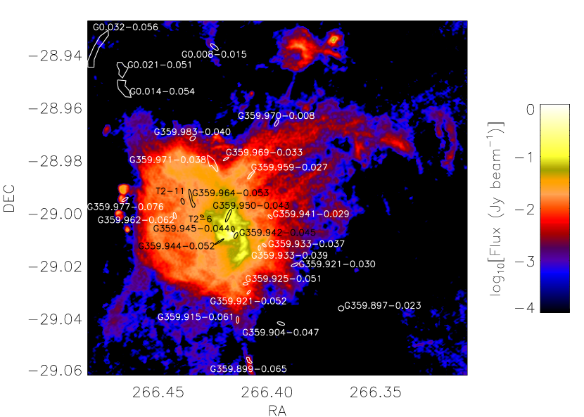
Figure 7.— Radio image taken at 6 cm with the VLA (Yusef-Zadeh & Morris, 1987), covering the central portion of the Chandra image where most of the diffuse X-ray features are found. The diffuse X-ray features are marked in either black or white. For readability, two sources are marked with their numbers from Table 2: G359.956–0.052 (source 6), and G359.965-0.056 (source 11). The beam size for the radio image is 3$\farcs$4 by 2$\farcs$9.

3. Discussion

We can roughly divide the diffuse features in the Galactic center into two groups, based on their spectral properties and sizes. Three of the four features with areas larger than 100 arcsec² exhibit strong fluorescent iron emission with equivalent widths $>$500 eV (the exception is G359.889-0.081, which we will return to shortly). These features are discussed extensively in Park et al. (2004) and Muno et al. (2007), and are produced because hard X-rays ($>$7 keV) from a transient source are being scattered by molecular gas, and causing iron to fluoresce. These features all lie in the northeast of the field. In fact, this entire quadrant of the image exhibits unusually strong diffuse Fe K-$\alpha$ emission (equivalent width 570 eV; Muno et al., 2004a). The features that we identify in this paper are simply the brightest manifestations of this pervasive scattered and fluorescent emission, and they probably trace regions of molecular gas with the highest optical depth. It is notable, however, that similar features are not seen toward other clouds with similarly high optical depth, particularly those with velocities of $+$20 km s^-1 and $+$40 km s^-1 just to the east of Sgr A^∗ (e.g., Güsten, Walmsley, & Pauls 1981; Oka et al. 1998). The clouds that do not exhibit fluorescent emission are slightly in the foreground of the field, as they are seen to cast a shadow in the number of X-ray sources along their lines of sight (Muno et al., 2003). The clouds without associated X-ray emission must not intersect the light-front of the transient that illuminated the fluorescent features.

The features with surface area $<$100 arcsec² either exhibit no evidence for iron emission at 6.4 keV, or are too faint for such emission to be detected. Based on their spectra, the X-ray emission from these features must either originate from a hot thermal plasma ($kT\gtrsim 7$ keV; Fig. 4), or from non-thermal processes such as synchrotron or inverse-Compton scattering. As we describe below, previous work on individual features suggests that they have a variety of origins. This is the first paper to provide a comprehensive compilation of their properties. For brevity, we will refer to the features without obvious fluorescent iron emission as “streaks.” Below, we speculate about their natures.

3.1. Thermal Shocks

The possibility that some of the features are thermal is suggested by the detection of the 6.7 keV line from He-like iron in the combined spectra of the faint diffuse features (Fig. 6). However, this hypothesis requires that some mechanism must be found to confine the plasma. For a characteristic temperature of $\approx$7 keV, and a luminosity of $L_{\rm X}=10^{33}$ erg s^-1 (2–8 keV), the emission measure is $\int n_{e}n_{\rm H}dV\approx n_{e}^{2}V=1\times 10^{56}$ cm^-3, where $n_{e}$ is the electron density, $n_{\rm H}$ is the hydrogen density, and $V$ is the volume of the emitting region. The sizes of these features are typically $\Omega\approx 20-100$ arcsec², which for $D$$=$8 kpc corresponds to projected areas of $A\approx 0.03-0.15$ pc². If we assume that the volume is given by $V=A^{3/2}$, then the electron density of the plasma is $n_{e}=13\Omega_{50}^{-3/4}L_{\rm X,33}^{1/2}$ cm^-3, where $\Omega_{50}$ is normalized to 50 arcsec², and $L_{\rm X,33}$ to $10^{33}$ erg s^-1 (2–8 keV). Therefore, the pressure is $P=1\times 10^{-7}\Omega_{50}^{-3/4}L_{\rm X,33}^{1/2}$ erg cm^-3. This pressure is $\approx$300 times larger than that of the diffuse, $kT\approx 0.8$ keV plasma in the Galactic center ($3\times 10^{-10}$ erg cm^-3), and 50 times larger than the putative 8 keV plasma there ($2\times 10^{-9}$ erg cm^-3; Muno et al., 2004a). Magnetic fields would have to be strong to confine this plasma, $B=2\Omega_{50}^{-3/8}L_{\rm X,33}^{1/4}$ mG. These fields strengths are thought to be present within radio-emitting filaments toward the Galactic center (Morris & Serabyn, 1996), but the average field at the Galactic center may be significantly lower (e.g., LaRosa et al., 2005). Thermal features could also be produced by shocks with velocities of $\sim$$(4kT/3\mu m_{p})^{1/2}$=1200 km s^-1 (where $m_{p}$ is the proton mass and $\mu$=0.5 for a plasma of electrons and protons). However, there are no obvious candidates for the sources of the energy powering these putative shocks; they are not arranged as part of a shell as would be expected if they originate from a supernova (and the lack of metal lines would be puzzling), and the known massive stars in the region are mostly located within 30″ of Sgr A*, which is several parsecs in projection from these features (e.g., Krabbe et al., 1995; Paumard et al., 2006).

3.2. Supernova Remnants

Given the problems with assuming that these features are thermal sources, we follow other authors and suggest that the majority of these features are non-thermal. A few of the X-ray streaks appear to be non-thermal particles accelerated in shocks where supernova remnants impact the interstellar medium. It has been noted by several authors that G359.889–0.081 and G359.899–0.065 (sources 25 and 23 in Table 3) lie on part of a shell-like feature seen in radio maps (Sakano et al., 2003; Lu et al., 2003; Yusef-Zadeh et al., 2005). These features are coincident with the brightest parts of the radio-emitting shell, which are referred to as E and F by Ho et al. (1985, and Fig. 7). We also find four filamentary features associated with the Sgr A East supernova remnant, G359.962–0.062, G359.965–0.056, G359.964–0.053, and G359.956–0.052 (sources 6, 10, 11, and 13 in Table 3). Of these features associated with supernova remnants, we can put strict upper limits to the equivalent width of iron emission for G359.956-0.052 and G359.889–0.081, $<$70 and $<$30 eV, respectively, which strongly suggests that they are non-thermal. The X-rays are probably synchrotron emission from TeV electrons (Yusef-Zadeh et al., 2005), which could occur in parts of remnants where the shock velocity is high and the ambient density is low, so that particles are efficiently accelerated (e.g., Vink et al., 2006). Supernova shocks therefore can explain 5 of the 26 streaks.

3.3. Non-Thermal Radio Filaments

At least one non-thermal radio filament has been identified with X-ray emission in the central 100 pc of the Galaxy, but outside of our deep images of the central 20 pc: G 359.54+0.18 (Lu et al., 2003). This confirmed non-thermal filament produces a flux density of 150 mJy at 6 cm over the region that also emits X-rays. Assuming an $\alpha=-0.8$ spectrum, the estimated radio luminosity of G 359.54+0.18 between $10^{7}$ Hz and $10^{11}$ Hz is $L_{\rm R}=5\times 10^{32}$ erg s^-1, compared to an X-ray luminosity of $L_{\rm X}=2.4\times 10^{33}$ erg s^-1 (0.2–10 keV Lu et al., 2003). In our image, however, only one diffuse feature that is not associated with a supernova remnant has a firm radio counterpart, G359.959–0.027 (source 14 in Table 3). Its X-ray luminosity is $L_{\rm X}=6\times 10^{32}$ erg s^-1 (2–8 keV). In Fig. 7 (Yusef-Zadeh & Morris, 1987), the feature has a flux density of $20\pm 3$ mJy, which for the same assumed radio spectrum as above implies $L_{\rm R}=2\times 10^{31}$ erg s^-1. A second nearby feature with a similar size, spectrum, and even orientation, G359.970–0.008 (Figure 2, panel 5; source 22 in Table 3), also has a marginal radio counterpart with a flux of $1.2\pm 0.4$ mJy. For this source we find $L_{\rm X}=6\times 10^{32}$ erg s^-1 (2–8 keV) and $L_{\rm R}\approx 9\times 10^{29}$ erg s^-1. Therefore, a couple of the streaks could be counterparts to non-thermal radio filaments, although the relative amount of radio and X-ray flux appears highly variable.

3.4. Pulsar Wind Nebulae

The final conventional explanation for the X-ray streaks is that they could be pulsar wind nebulae. Two candidate pulsar wind nebulae in this field have been discussed in the literature. Wang et al. (2006) have demonstrated that the spectral and morphological properties of G359.945–0.044 resemble a pulsar wind nebula, and have suggested that it is the source of the TeV emission that originates near Sgr A^∗ (Aharonian et al., 2004). This source is included in our catalog. Park et al. (2005) have identified the point-source CXOGC J174545.5–285829 as another candidate pulsar based on its featureless non-thermal spectrum, its lack of long-term variability, and the detection of a faint extended tail that may represent a bow shock formed by the wind nebula. This object is not in our catalog, because the faint nebulosity was not identified by our wavelet algorithms (see §2.1). From this new work, one bright feature has a morphology that makes it an especially attractive candidate to be a pulsar wind nebulae: G 0.032–0.056 (source 29 in Table 3), which has a bright head producing about half its flux, and a long tail that curves to the northwest.

Pulsar wind nebulae are formed when a wind of particles that is powered by the rotational energy of the neutron star encounters the ISM. The resulting shock accelerates the particles further, causing them to radiate synchrotron emission (see Gaensler & Slane, 2006, for a review). These wind nebulae have diverse morphologies, which depend upon how the pulsar wind interacts with the surrounding supernova remnant, how far the pulsar travels during the lifetime of the electrons in the wind nebula, and whether the pulsar is moving supersonically with respect to the ISM. In the Galactic center, few of the pulsars are likely to be moving highly supersonically. Most of the region is probably suffused with hot $kT\approx 0.8$ keV plasma with densities of $n\approx 0.1$ cm^-3, which implies that the sound speed of the ISM is $\approx$500 km s^-1 (Muno et al., 2004a). In contrast, the mean three-dimensional velocities of known radio pulsars are $\approx$400 km s^-1 (e.g., Hobbs et al., 2005; Faucher-Giguère & Kaspi, 2006), and only 2 of 169 pulsars in Hobbs et al. (2005) have measured transverse velocities $>$800 km s^-1, which, assuming the velocities are isotropic, would translate to expected three-dimensional velocities $>$1000 km s^-1. Pulsars will only be highly supersonic (Mach numbers $>$2) in regions of the ISM that are dense and cool, such as near molecular clouds. Therefore, we would not expect bow-shock nebulae to be common (although see Park et al., 2005). Nonetheless, the complex morphologies we observe could be explained by interactions between wind nebulae and unseen supernova remnants (e.g., Gaensler et al., 2003), or if the proper motion of the pulsar moves the particle acceleration region faster than the electrons can cool (e.g., SN G371.1-1.1 in Gaensler & Slane, 2006). The characteristic sizes of known pulsar nebulae are between $10^{17}$ and $10^{19}$ cm (Cheng, Taam, & Wang 2004), which at the Galactic center ($D$=8 kpc) would have angular sizes of 0$\farcs$8–80″. This bounds the sizes of the features we observe.

Moreover, the X-ray luminosities of the diffuse features in the Galactic center are consistent with those of known pulsar wind nebulae. Galactic pulsar wind nebulae have X-ray luminosities that are as large as $\sim$$10^{37}$ erg s^-1 (2–10 keV); typically, $\sim$$10^{-3}$ of the spin-down energy $\dot{E}$ is emitted as X-rays (e.g., Becker & Trümper, 1997; Cheng et al., 2004; Gaensler & Slane, 2006). The diffuse features in our survey all have luminosities of $L_{\rm X}\sim 10^{32}$–$10^{34}$ erg s^-1, which would imply spin-down luminosities of $\dot{E}\sim 10^{35}-10^{37}$ erg s^-1. There are $\approx$86 known pulsars with $\dot{E}$ in this range. Most of these energetic pulsars have ages $\lesssim$$10^{5}$ years, although 7 of $\sim$100 known recycled millisecond pulsars have $\dot{E}$ this high (Manchester et al., 2005).

Many Galactic pulsar wind nebulae are luminous at radio wavelengths, and yet we find that most of our X-ray sources do not have radio counterparts. The limits to their flux densities at 6 cm are $\lesssim$3 mJy (Tab. 3 and Fig. 7). If we assume a standard pulsar wind spectrum with logarithmic slope $\alpha=-0.3$ between $10^{7}$ and $10^{11}$ Hz, our typical limit of 3 mJy corresponds to $L_{\rm R}\sim 10^{31}$ erg s^-1, or between $10^{-1}$ and $10^{-3}$ of the X-ray luminosity. This would translate to $\sim(10^{-4}-10^{-6})\dot{E}$. For comparison, the youngest, most energetic Galactic pulsars are detected with $L_{\rm R}\sim 10^{-4}\dot{E}$. However, for $\dot{E}\lesssim 10^{36}$ erg s^-1 a few pulsars have $L_{\rm R}\lesssim 10^{-5}\dot{E}$ (Frail & Scharringhausen, 1997; Gaensler et al., 2000): of $\approx$30 pulsars that have been reasonably well-studied at X-ray (Becker & Trümper, 1997; Cheng et al., 2004) and radio (Frail & Scharringhausen, 1997; Gaensler et al., 2000) wavelengths, five stand out as having wind nebulae with $L_{\rm X}>10^{32}$ erg s^-1 and $L_{\rm R}\lesssim(10^{-5}-10^{-7})\dot{E}$: PSR B1046–58 (Gonzales et al., 2006), PSR B1823–13 (Gaensler et al., 2003), PSR B0355+54 (McGowan et al., 2006), PSR B1706-44 (Gotthelf, Halpern, & Dodson, 2002; Romani et al., 2005), and possibly PSR J1105–6107 (Gotthelf & Kaspi, 1998). The sources in our sample that are either bright in X-rays or that have strict limits to their radio fluxes would have to be analogous to these radio-faint pulsars.

Given that the lack of radio detections can be reconciled plausibly with the known properties of pulsars, we next examine whether we should expect enough energetic pulsars in the Galactic center to account for the number of diffuse features that we observe. Wang et al. (2005) and Cheng et al. (2006) have considered whether recycled millisecond pulsars in the Galactic center could contribute to these X-ray features. Based on the inferred population of Galactic millisecond pulsars (Lyne et al., 1998), they estimate that $\sim$200 could be present in our survey region. If, based on the catalog of Manchester et al. (2005), $\sim$10% of the millisecond pulsars have $\dot{E}>10^{35}$ erg s^-1, they also could contribute $\sim$20 objects to the diffuse features at the Galactic center. These pulsars will generally be traveling rather slow ($v$$\sim$130 km s^-1 Lyne et al., 1998), relative to the sound speed of the $\approx$0.8 keV plasma that takes up most of the volume of the ISM at the Galactic center (Muno et al., 2004a), but they could form extended nebulae if they encounter regions of the ISM with relatively low sound velocities ($kT$$\lesssim$0.1 keV). The filling factor of this cooler ISM is unknown, but if it is $\gtrsim$10%, a handful of millisecond pulsars could produce extended diffuse features.

Most of the known energetic pulsars with wind nebulas are young, and still interacting with their supernova remnants. We concentrate on these as the best candidates for the diffuse X-ray features. Figer et al. (2004) modeled the infrared color-magnitude diagrams of stars in several fields toward the Galactic center, and, assuming an initial mass function (IMF) of the form $dN\propto M^{-0.9}$ for stars with masses between 0.1 $M_{\odot}$ and 120$M_{\odot}$, concluded that the star formation rate in the inner 30 pc of the Galaxy is 0.02 $M_{\odot}$ yr^-1. If we assume that radio pulsars form from stars with initial masses between 8 and 30 $M_{\odot}$ (e.g., Brazier & Johnston, 1999; Heger et al., 2003, but see Figer et al. 2005; Muno et al. 2006), then they would form at a rate of $2\times 10^{-4}$ yr^-1.

However, the supernovae that produce pulsars provide them with kicks, so the loss of pulsars as they move out of the Galactic center will also limit the number of pulsar wind nebulae observable there (e.g., Cordes & Lazio, 1997). There is still debate as to the three-dimensional velocity distribution of pulsars (e.g., Arzoumanian, Chernoff, & Cordes, 2002; Hobbs et al., 2005; Faucher-Giguère & Kaspi, 2006), so we have adopted a simplified approach to estimate the number of pulsars remaining within the 8′ (20 pc) radial bound of our image, based upon the observed tangential velocities for 169 radio pulsars that were tabulated by Hobbs et al. (2005). We assume that a pulsar would remain in our image if the product of its tangential velocity $v$ and its lifetime $t$ is less than $D$=20 pc. Using the data in Hobbs et al. (2005), we can compute the fraction of known pulsars in that sample that have traveled a projected distance $D$$<$20 pc at a given age $t$, which we call $f(t)$. If pulsars are born at a constant rate $R$=$2\times 10^{-4}$ yr^-1 and are bright pulsar wind nebulae for a time $t_{\rm bright}$, then the number of nebulae in our image is roughly

$$N=R\int^{t_{\rm bright}}_{0}f(t)dt.$$ (2)

For $t_{\rm bright}$=100 kyr we find that only pulsars with $v$$>$200 km s^-1 may have time to escape, and that out of 20 pulsars born, roughly 14 would remain within our image. If $t_{\rm bright}$=300 kyr, pulsars with $v$¿70 km s^-1 may escape, so that 29 out of 60 pulsars would remain. In this estimate, we have not considered that some pulsars will be gravitationally bound to the Galactic center. If we use the enclosed mass in Genzel et al. (1996), the escape velocity from a radius of 10 pc is only $v_{\rm esc}\approx 200$ km s^-1. Therefore, if $t_{\rm bright}$ is significantly longer than 100 kyr, then the fraction of pulsars retained in the Galactic center would be larger than we estimate (66% of pulsars have tangential velocities smaller than 200 km s^-1, although many of these will have larger three-dimensional velocities). For comparison, if we consider candidate pulsar wind nebulae to be those features that (1) exhibit no evidence for iron emission, and (2) are not obviously associated with supernova remnants already detected in the radio, then there are also $\sim$20 of them in our image. This is consistent with the numbers we expect if pulsars produce wind nebulae for 100–300 kyr after their birth.

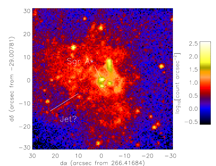
Figure 8.— Chandra image of the central 30″ around Sgr A^∗, at 0$\farcs$5 resolution. The white line pointing toward the southeast away from Sgr A^∗ runs parallel to a jet-like feature that was identified using our wavelet analysis (G359.944–0.052; source 3 in Tab. 3). The jet becomes noticeable at at an offset of $\approx$10″ from Sgr A^∗.

3.5. A Jet from Sgr A^∗?

Finally, we note that one of the X-ray features may be a jet produced by Sgr A^∗, G359.944–0.052 (source 3 in Table 3). We highlight this source in particular in Figure 8. The object is about 15″ long, and is unresolved along its short axis. Our hypothesis that it is a jet is motivated by the fact that it position angle points within 2^∘ of Sgr A^∗. From a visual inspection of the rest of our image, we find only one candidate feature that is similarly long and thin (located at $\alpha,\delta$= 266.37688, –29.04517), but this feature is not picked up by the automated wavelet search based on the work of Starck et al. (2000) because it is half as bright as G359.944–0.052. The candidate jet is found by both of our wavelet algorithms, so we believe this feature is unlikely to be an artifact produced by a chance alignment of point sources, or by Poisson variations in the diffuse background. The feature has a flat spectrum of slope $\Gamma=-0.2\pm 0.3$ and an absorption column within 1$\sigma$ of the average toward the Galactic center, $N_{\rm H}=(5\pm 2)\times 10^{22}$ cm^-2. Its luminosity is $L_{\rm X}=2\times 10^{32}$ erg s^-1 (2–8 keV).

The candidate jet is not detected in the radio, with an upper limit of $<$45 mJy at 6 cm (5 GHz). The radio upper limit is not constraining because the feature lies along the line-of-sight toward bright, diffuse radio emission. The relative strength of the radio and X-ray emission from the synchrotron-emitting jets of quasars can be quantified using the logarithmic slope $\alpha_{\rm RX}=-\log(S_{\rm X}/S_{\rm R})/\log(\nu_{\rm X}/\nu_{\rm R})$, where $S_{\rm X}$ and $S_{\rm R}$ and the X-ray and radio flux densities, and $\nu_{\rm X}$ and $\nu_{\rm R}$ are the frequencies at which the flux densities are computed. From the values in Table 2, $S_{\rm X}=0.3$ nJy at $\nu_{\rm X}=2.4\times 10^{17}$ Hz (1 keV). Therefore, we can only constrain $\alpha_{\rm RX}<1.1$. For comparison, the quasars in the sample of Marshall et al. (2005) have $\alpha_{\rm RX}$ between 0.9 and 1.1. Therefore, one would need radio observations with a sensitivity of $<$1 mJy to make a useful comparison between the putative jet feature near Sgr A^∗ and quasar jets. Further observations are warranted to determine whether G359.944–0.052 is a jet of synchrotron-emitting particles that is flowing away from Sgr A^∗.

4. Conclusions

There are several processes that appear to produce diffuse X-ray features in the Galactic center: X-rays scatter off of gas in molecular clouds, and cause them to fluoresce; supernova shocks produce X-ray emitting, TeV electrons when they propagate through low-density ISM; and non-thermal radio filaments produce X-rays through a mechanism that is still not understood.

However, we propose that the majority of the diffuse X-ray features are pulsar wind nebulae. A significant number of pulsars are expected at the Galactic center, but because of the high dispersion measure along the line of sight, only two have so far been reported there in the radio (Johnston et al., 2006). X-ray identifications of pulsar wind nebulae bypass the problem of the dispersion measure, and in addition are sensitive to pulsars that are not beamed toward our line of sight. Therefore, the identification of $\approx$20 X-ray features that are candidate pulsar wind nebulae is consistent with a basic prediction about the number of massive stars that have recently ended their lives in the Galactic center. However, at the moment we lack identificaations of most of these features at other wavelengths, so further multi-wavelength studies are required to confirm our hypotheses.

Table 3Diffuse Features in the Central 20 pc of the Galaxy

Number	Object	RA	DEC	Area	Offset	Live Time	Net Counts	$\log{P_{\rm back}}$	HR0	HR2	$F_{\rm X}$	$S_{\rm 5~{}GHz}$
		(degrees, J2000)		arcsec2	(arcmin)	(ks)					($10^{-7}$ ph cm-2 s-1)	(mJy)
1	G359.945-0.044	$266.41574$	$-29.00617$	22	0.1	927	$10357.5^{+101.8}_{-101.8}$	$<$–99.0	$0.89_{-0.01}^{+0.01}$	$0.11_{-0.01}^{+0.01}$	419.6	$<$100
2	G359.942-0.045	$266.41443$	$-29.00857$	28	0.1	927	$3650.0^{+60.4}_{-60.4}$	–10.8	$0.84_{-0.01}^{+0.01}$	$-0.16_{-0.03}^{+0.03}$	132.3	$<$30
3	G359.944-0.052	$266.42200$	$-29.01091$	20	0.3	927	$695.9^{+62.7}_{-62.7}$	–11.1	$1.00_{-0.13}$	$0.20_{-0.05}^{+0.05}$	29.2	$<$45
4	G359.950-0.043	$266.41788$	$-29.00109$	55	0.4	927	$1296.0^{+36.0}_{-36.0}$	–8.9	$0.88_{-0.02}^{+0.02}$	$-0.01_{-0.05}^{+0.05}$	50.6	210$\pm$30
5	G359.933-0.039	$266.40372$	$-29.01335$	15	0.8	927	$200.4^{+32.6}_{-31.6}$	–3.4	$0.29_{-0.77}^{+0.28}$	$-0.03_{-0.12}^{+0.10}$	8.1	$<$3
6	G359.956-0.052	$266.43002$	$-29.00123$	10	0.8	927	$295.5^{+41.0}_{-40.2}$	–3.1	$1.00_{-0.55}$	$0.14_{-0.09}^{+0.08}$	12.7	$<$9
7	G359.933-0.037	$266.40140$	$-29.01229$	13	0.9	927	$542.9^{+44.0}_{-44.0}$	–17.2	$0.72_{-0.08}^{+0.06}$	$0.09_{-0.05}^{+0.05}$	22.8	$<$5
8	G359.941-0.029	$266.39868$	$-29.00148$	17	1.0	927	$430.5^{+41.7}_{-40.9}$	–11.7	$1.00_{-0.32}$	$0.19_{-0.05}^{+0.05}$	18.7	$<$2
9	G359.925-0.051	$266.41000$	$-29.02688$	19	1.2	927	$427.7^{+41.0}_{-40.6}$	–7.5	$1.00_{-0.42}$	$0.06_{-0.06}^{+0.06}$	18.1	$<$2
10	G359.964-0.053	$266.43475$	$-28.99465$	76	1.2	927	$3424.4^{+58.5}_{-58.5}$	–41.9	$0.82_{-0.01}^{+0.01}$	$0.01_{-0.02}^{+0.02}$	151.1	11$\pm$3
11	G359.965-0.056	$266.43893$	$-28.99563$	29	1.4	927	$568.7^{+60.7}_{-60.4}$	–6.8	$1.00_{-0.22}$	$-0.12_{-0.09}^{+0.08}$	22.4	$<$2
12	G359.921-0.052	$266.40854$	$-29.03010$	12	1.4	927	$169.2^{+28.4}_{-26.9}$	–3.6	$1.00_{-0.40}$	$0.29_{-0.09}^{+0.08}$	7.5	$<$1
13	G359.962-0.062	$266.44254$	$-29.00101$	26	1.4	927	$523.9^{+59.0}_{-59.0}$	–1.1	$1.00_{-0.15}$	$-0.07_{-0.10}^{+0.09}$	20.3	2$\pm$1
14	G359.959-0.027	$266.40738$	$-28.98546$	34	1.4	927	$773.7^{+27.8}_{-27.8}$	–32.7	$1.00_{-0.22}$	$0.08_{-0.04}^{+0.04}$	33.6	20$\pm$3
15	G359.971-0.038	$266.42542$	$-28.98094$	148	1.7	927	$1786.7^{+42.3}_{-42.3}$	–19.8	$0.64_{-0.07}^{+0.06}$	$0.01_{-0.04}^{+0.04}$	71.4	$<$10
16	G359.969-0.033	$266.41895$	$-28.97952$	17	1.7	927	$207.4^{+31.5}_{-30.6}$	–5.6	$1.00_{-0.47}$	$0.28_{-0.08}^{+0.07}$	9.0	$<$1
17	G359.921-0.030	$266.38730$	$-29.01968$	30	1.7	927	$391.8^{+39.1}_{-38.9}$	–12.7	$1.00_{-0.41}$	$-0.03_{-0.07}^{+0.06}$	15.7	$<$1
18	G359.915-0.061	$266.41370$	$-29.04057$	22	2.0	927	$192.3^{+29.5}_{-28.3}$	–15.2	$-9.00$	$0.54_{-0.05}^{+0.04}$	10.0	1.8$\pm$0.7
19	G359.983-0.040	$266.43433$	$-28.97174$	35	2.4	927	$139.6^{+36.5}_{-36.0}$	–0.5	$0.51_{-0.19}^{+0.12}$	$-0.11_{-0.33}^{+0.23}$	5.4	$<$1
20	G359.904-0.047	$266.39368$	$-29.04198$	32	2.4	927	$296.5^{+35.3}_{-34.6}$	–6.7	$1.00_{-0.39}$	$0.28_{-0.06}^{+0.05}$	13.2	$<$0.2
21	G359.977-0.076	$266.46542$	$-28.99490$	26	2.7	927	$164.4^{+29.9}_{-29.0}$	–1.6	$-0.35_{-0.39}^{+0.28}$	$0.19_{-0.13}^{+0.11}$	6.5	$<$4
22	G359.970-0.008	$266.39569$	$-28.96591$	30	2.7	927	$640.7^{+47.1}_{-46.7}$	–32.6	$1.00_{-0.26}$	$0.11_{-0.04}^{+0.04}$	28.1	1.2$\pm$0.4
23	G359.899-0.065	$266.40851$	$-29.05584$	30	2.9	927	$222.2^{+30.1}_{-28.6}$	–10.7	$0.41_{-0.32}^{+0.18}$	$0.42_{-0.06}^{+0.05}$	11.0	6$\pm$1
24	G359.897-0.023	$266.36603$	$-29.03623$	42	3.2	927	$233.1^{+32.9}_{-31.3}$	–2.3	$0.45_{-0.15}^{+0.11}$	$-0.03_{-0.11}^{+0.10}$	9.2	$<$0.4
25	G359.889-0.081	$266.41791$	$-29.07335$	432	3.9	927	$5364.7^{+73.2}_{-73.2}$	$<$-99.0	$0.45_{-0.12}^{+0.09}$	$0.45_{-0.01}^{+0.01}$	281.9	$\cdots$
26	G0.014-0.054	$266.46631$	$-28.95223$	260	4.2	927	$1551.1^{+39.4}_{-39.4}$	–28.4	$-0.04_{-0.89}^{+0.39}$	$0.54_{-0.02}^{+0.02}$	78.1	$<$0.6
27	G0.008-0.015	$266.42432$	$-28.93708$	51	4.3	927	$223.2^{+34.2}_{-32.9}$	–3.1	$0.24_{-0.34}^{+0.21}$	$-0.11_{-0.13}^{+0.11}$	9.2	1.6$\pm$0.5
28	G0.021-0.051	$266.46741$	$-28.94492$	190	4.6	927	$1326.7^{+36.4}_{-36.4}$	–27.8	$1.00_{-0.69}$	$0.61_{-0.02}^{+0.02}$	69.2	$\cdots$
29	G0.032-0.056	$266.47849$	$-28.93840$	429	5.3	927	$2305.2^{+48.0}_{-48.0}$	–30.8	$1.00_{-0.21}$	$0.02_{-0.04}^{+0.04}$	100.9	$\cdots$
30	G0.029-0.080	$266.50043$	$-28.95345$	838	5.5	927	$1398.2^{+37.4}_{-37.4}$	–18.3	$1.00_{-0.74}$	$0.49_{-0.04}^{+0.04}$	73.0	$\cdots$
31	G0.039-0.077	$266.50354$	$-28.94300$	333	6.0	927	$2424.8^{+49.2}_{-49.2}$	–33.5	$0.59_{-0.10}^{+0.07}$	$0.29_{-0.02}^{+0.02}$	118.4	$\cdots$
32	G0.062+0.010	$266.43198$	$-28.87782$	1187	7.8	927	$1566.5^{+39.6}_{-39.6}$	–14.7	$0.72_{-0.06}^{+0.05}$	$0.06_{-0.06}^{+0.05}$	75.9	$\cdots$
33	G0.097-0.131	$266.59061$	$-28.92188$	4181	10.5	563	$5246.9^{+72.4}_{-72.4}$	$<$-99.0	$0.12_{-0.44}^{+0.25}$	$0.21_{-0.02}^{+0.02}$	529.0	$\cdots$
34	G0.116-0.111	$266.58212$	$-28.89475$	2257	11.0	574	$1291.3^{+35.9}_{-35.9}$	–7.3	$0.18_{-0.41}^{+0.23}$	$0.24_{-0.07}^{+0.06}$	121.6	$\cdots$

Note. — The object name is constructed from the Galactic coordinates in degrees. The position is given in degrees as the right ascension and declination, at the epoch J2000. The area is that of the extraction region in Figures 1–3. The offset is from Sgr A^∗. The live time is the amount of time for which the target was in the field of view of the detector. The net counts are in the 0.5–8.0 keV band, and the uncertainties are 1$\sigma$. $P_{\rm back}$ is the probability that the spectrum of the feature is the same as that of the background, estimated via a KS test. The hardness ratios are defined as $(h-s)/(h+s)$. For HR0, $h$ is the 2.0–3.3 keV band, and $s$ is the 0.5–2.0 keV band. For HR2, $h$ is the 4.7–8.0 keV band, and $s$ is the 3.3–4.7 keV band. HR1 is not used. The flux is the observed value from the 0.5–8.0 keV band. The radio fluxes are taken from the 6 cm (5 GHz) image in Figure 7.

References

- Aharonian et al. (2004) Aharonian, F. et al. 2004, A&A, 425, L13
- Arabadjis et al. (2004) Arabadjis, J. S., Bautz, M. W., & Arabadjis, G. 2004, ApJ, 617, 303
- Arnaud et al. (1996) Arnaud, K.A., 1996, Astronomical Data Analysis Software and Systems V, eds. Jacoby G. and Barnes J., p17, ASP Conf. Series volume 101
- Arzoumanian, Chernoff, & Cordes (2002) Arzoumanian Z., Chernoff D. F., & Cordes J. M., 2002, ApJ, 568, 289
- Baganoff et al. (2003) Baganoff, F. K. et al. 2003, ApJ, 591, 891
- Becker & Trümper (1997) Becker, W. & Trümper, J. 1997, A&A, 326, 682
- Bertin & Arnouts (1996) Bertin, E. & Arnouts, S. 1996, A&A, 117, 393
- Brazier & Johnston (1999) Brarzier, K. T. S. & Johnston, S. 1999, MNRAS, 305, 671
- Bykov (2002) Bykov, A. M. 2002, A&A, 390, 327
- Cheng et al. (2004) Cheng, K. S., Taam, R. E., & Wang, W. 2004, ApJ, 617, 480
- Cheng et al. (2006) Cheng, K. S., Taam, R. E., & Wang, W. 2006, ApJ, 641, 427
- Cordes & Lazio (1997) Cordes, J. M. & Lazio, T. J. W. 1997, ApJ, 475, 557
- Faucher-Giguère & Kaspi (2006) Faucher-Giguère, C.-A. & Kaspi, V. M. 2006, ApJ, 643, 332
- Figer et al. (2004) Figer, D. F., Rich, R. M., Kim, S. S., Morris, M., & Serabyn, E. 2004, ApJ, 610, 317
- Frail & Scharringhausen (1997) Frail, D. A., & Scharringhausen, B. R. 1997, ApJ, 480, 364
- Freeman et al. (2002) Freeman, P. E., Kashyap, V., Rosner, R., & Lamb, D. Q. 2002, ApJS, 138, 185
- Gaensler & Slane (2006) Gaensler, B. M. & Slane, P. O. 2006, ARA&A, 44, 17
- Gaensler et al. (2000) Gaensler, B. M., Stappers, B. W., Frail, D. A., Moffat, D. A., Johnston, S., & Chatterjee, S. 2000, MNRAS, 318, 58
- Gaensler et al. (2003) Gaensler, B. M., Schulz, N. S., Kaspi, V. M., Pivovaroff, M. J., & Becker, W. E. 2003, ApJ, 588, 441
- Genzel et al. (1996) Genzel, R., Thatte, N., Krabbe, A., Kroker, H., & Tacconi-Garman, L. E. 1996, ApJ, 472, 153
- Gonzales et al. (2006) Gonzales, M. E., Kaspi, V. M., Pivovaroff, M. J. & Gaensler, B. M. 2006, ApJ, 652, 569
- Gotthelf, Halpern, & Dodson (2002) Gotthelf, E. V., Halpern, J. P., & Dodson, R. 2002, ApJ, 567, L125
- Gotthelf & Kaspi (1998) Gotthelf, E. V. & Kaspi, V. .M. 1998, ApJ, 497, 429
- Güsten et al. (1981) Güsten, R., Walmsley, C. M., & Pauls, T. 1981, A&A, 103, 197
- Heger et al. (2003) Heger, A., Fryer, C. L., Woosley, S. E., Langer, N., & Hartmann, D. H. 2003, ApJ, 591, 288
- Ho et al. (1985) Ho, P. T. P., Jackson, J. M., Barret, A. H., & Armstrong, T. J. 1985, ApJ, 288, 575
- Hobbs et al. (2005) Hobbs, G., Lorimer, D. R., Lyne, A. G., & Kramer, M. 2005, MNRAS, 360, 974
- Johnston et al. (2006) Johnston, S., Kramer, M., Lorimer, D. R., Lyne, A. G., McLaughlin, M., Klein, B., & Manchester, R. N. 2006, MNRAS, 373, L6
- Krabbe et al. (1995) Krabbe, A. et al. 1995, ApJ, 447, L95
- Kroupa (2002) Kroupa, P. 2002, Science, 295, 82
- Koyama et al. (1996) Koyama, K., Maeda, Y., Sonobe, T., Takeshima, T., Tanaka, Y., & Yamauchi, S. 1996, PASJ, 48, 249
- LaRosa et al. (2005) LaRosa, R. N., Brogan, C. L., Shore, S. M., Lazio, T. J. W., Kassim, N. E., & Nord, M. E. 2005, ApJ, 626, L23
- Li et al. (2004) Li, J., Kastner, J. H., Prigozhin, G. Y., Schulz, N. S., Feigelson, E. D., & Getman, K. V. 2004, ApJ, 610, 1204
- Longair (1994) Longair, M. S. 1994, High Energy Astrophysics, volume 2, 2nd ed., Cambridge University Press
- Lu et al. (2003) Lu, F. J., Wang, Q. D., & Lang, C. C. 2003, AJ, 126, 319
- Lyne et al. (1998) Lyne, A. G. et al. 1998, MNRAS, 295, 743
- Maeda et al. (2002) Maeda, Y. et al. 2002, ApJ, 570, 671
- Manchester et al. (2005) Manchester, R. N., Hobbs, G. B., Teoh, A., & Hobbs, M. 2005, AJ, 129, 1993
- Marshall et al. (2005) Marshall, H. M. et al. 2005, ApJS, 156, 13
- McGowan et al. (2006) McGowan, K. E., Vestrand, W. T., Kennea, J. A., Zane, S., Cropper, M., & Córdova, F. A., 2006, ApJ, 647, 1300
- Morris et al. (2003) Morris, M. et al. 2003, ANS, 324, 167a
- Morris & Serabyn (1996) Morris, M. & Serabyn, E. 1996, ARA&A, 34, 645
- Muno et al. (2003) Muno, M. P. et al. 2003, ApJ, 589, 225
- Muno et al. (2004a) Muno, M. P. et al. 2004a, ApJ, 613, 326
- Muno et al. (2004b) Muno, M. P. et al. 2004b, ApJ, 613, 1179
- Muno et al. (2007) Muno, M. P., Baganoff, F. K., Brandt, W. N., Park, S. & Morris, M. R. 2007, ApJ, 656, L69
- Murakami et al. (2001a) Murakami, H., Koyama, K., & Maeda, Y. 2001, ApJ, 558, 687
- Murakami et al. (2001b) Murakami, H., Koyama, K., Tsujimoto, M., Maeda, Y., & Sakano, M. 2001b, ApJ, 550, 297
- Nord et al. (2004) Nord, M. E., Lazio, T. J. W., Kassim, N. E., Hyman, S. D., Larosa, T. N., Brogan, C. L., & Duric, N. 2004, AJ, 128, 1646
- Oka et al. (1998) Oka, T., Hasegawa, T., Hayashi, M., Handa, T., & Sakamoto, S. 1998, ApJ, 493, 730
- Park et al. (2004) Park, S., Muno, M. P., Baganoff, F. K., Maeda, Y., Morris, M., Howard, C., Bautz, M. W., & Garmire, G. P. 2004, ApJ, 603, 548
- Park et al. (2005) Park, S. et al. 2005, ApJ, 631, 964
- Paumard et al. (2006) Paumard, T. et al. 2006, ApJ, 643, 1011
- Pfahl & Loeb (2004) Pfahl, E. & Loeb, A. 2004, ApJ, 615, 253
- Revnivtsev et al. (2004) Revnivtsev, M. G. et al. 2004, A&A, 425, L49
- Revnivtsev et al. (2007) Revnivtsev, M., Vikhlinin, A., & Sazonov, S. 2007, submitted to A&A, astro-ph/0611952
- Romani et al. (2005) Romani, R. W., Ng, C. Y., Dodson, R., & Brisker, W. 2005, ApJ, 631, 480
- Rybicki & Lightman (1979) Rybicki, G., & Lightman, A. Radiative Processes in Astrophysics, 1979, John Wiley & Sons, Inc.
- Sakano et al. (2003) Sakano, M., Warwick, R. S., Decourchelle, A., & Predehl, P. 2003, MNRAS, 340, 747
- Sakano et al. (2004) Sakano, M., Warwick, R. S., Decourchelle, A., & Predehl, P. 2004, MNRAS, 350, 129
- Scoville et al. (2003) Scoville, N. Z., Stolovy, S. R., Reike, M., Christopher, M., & Yusef-Zadeh, F. 2003, ApJ, 594, 294
- Skrutskie et al. (2006) Skrutskie, M. F. et al. 2006, AJ, 131, 1163
- Starck et al. (2000) Starck, J.-L., Bijauoi, A., Valtchanov, I., & Murtagh, F. 2000, A&A, 147, 139
- Sunyaev et al. (1993) Sunyaev, R. A., Markevitch, M., & Pavlinsky, M. 1993, ApJ, 407, 606
- Valinia et al. (2000) Valinia, A., Tatischeff, V., Arnaud, K., Ebisawa, K., & Ramaty, R. 2000, ApJ, 543, 733
- Wang et al. (2006) Wang, Q. D., Lu, F. J., & Gotthelf, E. V. 2006, MNRAS, 367, 937
- Wang et al. (2002b) Wang, Q. D., Lu, F. J., & Lang, C. C. 2002b, ApJ, 581, 1148
- Wang et al. (2005) Wang, W., Jiang, Z. J., & Cheng, K. S. 2005, MNRAS, 358, 263
- Weisskopf et al. (2002) Weisskopf, M. C., Brinkman, B., Canizares, C., Garmire, G., Murray, S., & van Speybroeck, L. P. 2002, PASP, 114, 1
- Vink et al. (2006) Vink, J., Bleeker, J., van der Heyden, K., Bykov, A., Bamba, A. & Yamazaki, R. 2006, submitted to ApJ, astro-ph/0607307
- Yusef-Zadeh & Morris (1987) Yusef-Zadeh, F. & Morris, M. 1987, ApJ, 320, 545
- Yusef-Zadeh et al. (2005) Yusef-Zadeh, F., Wardle, M., Muno, M., Law, C., & Pound, M. 2005, AdSpR, 35, 1074
- Yusef-Zadeh et al. (2004) Yusef-Zadeh, F., Hewitt, J. W., & Cotton, W. 2004, ApJS, 155, 421