Magnetic Flux Effects in Statistical Magnetism of Electron Gas

Abstract

The effects of magnetic flux in statistical magnetisms, including Pauli paramagnetism, Landau diamagnetism, and De Hass-van Alphen oscillation, are discussed. It is shown that the diamagnetism could be much increased by the fractional magnetic flux, and the amplitude of the magnetic oscillation of De Hass-van Alphen can be amplified by the quantum effect of the flux.

I Introduction

Nano technologies has led to devices with enhanced functionalities under new operating principles such as quantum interferences that take place between the magnetic flux and electrons which in principle may effectively increase the operational velocity, and drastically decrease the power loss 1 . In this paper, we discuss the effect of magnetic flux in statistical magnetisms of electron gas. It is shown that the Landau diamagnetism 2 ; 3 , and De Hass-van Alphen (dHvA) oscillation 4 ; 5 could be much influenced by the fractional value of the flux that exists in the physical system has been confirmed by experiments in recent years 6 . Since the dHvA effect is an important technique in studying the energy bands of materials and the geometrical shapes of Fermi surfaces 5 , the present results may be applied to estimate the influence of topological defects or magnetic impurities on the Fermi surface.

This paper is organized as follows. In Sec. II, the energy spectrum of an electron in a uniform magnetic field plus a magnetic flux is given. With which the partition function for the degenerate electron gas under the fields is calculated. In Sec. III, the statistical magnetisms of weak- and strong-degeneracy electron gas are presented. The influences of fractional magnetic flux in paramagnetism, diamagnetism, and dHvA oscillation are discussed. Conclusions are summarized in Section IV.

II Partition Function for an Electron Gas in the Presence of a Magnetic Field and a Magnetic Flux

The Hamilton operator $\hat{H}\left({\bf x,\hat{p}}\right)$ of a spin-$1/2$ electron with effective mass $\mu$ and charge $-e$ moving in an uniform magnetic filed ${\bf B}$ along the $z$-axis is given by

$$\hat{H}\left({\bf r,\hat{p}}\right)=\frac{1}{2\mu}\left(\hat{p}_{x}^{2}+\hat{p}_{y}^{2}\right)+\frac{1}{2}\mu\omega_{L}^{2}(x^{2}+y^{2})+\omega_{L}\hat{l}_{z}+\frac{1}{2\mu}\hat{p}_{z}^{2}+\mu_{B}\sigma B,$$ (1)

where the Larmor frequency $\omega_{L}=eB/2\mu c$, the Bohr magneton $\mu_{B}=\left|e\right|\hbar/2\mu c$, $\sigma=\pm 1$ are the eigenvalues of $z$-component spin operator $\hat{\sigma}_{z}$, and the operator $\hat{l}_{z}=x\hat{p}_{y}-y\hat{p}_{x}$ is the $z$-component of orbital angular momentum. To obtain the expression, we have used the axially symmetric vector potential ${\bf A=(B\times r)/}2$. From the Hamiltonian, we see that the charged particle continues to move freely in the $z$-direction with a corresponding kinetic energy $p_{z}^{2}/2\mu$. The energy eigenstates $\Psi^{(0)}({\bf r})$ can be chosen as $\Psi^{(0)}({\bf r})=\Psi_{\perp}(x,y)\exp\{ip_{z}z/\hbar\}$, where $\Psi_{\perp}(x,y)$ is the eigenstate of the charged particle in the $x$-$y$ plane. In polar coordinates, the transverse state $\Psi_{\perp}$ can be decomposed as $\Psi_{\perp}(\rho,\varphi)=R_{mk}(\rho)\exp\{im\varphi\}$ in which $R_{mk}(\rho)$ is the 2D radial eigenstate and $\exp\{im\varphi\}$ the angular part. The subscripts $m=0,\pm 1,\pm 2,\cdots$, and $k=\sqrt{2\mu\varepsilon}/\hbar$ are used to denote the different eigenstates in 2D plane. The energy eigenequation $\hat{H}\Psi^{(0)}({\bf r})=E\Psi^{(0)}({\bf r})$ then can be expressed as

$$\left[-\frac{\hbar^{2}}{2\mu}\left(\frac{d^{2}}{d\rho^{2}}+\frac{1}{\rho}\frac{d}{d\rho}-\frac{m^{2}}{\rho^{2}}\right)+\frac{1}{2}\mu\omega_{L}^{2}\rho^{2}\right]R_{mk}(\rho)e^{im\varphi}e^{ip_{z}z/\hbar}$$

$$=\left(E-m\hbar\omega_{L}-\frac{p_{z}^{2}}{2\mu}-\mu_{B}\sigma B\right)R_{mk}(\rho)e^{im\varphi}e^{ip_{z}z/\hbar}.$$ (2)

For our purposes, it is convenient to write the wave function in a form

$$\Psi({\bf r})=\sum_{m=-\infty}^{\infty}c_{m}R_{mk}(\rho)e^{im\varphi}e^{ip_{z}z/\hbar},\quad c_{m}=\text{constant}{\rm.}$$ (3)

This is due to the fact that the system is linear. With $\Psi({\bf r})$, Eq. (2) becomes

$$\sum_{m=-\infty}^{\infty}c_{m}\left\{\left(E-m\hbar\omega_{L}-\frac{p_{z}^{2}}{2\mu}-\mu_{B}\sigma B\right)\right.$$

$$\left.+\left[\frac{\hbar^{2}}{2\mu}\left(\frac{d^{2}}{d\rho^{2}}+\frac{1}{\rho}\frac{d}{d\rho}-\frac{m^{2}}{\rho^{2}}\right)\right]-\frac{1}{2}\mu\omega_{L}^{2}\rho^{2}\right\}R_{mk}(\rho)e^{im\varphi}e^{ip_{z}z/\hbar}=0.$$ (4)

So far, we have not included the influences of a magnetic flux in the electron. The nonlocal effect of a magnetic flux is conveniently considered by a global nonintegrable phase factor (NPF) 7 ; 8 ; 9 . The NPF represents the interaction of a charged particle with the magnetic field by the phase modulation as follows:

$$\tilde{\Psi}({\bf r})=\Psi({\bf r})\exp\left\{\frac{ie}{\hbar c}\int_{C}^{{\bf r}}{\bf A(r}^{\prime})\cdot d{\bf r}^{\prime}\right\},$$ (5)

where the wave function $\tilde{\Psi}({\bf r})$ is the new state that has interacted with the magnetic flux defined by the vector potential ${\bf A(r})$, and the subscript $C$ indicates the value of the phase depends on the choice of different paths. For an infinitely thin tube of a finite magnetic flux along the $z$-direction, the vector potential can be expressed as (10 , Ch. 15)

$${\bf A(r})=2g\frac{-y{\hat{e}}_{x}+x{\hat{e}}_{y}}{x^{2}+y^{2}}.$$ (6)

Here ${\hat{e}}_{x},{\hat{e}}_{y}$ stand for the unit vector along the $x,y$ axis respectively. Introducing the azimuthal angle $\varphi({\bf r})=\tan^{-1}(y/x)$ around the magnetic tube, the components of the vector potential can be in terms of $A_{i}=2g\partial_{i}\varphi({\bf r}).$ The associated magnetic field lines are thus confined to an infinitely thin tube along the $z$-axis

$$B_{3}=2g\epsilon_{3ij}\partial_{i}\partial_{j}\varphi({\bf r})=4\pi g\delta({\bf r}_{\bot}),$$ (7)

where ${\bf r}_{\bot}$ represents the transverse vector ${\bf r}_{\bot}\equiv(x,y).$  Since the magnetic flux through the tube is defined by the integral $\Phi=\int dxdyB_{3}$, the coupling constant $g$ is related to the magnetic flux by $g=\Phi/4\pi$. By using the expression of $A_{i}=2g\partial_{i}\varphi$, the angular difference between an initial point ${\bf r}^{\prime}$ and the final point ${\bf r}$ in the exponent of the NPF is given by

$$\varphi-\varphi^{\prime}=\int_{t^{\prime}}^{t}d\tau\dot{\varphi}(\tau)=\int_{t^{\prime}}^{t}d\tau\frac{-y\dot{x}+x\dot{y}}{x^{2}+y^{2}}=\int_{{\bf x}^{\prime}}^{{\bf x}}\frac{{\bf\tilde{r}\times}d{\bf\tilde{r}}}{{\bf\tilde{r}}^{2}},$$ (8)

where $\dot{\varphi}=d\varphi/d\tau$. Without losing the generality, we choose $\varphi^{\prime}=0$. Given two paths $C_{1}$ and $C_{2}$ connecting ${\bf r}^{\prime}$ and ${\bf r}$, the integral differs by an integer multiple of $2\pi$. The winding number is given by the contour integral over the closed difference path $C$:

$$n=\frac{1}{2\pi}\oint_{C}\frac{{\bf\tilde{r}\times}d{\bf\tilde{r}}}{{\bf\tilde{r}}^{2}}.$$ (9)

The interaction of electron with the magnetic flux is therefore purely nonlocal and topological. Its action in the NPF takes the form ${\cal A}_{{\rm mag}}=-a_{0}2\pi n,$ where $a_{0}\equiv-2eg=-\Phi/\Phi_{0}$ is a dimensionless number with the customarily minus sign. The NPF now becomes $\exp\left\{-ia_{0}(2\pi n+\varphi)\right\}$. The wave function $\tilde{\Psi}_{n}(\rho,\varphi,z{\bf)}$ for a specific winding number $n$ can be obtained by converting the summation over $m$ in (4) into an integral over $\alpha$ and another summation over $n$ by the Poisson’s summation formula (10 , Ch.2)

$$\sum_{m=-\infty}^{\infty}f(m)=\int_{-\infty}^{\infty}d\alpha\sum_{n=-\infty}^{\infty}e^{2\pi n\alpha i}f(\alpha).$$ (10)

Equation (4) can then be cast into

$$\int d\alpha\sum_{n=-\infty}^{\infty}c_{\alpha}\left\{\left(E-\alpha\hbar\omega_{L}-\frac{p_{z}^{2}}{2\mu}-\mu_{B}\sigma B\right)\right.$$

$$\left.+\left[\frac{\hbar^{2}}{2\mu}\left(\frac{d^{2}}{d\rho^{2}}+\frac{1}{\rho}\frac{d}{d\rho}-\frac{\alpha^{2}}{\rho^{2}}\right)\right]-\frac{1}{2}\mu\omega_{L}^{2}\rho^{2}\right\}$$

$$\times R_{\alpha k}(\rho)e^{i(\alpha-a_{0})(\varphi+2n\pi)}e^{ip_{z}z/\hbar}=0$$ (11)

Obviously, the number $n$ in the right-hand side is precisely the winding number by which we want to classify the wave functions. Employing the Poisson’s formula $\sum_{n}\exp\{ik(\varphi+2n\pi)\}=\sum_{m=-\infty}^{\infty}\delta(k-m)\exp\{im\varphi\},$ the summation over all indices $n$ forces $\alpha=a_{0}$ modulo an arbitrary integer number, and yields

$$\sum_{m=-\infty}^{\infty}c_{m+a_{0}}\left\{\left(E-(m+a_{0})\hbar\omega_{L}-\frac{p_{z}^{2}}{2\mu}-\mu_{B}\sigma B\right)\right.$$

$$\left.+\left[\frac{\hbar^{2}}{2\mu}\left(\frac{d^{2}}{d\rho^{2}}+\frac{1}{\rho}\frac{d}{d\rho}-\frac{\left|m+a_{0}\right|^{2}}{\rho^{2}}\right)\right]-\frac{1}{2}\mu\omega_{L}^{2}\rho^{2}\right\}$$

$$\times R_{m+a_{0},k}(\rho)e^{im\varphi}e^{ip_{z}z/\hbar}=0.$$ (12)

One see that the effect of the magnetic flux in the wave function is to replace the integer quantum number $m$ with a real one $(m+a_{0})$ that depends on the magnitude of magnetic flux. With the orthonormal integration $\int_{0}^{2\pi}e^{i(m-m^{\prime})\varphi}d\varphi=2\pi\delta_{mm^{\prime}}$, the corresponding radial wave equation is found to be

$$\left\{\left(E-(m+a_{0})\hbar\omega_{L}-\frac{p_{z}^{2}}{2\mu}-\mu_{B}\sigma B\right)\right.$$

$$\left.+\left[\frac{\hbar^{2}}{2\mu}\left(\frac{d^{2}}{d\rho^{2}}+\frac{1}{\rho}\frac{d}{d\rho}-\frac{\left|m+a_{0}\right|^{2}}{\rho^{2}}\right)\right]-\frac{1}{2}\mu\omega_{L}^{2}\rho^{2}\right\}R_{m+a_{0},k}(\rho)=0$$ (13)

The energy spectrum is given by

$$E=\left[2n_{\rho}+\left|m+a_{0}\right|+(m+a_{0})+1\right]\hbar\omega_{L}+\frac{p_{z}^{2}}{2\mu}+\mu_{B}\sigma B$$ (14)

with $n_{\rho}=0,1,2,\cdots$. When we restrict the problem to the 2D $x$-$y$ plane, the spectrum reduces to that of Landau levels if the flux is quantized at integer value. Along the direction of the magnetic field, the electron is free motion. With the help of the spectrum, the partition function of the electron gas under an uniform magnetic field and a magnetic flux can be calculated. By defining the cyclotron frequency $\omega_{c}=2\omega_{L}$ and expressing $(m+a_{0})=(\tilde{m}+\zeta)$ with the possible values $\tilde{m}=0,\pm 1,\pm 2,\cdots$ and $0\leq\zeta<1$, the spectrum is expressed as

$$E_{n_{0}}=(n_{0}+\zeta+\frac{1}{2})\hbar\omega_{c}+\frac{p_{z}^{2}}{2\mu}+\mu_{B}\sigma B,$$ (15)

where $n_{0}\equiv(n_{\rho}+\tilde{m})$ with the range $\ n_{0}=0,1,2,\cdots$. It is $\zeta$, the topological nonlocal effect of a fractional magnetic flux, leads to the amplification of the Landau diamagnetism and the dHvA effect.

As usual, we start to discuss the magnetisms of the electron gas by the grand partition function

$$\ln{\cal Z}=\sum_{n_{0}=0}^{\infty}\ln\left\{1+\exp\left[\beta(\tau-E_{n_{0}})\right]\right\},$$ (16)

where $1/\beta=kT$ is the mean thermal energy, $\tau$ is the chemical potential, and $E_{n_{0}}$ is the energy spectrum of a single electron. To calculate the partition function $\ln{\cal Z}$, it is conveniently to use the Mellin transformation 11 ; 12

$$f(x)=\frac{1}{2\pi i}\int_{c-i\infty}^{c+i\infty}F_{M}(t)x^{t}dt,$$ (17)

and its transformation pair

$$f(x)\qquad\qquad F_{M}(t)\qquad\qquad\qquad\qquad\quad$$

$$\ln\left|1+x\right|\leftrightarrow\frac{\pi}{t}\csc(\pi t),\quad-1<\mathop{\rm Re}t<0.$$ (18)

The grand partition function can be expressed as

$$\ln{\cal Z}=\frac{1}{2i}\sum_{n_{0}=0}^{\infty}\int_{c-i\infty}^{c+i\infty}\frac{1}{\sin(\pi t)}e^{\beta(\tau-E_{n_{0}})t}\frac{dt}{t},\quad 0<c<1.$$ (19)

In which $\sum_{n_{0}=0}^{\infty}\exp\{-\beta E_{n_{0}}t\}=Z_{1}(\beta t)$ is the canonical partition function for single particle in Boltzmann statistics. The grand partition function turns into the representation

$$\ln{\cal Z}=\frac{1}{2i}\int_{c-i\infty}^{c+i\infty}\frac{1}{\sin(\pi t)}e^{\beta\tau t}Z_{1}(\beta t)\frac{dt}{t},\quad 0<c<1.$$ (20)

With this, the partition function of a system can be obtained if we can perform the integration. Since the degeneracy of each Landau level $g=(\mu V^{2/3}\omega_{c})/h$, the canonical partition function $Z_{1}(\beta)$ of single particle is found to be

$$Z_{1}(\beta)=\frac{L_{x}L_{y}L_{z}}{(2\pi\hbar)^{2}}\mu\omega_{c}\int_{-\infty}^{\infty}dp_{z}\sum_{n_{0}=0}^{\infty}\sum_{\sigma=\pm 1}$$

$$\times\exp\left\{-\beta(n_{0}+\zeta+\frac{1}{2})\hbar\omega_{c}-\frac{\beta p_{z}^{2}}{2\mu}-\beta\mu_{B}\sigma B\right\}$$

$$=\frac{2V}{\lambda^{3}}\frac{l_{o}\cosh l_{s}}{\sinh l_{o}}e^{-2\varsigma l_{o}}.$$ (21)

Here the volume of system $V=L_{x}L_{y}L_{z}$, the thermal wave length $\lambda=(h^{2}/2\pi\mu kT)^{1/2}$, and $l_{o}\equiv(\hbar\beta\omega_{c})/2=\beta\mu_{B}B$ as well as $l_{s}\equiv\beta\mu_{B}B$ indicates that they come from the orbital and spin motion respectively. One note that in the limit $B\rightarrow 0$, we have $Z_{1}(\beta)\rightarrow(2V)/\lambda^{3}$ which is a well-known result. The grand partition function now becomes

$$\ln{\cal Z}=\frac{Vl_{o}}{i\lambda^{3}}\int_{c-i\infty}^{c+i\infty}\frac{\cosh(l_{s}t)e^{(\beta\tau-2\varsigma l_{o})t}}{t^{3/2}\sin(\pi t)\sinh(l_{o}t)}dt,\quad 0<c<1.$$ (22)

The integrand have single poles at $t=\pm n$ from $\sin(\pi t)$ and $t=\pm(i\pi p)/l_{o}$ from $\sinh(l_{o}t)$. Furthermore, a branch point locates at the origin due to $t^{3/2}$. For the case of weak degeneracy, i.e. $(\beta\tau-2\varsigma l_{o})<0$, the integral can be performed by chosen a large closed contour along the complex $t$-plane of the right hand side. It yields

$$\ln{\cal Z}=\frac{2Vl_{o}}{\lambda^{3}}\sum_{n=1}^{\infty}(-1)^{n+1}\frac{\cosh(nl_{s})e^{(\beta\tau-2\varsigma l_{o})n}}{n^{3/2}\sinh(nl_{o})},$$ (23)

which reduces to

$$\ln{\cal Z}\rightarrow\frac{2V}{\lambda^{3}}\sum_{n=1}^{\infty}(-1)^{n+1}\frac{e^{\beta\tau n}}{n^{5/2}}$$ (24)

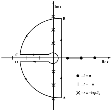
Figure 1: The contour integral on the complex $t$-plane for the strong degeneracy. The poles at $t=n$, $t=-n$, and $t=\pm(i\pi p)/l_{o}$, $p=1,2,\cdots$ are shown with different notations.

when $B\rightarrow 0$. Since electron just has a tiny mass, the electron gas is in general strong degeneracy. So we will stop here for the case of weak degeneracy. For the case of strong degeneracy, i.e. $(\beta\tau-2\varsigma l_{o})>0$, one adopt a closed contour along the left complex plane as shown in Fig. 1. The residues arising from poles $t=\pm(i\pi p)/l_{o}$, $p=1,2,\cdots$, are given by

$$R_{\pm p}=-\frac{(-1)^{p}\sqrt{l_{o}}\cosh\left(\frac{l_{s}}{l_{o}}\pi p\right)}{(\pi p)^{3/2}\sinh\left(\frac{\pi^{2}p}{l_{o}}\right)}e^{\pm i\pi\left(\frac{\beta\tau p}{l_{o}}-2\varsigma p-\frac{1}{4}\right)}.$$ (25)

The contour integral can then be written as

$$\oint=\int_{A}^{B}+\int_{BC}+\int_{DA}+\int_{\gamma}=2\pi i\sum_{p=1}^{\infty}\left(R_{+p}+R_{-p}\right),$$ (26)

where $\gamma$ indicates that the range of the integration is along the branch cut from $C$ to $D$. Since $(\beta\tau-2\varsigma l_{o})>0$, the integrals $\int_{BC}$ and $\int_{DA}$ vanish as the radius $r\rightarrow\infty$. The grand partition function becomes

$$\ln{\cal Z}=-\frac{Vl_{o}}{i\lambda^{3}}\int_{\gamma}\frac{\cosh(l_{s}t)e^{(\beta\tau-2\varsigma l_{o})t}}{t^{3/2}\sin(\pi t)\sinh(l_{o}t)}dt$$

$$-\frac{4Vl_{o}^{3/2}}{\lambda^{3}\sqrt{\pi}}\sum_{p=1}^{\infty}\frac{(-1)^{p}\cos\left(\frac{l_{s}}{l_{o}}\pi p\right)}{(p)^{3/2}\sinh\left(\frac{\pi^{2}p}{l_{o}}\right)}\cos\left[\pi\left(\frac{\beta\tau p}{l_{o}}-2\varsigma p-\frac{1}{4}\right)\right].$$ (27)

Again, due to the fact that $(\beta\tau-2\varsigma l_{o})>0$, the dominant contribution of the contour integral $\int_{\gamma}$ is around the neighborhood of $\left|t\right|=0$ such that the integral

$$-\frac{l_{o}}{2i}\int_{\gamma}\frac{\cosh(l_{s}t)e^{(\beta\tau-2\varsigma l_{o})t}}{t^{3/2}\sin(\pi t)\sinh(l_{o}t)}dt$$

$$=-\frac{1}{2\pi i}\int_{\gamma}e^{(\beta\tau-2\varsigma l_{o})t}t^{-7/2}\left[1+\left(\frac{\pi^{2}}{6}+\frac{l_{s}^{2}}{2}-\frac{l_{o}^{2}}{6}\right)t^{2}+O(t^{4})\right]$$

$$=\frac{8}{15\sqrt{\pi}}y^{5/2}\left[1+\frac{5\pi^{2}}{8}y^{-2}+\frac{15}{8}\left(l_{s}^{2}-\frac{l_{o}^{2}}{3}\right)y^{-2}\right].$$ (28)

Here $y\equiv(\beta\tau-2\varsigma l_{o})$, and we have used the representation of Hankel’s contour integral for Gamma function

$$\frac{1}{\Gamma(z)}=-\frac{1}{2\pi i}\int_{\gamma}t^{-z}e^{t}dt.$$ (29)

The grand partition function for the gas of spin-1/2 electrons in magnetic field and flux is finally given by

$$\ln{\cal Z}=\frac{2V}{\lambda^{3}}\frac{8}{15\sqrt{\pi}}y^{5/2}\left[1+\frac{5\pi^{2}}{8}y^{-2}+\frac{15}{8}\left(l_{s}^{2}-\frac{l_{o}^{2}}{3}\right)y^{-2}\right]$$

$$-\frac{4Vl_{o}^{3/2}}{\lambda^{3}\sqrt{\pi}}\sum_{p=1}^{\infty}\frac{(-1)^{p}\cos\left(\frac{l_{s}}{l_{o}}\pi p\right)}{(p)^{3/2}\sinh\left(\frac{\pi^{2}p}{l_{o}}\right)}\cos\left[\pi\left(\frac{\beta\tau p}{l_{o}}-2\varsigma p-\frac{1}{4}\right)\right].$$ (30)

The last term is an oscillatory term which becomes significance when the system is presented in a strong magnetic field ($l_{s}=l_{o}\geq 1$). In the following section, we shall see that the paramagnetism and diamagnetism come from the third term of the first middle bracket that turns into dominant when the system is presented in a weak magnetic field ($l_{s},l_{o}<<1$). The first two terms are the result of a electron gas with strong degeneracy.

III Effects of a Magnetic Flux in Paramagnetism, Diamagnetism,and dHvA Oscillation

We first discuss the conditions of strong degeneracy ($y\gg 1$) and weak magnetic field ($l_{s},l_{o}<<1$). In this case, the oscillatory term can be neglected, and

$$\ln{\cal Z}\approx\frac{2V}{\lambda^{3}}\frac{8}{15\sqrt{\pi}}y^{5/2}\left[1+\frac{5\pi^{2}}{8}y^{-2}\right].$$ (31)

With this approximation, the density of the degenerate electron gas is related to the Fermi energy as follows:

$$n=\frac{1}{V}\frac{\partial}{\partial(\beta\tau)}\ln{\cal Z}=\frac{8}{3\sqrt{\pi}\lambda^{3}}y^{3/2}\left[1+\frac{\pi^{2}}{8}y^{-2}\right]$$

$$\approx\frac{8}{3\sqrt{\pi}\lambda^{3}}(\beta\tau)^{3/2}\left[1+\frac{\pi^{2}}{8}(\beta\tau)^{-2}-\frac{3\varsigma l_{o}}{\beta\tau}+O\left(\frac{l_{o}}{\left(\beta\tau\right)^{3}}\right)\right]$$

$$\equiv\frac{8}{3\sqrt{\pi}\lambda^{3}}(\beta\epsilon_{f})^{3/2}=\frac{8}{3\sqrt{\pi}}\left(\frac{\mu\epsilon_{f}}{2\pi\hbar^{2}}\right)^{3/2},$$ (32)

where $\epsilon_{f}=(3\pi^{2}n\hbar^{3})^{2/3}/2\mu$ is the Fermi energy of electrons at zero temperature $T=0$. Eq. (32) gives the value of $\beta\tau$ in terms of $\beta\epsilon_{f}$

$$\beta\tau\approx\left(\beta\epsilon_{f}+2\varsigma l_{o}\right)\left[1-\frac{\pi^{2}}{12}\left(\beta\epsilon_{f}+2\varsigma l_{o}\right)^{-2}\right].$$ (33)

With this connection, one can connect the flux effects with the magnetisms of electron gas. As usual, the magnetization $M$ and the magnetic susceptibility $\chi$ are expressed as follows:

$$M=\frac{1}{V}\beta^{-1}\frac{\partial}{\partial B}\ln{\cal Z},\quad\chi=\mu_{0}\frac{M}{B}=\frac{\mu_{0}}{\beta V}\frac{\partial}{B\partial B}\ln{\cal Z},$$ (34)

where $\mu_{0}$ is the permeability of the vacuum. With the conditions $y\gg 1$ and $l_{s},l_{o}<<1$, the dominant contribution of (30) comes from the first middle bracket. It follows that

$$\chi=\frac{\mu_{0}}{\beta B}\frac{16}{15\sqrt{\pi}\lambda^{3}}\left\{\frac{5}{2}y^{3/2}(-2\varsigma\beta\mu_{B})+\frac{5\pi^{2}}{8}y^{-1/2}(-\varsigma\beta\mu_{B})\right.$$

$$+\left.\frac{15}{8}\left(l_{s}^{2}-\frac{1}{3}l_{o}^{2}\right)\left[\frac{2}{B}y^{1/2}-\varsigma\beta\mu_{B}y^{-1/2}\right]\right\},$$ (35)

where the main contributions come from the terms including $y^{1/2}$ and $y^{3/2}$. With the help of (33), the term with variable $y^{1/2}$ can be identified with the well-known Pauli paramagnetism

$$\chi_{{\rm P}}=\frac{3\mu_{0}}{2}\frac{n\mu_{B}^{2}}{\epsilon_{f}}\left[1-\frac{\pi^{2}}{24}\left(\frac{kT}{\epsilon_{f}}\right)^{2}+O\left(\frac{l_{o}}{\beta\epsilon_{f}}\right)^{2}\right],$$ (36)

and the Landau diamagnetism

$$\chi_{{\rm L}}=-\frac{\mu_{0}}{2}\frac{n\mu_{B}^{2}}{\epsilon_{f}}\left[1-\frac{\pi^{2}}{24}\left(\frac{kT}{\epsilon_{f}}\right)^{2}+O\left(\frac{l_{o}}{\beta\epsilon_{f}}\right)^{2}\right].$$ (37)

The contribution of the term including $y^{3/2}$ gives

$$\chi_{{\rm AB}}=-\varsigma\frac{2n\mu_{0}\mu_{B}^{2}}{\mu_{B}B}\left[1-\frac{\pi^{2}}{8}\left(\frac{kT}{\epsilon_{f}}\right)^{2}\right],$$ (38)

which is an effect of diamagnetism. The subscript AB indicates the contribution comes from the magnetic flux of Aharonov-Bohm. Under the general condition, $\mu_{B}B\ll kT\ll\epsilon_{f}$, $\chi_{{\rm AB}}$ may become more important than the Landau diamagnetism $\chi_{{\rm L}}$ when the value of the nonquantized flux $\varsigma\rightarrow 1$. However, it will vanish if $\varsigma\rightarrow 0$. We see the nonlocal effect of flux in the statistical magnetism of an electron gas is significant, and depends on the nonquantized value of the flux. On the other hand, the paramagnetism does not affected by the flux which is reasonable since the flux does affect the space degree of freedom, not the internal degree of freedom.

In the condition of an strong magnetic field, $\mu_{B}B\approx kT\ll\epsilon_{f}$, the oscillatory part

$$\left(\ln{\cal Z}\right)_{{\rm osc}}=-\frac{4Vl_{o}^{3/2}}{\lambda^{3}\sqrt{\pi}}\sum_{p=1}^{\infty}\frac{\cos\left[\pi\left(\frac{\beta\tau p}{l_{o}}-2\varsigma p-\frac{1}{4}\right)\right]}{(p)^{3/2}\sinh\left(\frac{\pi^{2}p}{l_{o}}\right)}$$ (39)

becomes important, where $l_{o}=l_{s}$ is considered. The dominant contribution to the susceptibility is the cosine function. So the susceptibility reads

$$(\chi)_{{\rm osc}}=\frac{\mu_{0}}{\beta V}\frac{\partial}{B\partial B}\left(\ln{\cal Z}\right)_{{\rm osc}}$$

$$\approx-\frac{\mu_{0}\sqrt{2\mu_{B}}\mu^{3/2}kT}{\pi\hbar^{3}B^{3/2}}\left(\epsilon_{f}+2\varsigma\mu_{B}B\right)$$

$$\times\sum_{p=1}^{\infty}\frac{\sin\left[\pi\left(\frac{p\epsilon_{f}}{\mu_{B}B}-\frac{1}{4}\right)\right]}{(p)^{1/2}\sinh\left(\frac{\pi^{2}pkT}{\mu_{B}B}\right)},$$ (40)

where we have used (33) to approximate the $\beta\tau$ and omits the small quantity $-\pi p(kT)^{2}/(12\mu_{B}B\epsilon_{f})$ in the sine function. The second term in the former factor is the effect of the flux which linearly increases the amplitude of the dHvA oscillation. In fact, we can show that when $\varsigma\rightarrow 1$ the flux effect is more important than contributions from $l_{o}^{3/2}$ and $\left[\sinh\left(\pi^{2}p/l_{o}\right)\right]^{-1}$ in (39). Indeed, the differentiation $\partial/\partial B$ with respect to $l_{o}^{3/2}$ and $\left[\sinh\left(\pi^{2}p/l_{o}\right)\right]^{-1}$ in (39) give the contributions

$$-\frac{3\mu_{0}\sqrt{2\mu_{B}}\mu^{3/2}kT}{2\pi^{2}\hbar^{3}B^{3/2}}\mu_{B}B$$

$$\times\sum_{p=1}^{\infty}\frac{\cos\left[\pi\left(\frac{\beta\tau p}{l_{o}}-2\varsigma p-\frac{1}{4}\right)\right]}{(p)^{3/2}\sinh\left(\frac{\pi^{2}p}{l_{o}}\right)},$$ (41)

and

$$-\frac{\mu_{0}\sqrt{2\mu_{B}}\mu^{3/2}(kT)^{2}}{\hbar^{3}B^{3/2}}$$

$$\times\sum_{p=1}^{\infty}\frac{\cos\left[\pi\left(\frac{\beta\tau p}{l_{o}}-2\varsigma p-\frac{1}{4}\right)\right]\cosh\left(\frac{\pi^{2}p}{l_{o}}\right)}{p^{1/2}\sinh^{2}\left(\frac{\pi^{2}p}{l_{o}}\right)}.$$ (42)

Both are smaller than the second term in (40) when $\varsigma\rightarrow 1$. Before finalizing the paper, let us compare the magnitude of magnetization between the oscillatory part and nonoscillatory part. The magnetization of the later is given by

$$M=\frac{B}{\mu_{0}}\chi=\frac{B}{\mu_{0}}(\chi_{{\rm P}}+\chi_{{\rm L}}+\chi_{{\rm AB}})$$

$$\sim\left(\sqrt{\epsilon_{f}}-\epsilon_{f}^{3/2}\frac{\varsigma}{\mu_{B}B}\right)B\mu^{3/2}\mu_{B}^{2}\hbar^{-3}.$$ (43)

The oscillatory part approximates to

$$M_{{\rm osc}}=\frac{B}{\mu_{0}}\chi_{{\rm osc}}$$

$$\sim\left(\epsilon_{f}+2\varsigma\mu_{B}B\right)B^{1/2}\mu^{3/2}\mu_{B}^{3/2}\hbar^{-3}.$$ (44)

The ratio between these two parts has the order of magnitude

$$\frac{M_{{\rm osc}}}{M}\sim\frac{1}{\sqrt{\epsilon_{f}\mu_{B}B}}\left[\frac{1+\frac{2\varsigma\mu_{B}B}{\epsilon_{f}}}{\frac{1}{\epsilon_{f}}-\frac{\varsigma}{\mu_{B}B}}\right].$$ (45)

When $B=10$ Tesla, the quantity $\mu_{B}B\sim 5.8\times 10^{-4}$ eV. The Fermi energy $\epsilon_{f}$ of the electron gas in metals is of the order of a few electron volts. The ratio $M_{{\rm osc}}/M$ is a significant quantity when the value of fractional magnetic flux $\zeta\rightarrow 0$. In this case the oscillatory part dominates the magnetization. On the other side $\varsigma\rightarrow 1$, nonoscillatory part $M$ would be dominant the magnetization.

IV Conclusions

In this paper, the effects of a magnetic flux in statistical magnetisms, including Pauli paramagnetism, Landau diamagnetism, and the dHvA oscillation, of a degenerate electron gas in a magnetic field of arbitrary strength are studied. It is shown that the diamagnetism can be increased by the fractional magnetic flux, and the amplitude of the magnetic oscillation of dHvA can be amplified by the quantum effect of the flux. Since the effect of vortex in a degenerate Fermi gas can be realized in the experiment nowadays 13 and is important in exploring the critical states of matter, the result may be useful in studying the statistical properties of a degenerate Fermi gas involving the vortex.

ACKNOWLEDGMENTS

The author would like to thank Prof. Jang-Yu Hsu for critical reading the paper, and Dr. Jun-Bin Wu for plotting the figure. This work is supported by National Science Council of Taiwan.

References

- (1) S. Nakajima, Y. Murayama, and A. Tonomura (editors), Fundations of Quantum Mechanics in the Light of New Technology, World Scientific, Singapore (1996).
- (2) L. D. Landau, Z. Phys. 64 (1930), 629-637.
- (3) L. D. Landau, and E. M. Lifshitz, Statistical Physics, Part 1, Pergamon, Oxford (1980); p. 171.
- (4) W. J. de Haas, and P. M. van Alphen, Proc. Acad. Amsterdam 33 (1930), 680-690.
- (5) D. Shoenberg, Magnetic Oscillations in Metals, Cambridge University Press, England (1984).
- (6) A. K. Geim, S. V. Dubonos, I. V. Grigorieva, K. S. Novoselov, F. M. Peeters, and V. A. Schweigert, Nature 407 (2000), 55-57; A. K. Geim, S. V. Dubonos, J. J. Palacios, I. V. Grigorieva, M. Henini, and J. J. Schermer, Phys. Rev. Lett. 85 (2000), 1528-1531.
- (7) P. A. M. Dirac, Proc. Roy. Soc., Ser. A 133 (1931), 60-72.
- (8) C. N. Yang, Phys. Rev. Lett. 33 (1974), 445-447.
- (9) R. Jackiw, Phys. Rev. Lett. 50 (1983), 555-559; Phys. Rev. D 29 (1984), 2375-2377.
- (10) H. Kleinert, Path Integrals in Quantum Mechanics, Statistics, and Polymer Physics, 2nd edition, World Scientific, Singapore (1995).
- (11) W. T. Grandy, Jr., Foundations of Statistical Mechanics, Vol. I, Reidel (1987); Ch. 6.
- (12) H. W. Peng, and X. S. Xu, The Fundamentals of Theoretical Physics, Peking University Press, Beijing (1999); Ch. 13.
- (13) M. W. Zwierlein, J. R. Abo-Shaeer, A. Schirotzek, C. H. Schunck, and W. Ketterle, Nature 435 (2005), 1047-1051.