Effect of antiferromagnetic exchange interactions on the Glauber dynamics of one-dimensional Ising models

Abstract

We study the effect of antiferromagnetic interactions on the single spin-flip Glauber dynamics of two different one-dimensional (1D) Ising models with spin $\pm 1$. The first model is an Ising chain with antiferromagnetic exchange interaction limited to nearest neighbors and subject to an oscillating magnetic field. The system of master equations describing the time evolution of sublattice magnetizations can easily be solved within a linear field approximation and a long time limit. Resonant behavior of the magnetization as a function of temperature (stochastic resonance) is found, at low frequency, only when spins on opposite sublattices are uncompensated owing to different gyromagnetic factors (i.e., in the presence of a ferrimagnetic short range order). The second model is the axial next-nearest neighbor Ising (ANNNI) chain, where an antiferromagnetic exchange between next-nearest neighbors (nnn) is assumed to compete with a nearest-neighbor (nn) exchange interaction of either sign. The long time response of the model to a weak, oscillating magnetic field is investigated in the framework of a decoupling approximation for three-spin correlation functions, which is required to close the system of master equations. The calculation, within such an approximate theoretical scheme, of the dynamic critical exponent $z$, defined as ${1/\tau}\approx({1/{\xi}})^{z}$ (where $\tau$ is the longest relaxation time and $\xi$ is the correlation length of the chain), suggests that the $T=0$ single spin-flip Glauber dynamics of the ANNNI chain is in a different universality class than that of the unfrustrated Ising chain.

I Introduction

After the publication of fundamental papersParisi ; Gammaitoni on stochastic resonance (SR), it was realized that the response amplitude of a nonlinear dynamic system to an external periodic signal is greatly enhanced as a function of noise strength, in the presence of a matching between the frequency of the external force and the escape rate across an intrinsic energy barrier. Most of the SR researchreviewSR was pursued on dynamic systems with a double well potential, subject to both periodic and random forces, while only a few investigations of SR in extended or coupled systems have yet been conducted.Sievert

The Ising model with Glauber dynamicsGlauber can be viewed as a set of coupled two-state oscillators, where the coherent signal is provided by an external oscillating magnetic field and thermal fluctuations are the only source of random noise. Each spin is assumed to be in interaction with a heat reservoir of some sort, which causes it to flip between the values $\sigma=+1$ and $\sigma=-1$ randomly with time. In the presence of magnetic coupling between the spins, the transition probability for one spin to flip is assumed to depend on the configuration of the neighboring spins. The time evolution of the system is described by a master equation where the transition rates verify the detailed-balance condition. Solving the master equation, the time dependence of the magnetization and of the spin correlation functions can be obtained. For exchange interaction limited to nearest neighbor (nn) spins, the response of the Ising model with Glauber dynamics to an oscillating magnetic field was investigated in one (1D),Glauber ; Brey_Prados two (2D),Neda2D and three (3D)Neda3D ; Neda23D spatial dimensions. For the 1D nn Ising ferromagnet, Brey and PradosBrey_Prados obtained an analytic expression, within the linear field approximation, for the amplitude and the phase of the induced magnetization. The amplitude always presents a maximum as a function of temperature, with a genuine resonant behavior only for low frequencies. The Glauber dynamics of the 1D Ising model with antiferromagnetic next-nearest neighbor (nnn) exchange interaction competing with the nn one was investigated by Yang,Yang who employed a decoupling approximation to solve the master equation and get an analytical expression for the time-dependent magnetization. He also found, by heuristic arguments, the dynamic critical exponent $z$, defined as ${1/\tau}\approx({1/\xi})^{z}$ (where $\tau$ is the longest relaxation time and $\xi$ is the correlation length of the chain)daSilva , to be $z=2$, the same as that of the unfrustrated 1D nn Ising model.

In this paper, we study - at finite temperature $T>0$ - the effect of antiferromagnetic (AF) exchange interactions on the single spin-flip Glauber dynamics of two different one-dimensional Ising models. Our interest in kinetic 1D Ising models with AF interactions is motivated by recently sinthesized cobalt-basedCaneschi ; Vindigni and rare-earth-basedBogani ; Bernot single chain magnets, showing slow relaxation of the magnetization at low temperature. The magnetic properties of the former chain compound, [Co(hfac)₂NITPhOMe], can be described in terms of a 1D Ising model with AF nn exchange coupling.Vindigni ; Regnault However, the resulting short range order is ferrimagnetic, owing to the alternation along the chain of two different kinds of magnetic centers (a metal ion, Co²⁺, and a nitronyl-nitroxide radical, PhOMe), both with $S=1/2$ but with different gyromagnetic factors. In spite of further complications due to non-collinearity of the spins,Regnault this system was shown to be the first experimental realization of a 1D nn Ising model with Glauber dynamics.Vindigni The single chain magnets belonging to the latter class of rare-earth-based compounds, of general formula [M(hfac)₃(NiTPhOPh)], where M=Eu, Gd, Tb, Dy, Ho, Er, or Yb, and PhOPh is a nitronyl-nitroxide radical, are characterized by strong Ising-type anisotropy and by the simultaneous presence of both nn and nnn exchange interactions between the magnetic centers, with the last ones being antiferromagnetic in nature.Bogani ; Bernot

The paper is organized as follows. In Section II we investigate the Glauber dynamics in a collinear Ising chain, with antiferromagnetic exchange interaction limited to nearest neighbors and different gyromagnetic factors on the two opposite sublattices, subject to an oscillating magnetic field. The system of master equations describing the time evolution of sublattice magnetizations can easily be solved within a linear field approximation and a long time limit. Resonant behavior of the magnetization as a function of temperature (stochastic resonance) is found, at low frequency, only when spins on opposite sublattices are uncompensated owing to different gyromagnetic factors (i.e., in the presence of a ferrimagnetic short range order). In Section III we investigate the 1D axial next-nearest neighbor Ising (ANNNI) model, where an antiferromagnetic exchange between next-nearest neighbor spins is assumed to compete with a nearest-neighbor exchange interaction of either sign. The long time response of the model to a weak, oscillating magnetic field is investigated in the framework of a decoupling approximation (required in order to close the system of master equations) for three-spin correlation functions, which in principle is more accurate than the one reported in Ref. Yang, . As a consequence, our approximate calculation of the dynamic critical exponent $z$ suggests that the $T=0$ single spin-flip Glauber dynamics of the ANNNI chain is in a different universality class than that of the unfrustrated Ising chain. Finally, the conclusions are drawn in Section IV.

II Glauber dynamics in the nearest-neighbor ferrimagnetic Ising chain

We consider a one-dimensional Ising model with a nearest-neighbor antiferromagnetic exchange interaction, $J<0$, in the presence of a time-dependent external field. The Hamiltonian of the system is

$${\cal H}=-J\sum_{j=1}^{N}\sigma^{z}_{j}\sigma^{z}_{j+1}-\mu_{0}~{}H(t)\sum_{j=1}^{N/2}(g_{A}~{}\sigma^{z}_{2j-1}+g_{B}~{}\sigma^{z}_{2j})$$ (1)

where $\mu_{0}$ is the Bohr magneton, and $H(t)=H_{0}e^{-i\omega t}$ is an external magnetic field applied along the $z$ direction and oscillating in time with frequency $\omega$. Spins on opposite sublattices are allowed to take possibly different gyromagnetic factors ($g_{A}\neq g_{B}$), while we assume $\sigma^{z}_{j}=\pm 1$ $\forall j$. Hereafter, the $z$ index will be dropped for ease of notation. In the absence of a magnetic field, if $g_{A}\neq g_{B}$ the ground state is ferrimagnetic, with opposite uncompensated magnetizations on the two sublattices; if $g_{A}=g_{B}$ the ground state is antiferromagnetic, with compensated sublattice magnetizations.

When the system is endowed with single spin-flip Glauber dynamics,Glauber its time evolution is described by the master equation

$${{\partial}\over{\partial t}}p(\sigma,t)=\sum_{j}\Big{[}W_{j}(R_{j}\sigma)p(R_{j}\sigma,t)-W_{j}(\sigma)p(\sigma,t)\Big{]}$$ (2)

where $p(\sigma,t)$ is the probability for the system to assume the configuration $\sigma=\{\sigma_{1},\cdots,\sigma_{j},\cdots,\sigma_{N}\}$ at time $t$, $R_{j}\sigma$ is the configuration obtained from $\sigma$ by flipping spin $j$, and $W_{j}(\sigma)$, $W_{j}(R_{j}\sigma)$ are the transition rates between such configurations.

For a 1D Ising model of spins ($\sigma_{j}=\pm 1$) with ferromagnetic nn exchange interaction $J>0$ and gyromagnetic factor $g$, Brey and PradosBrey_Prados showed that, for low frequency, a stochastic resonance phenomenon occurs: i.e., the induced magnetization $M(t)=g\mu_{0}\sum_{j=1}^{N}\langle\sigma_{j};t\rangle$ oscillates at the same frequency as the magnetic field, and the amplitude of $M(t)$ presents a sharp maximum as a function of temperature $T$. The resonance temperature, $T_{\rm r}$, is determined by the matching between the frequency, $\omega$, of the external field and the inverse of the statistical time scale, $1/\tau(T_{\rm r})$, associated to the spontaneous (i.e., in zero field) decay of the magnetization. In zero field, the magnetization of the 1D nn Ising ferromagnet was foundGlauber ; Brey_Prados to relax to its equilibrium value, $M=0$, with the asymptotic $t\to\infty$ behavior $M(t)\approx e^{-t/\tau(T)}/\sqrt{t}$. The relaxation time $\tau$ was found to be exponentially divergent for $T\to 0$, $\tau(T)\approx e^{{4J}\over{kT}}$ (where $k$ denotes Boltzmann’s constant), and to become of the order of the inverse of the transition rate of an isolated spin for $T\to\infty$, $\tau\approx 1/\alpha$.Glauber ; Brey_Prados

For a 1D Ising model with antiferromagnetic nn exchange interaction ($J<0$), the master equation (2) is still the starting point for the study of the chain dynamics. In this case, if $g_{A}\neq g_{B}$, the transition rates in the presence of a field are assumed to be different for even ($A$) and odd ($B$) lattice sites $j$

$$W_{j}(\sigma)=W_{j}^{(0)}(\sigma)\Big{[}1-\sigma_{j}\tanh(\beta_{A,B})\Big{]}={1\over 2}\alpha~{}\Big{[}1-{1\over 2}\gamma\sigma_{j}(\sigma_{j-1}+\sigma_{j+1})\Big{]}~{}\Big{[}1-\sigma_{j}\tanh(\beta_{A,B})\Big{]}$$ (3)

where $W_{j}^{(0)}(\sigma)$ denote the transition rates in zero field. The transition rate of an isolated spin, ${1\over 2}\alpha$, is considered as temperature independent and sets the time scale. In the case of interacting spins, the probability per unit time of the $j$-th spin to flip depends on the orientation of its nearest neighbors. The magnetic field favors one orientation with respect to the other. A correspondence between the parameters $\gamma$, $\beta_{A,B}$ of the stochastic model and the parameters $J$, $g_{A,B}\mu_{0}H(t)$ of the statistical Ising model can be obtainedGlauber ; Brey_Prados observing that at equilibrium ${{\partial}\over{\partial t}}p(\sigma,t)=0$, so that

$$\sum_{j}\Big{[}W_{j}(R_{j}\sigma)p_{eq}(R_{j}\sigma,t)\Big{]}=\sum_{j}\Big{[}W_{j}(\sigma)p_{eq}(\sigma,t)\Big{]}.$$ (4)

Next, requiring the detailed balance (i.e., the microscopic reversibility) condition to be satisfied

$${{W_{j}(R_{j}\sigma)}\over{W_{j}(\sigma)}}={{p_{eq}(\sigma,t)}\over{p_{eq}(R_{j}\sigma,t)}},$$ (5)

with $p_{eq}(\sigma,t)=e^{-{{{\cal H}(\sigma)}\over{kT}}}$ and $p_{eq}(R_{j}\sigma,t)=e^{-{{{\cal H}(R_{j}\sigma)}\over{kT}}},$ one readily obtains

$$\gamma=\tanh\Big{(}{{2J}\over{kT}}\Big{)},~{}~{}~{}\beta_{A,B}=\tanh\Big{(}{{g_{A,B}\mu_{0}H(t)}\over{kT}}\Big{)}.$$ (6)

The evolution equation for the spin expectation value $\langle\sigma_{j};t\rangle=\sum_{\sigma}\sigma_{j}p(\sigma,t)$ is directly obtained from the master equation to be ${{\partial}\over{\partial t}}\langle\sigma_{j};t\rangle=-2\langle\sigma_{j}W_{j}(\sigma);t\rangle$.Glauber ; Brey_Prados Considering that for model (1) the spins belong to two opposite sublattices, the system of evolution equations in the presence of an oscillating field is

$${{\partial}\over{\partial(\alpha t)}}\langle\sigma_{2j-1};t\rangle = -\langle\sigma_{2j-1};t\rangle+{1\over 2}\gamma\Big{(}\langle\sigma_{2j-2};t\rangle+\langle\sigma_{2j};t\rangle\Big{)}+\beta_{A}\Big{[}1-{1\over 2}\gamma\Big{(}\langle\sigma_{2j-2}\sigma_{2j-1};t\rangle+\langle\sigma_{2j-1}\sigma_{2j};t\rangle\Big{)}\Big{]}$$ (7)

$${{\partial}\over{\partial(\alpha t)}}\langle\sigma_{2j};t\rangle = -\langle\sigma_{2j};t\rangle+{1\over 2}\gamma\Big{(}\langle\sigma_{2j-1};t\rangle+\langle\sigma_{2j+1};t\rangle\Big{)}+\beta_{B}\Big{[}1-{1\over 2}\gamma\Big{(}\langle\sigma_{2j-1}\sigma_{2j};t\rangle+\langle\sigma_{2j}\sigma_{2j+1};t\rangle\Big{)}\Big{]}$$ (8)

The system is not closed owing to the presence of two-spin, time-dependent correlation functions on the right hand sides. In order to solve it, a linear field approximation is madeGlauber ; Brey_Prados so that $\tanh[(g_{A,B}\mu_{0}H_{0})/(kT)]$ can be expanded for small values of the argument and two-spin correlations can be evaluated in the absence of a field. Moreover, if in the long time limit $t\to\infty$ the nn correlation functions are assumedGlauber ; Brey_Prados to take their equilibrium value $\langle\sigma_{j}\sigma_{j+1};t\rangle\to\eta=\tanh[J/(kT)]$, the system of two coupled equations of motion for the two sublattice magnetizations

$$M_{1}(t)=g_{A}\mu_{0}\sum_{j=1}^{N/2}\langle\sigma_{2j-1};t\rangle,~{}~{}~{}M_{2}(t)=g_{B}\mu_{0}\sum_{j=1}^{N/2}\langle\sigma_{2j};t\rangle$$ (9)

can be written in matrix form

$$\left(\begin{array}[]{c}{{\partial}\over{\partial(\alpha t)}}M_{1}(t)\\ {{\partial}\over{\partial(\alpha t)}}M_{2}(t)\end{array}\right)+\left(\begin{array}[]{cc}1&-{{g_{A}}\over{g_{B}}}\gamma\\ -{{g_{B}}\over{g_{A}}}\gamma&1\end{array}\right)\left(\begin{array}[]{c}M_{1}(t)\\ M_{2}(t)\end{array}\right)={\cal N}(T)\left(\begin{array}[]{c}g_{A}^{2}\\ g_{B}^{2}\end{array}\right)e^{-i\omega t}$$

(10)

Taking into account that $\gamma={{2\eta}\over{1+\eta^{2}}}$, the temperature dependent coefficient ${\cal N}(T)$ can be expressed as

$${\cal N}(T)={N\over 2}{{\mu_{0}^{2}H_{0}}\over{kT}}(1-\gamma\eta)={N\over 2}{{\mu_{0}^{2}H_{0}}\over{kT}}{{1-\eta^{2}}\over{1+\eta^{2}}}.$$ (11)

The above system can be decoupled diagonalizing the $2\times 2$ non-symmetric matrix on the l.h.s. of Eq. (10). Denoting by ${\cal M}_{1}(t)$ and ${\cal M}_{2}(t)$ the normal modes, one obtains

$$\left(\begin{array}[]{c}{{\partial}\over{\partial(\alpha t)}}{\cal M}_{1}(t)\\ {{\partial}\over{\partial(\alpha t)}}{\cal M}_{2}(t)\end{array}\right)+\left(\begin{array}[]{cc}\lambda_{1}&0\\ 0&\lambda_{2}\end{array}\right)\left(\begin{array}[]{c}{\cal M}_{1}(t)\\ {\cal M}_{2}(t)\end{array}\right)={\cal N}(T)\left(\begin{array}[]{c}f_{1}\\ f_{2}\end{array}\right)e^{-i\omega t}$$

where the eigenvalues $\lambda_{n}$ ($n=1,2$) turn out to be independent of the gyromagnetic factors $g_{A}$ and $g_{B}$

$$\lambda_{1}=1-\gamma,~{}~{}~{}~{}\lambda_{2}=1+\gamma,$$ (12)

and the $f_{n}$ ($n=1,2$) coefficients are

$$f_{1}={{g_{B}}\over 2}(g_{B}+g_{A})~{}~{}~{}~{}f_{2}={{g_{B}}\over 2}(g_{B}-g_{A}).$$ (13)

The relationships between the normal modes ${\cal M}_{n}(t)$ and the sublattice magnetizations $M_{n}(t)$ ($n=1,2$) are

$${\cal M}_{1}(t)={1\over 2}\Big{[}M_{2}(t)+{{g_{B}}\over{g_{A}}}M_{1}(t)\Big{]},~{}~{}~{}{\cal M}_{2}(t)={1\over 2}\Big{[}M_{2}(t)-{{g_{B}}\over{g_{A}}}M_{1}(t)\Big{]}$$ (14)

(i.e., ${\cal M}_{1}(t)$ and ${\cal M}_{2}(t)$ are related to the net and the staggered magnetization, respectively). Conversely, one has

$$M_{1}(t)={{g_{A}}\over{g_{B}}}\Big{[}{\cal M}_{1}(t)-{\cal M}_{2}(t)\Big{]},~{}~{}~{}M_{2}(t)={\cal M}_{1}(t)+{\cal M}_{2}(t).$$ (15)

The general solution for the normal modes is ($n=1,2$)

$${\cal M}_{n}(t)={\cal M}_{n}(t_{0})e^{-{{t-t_{0}}\over{\tau_{n}}}}+{\cal N}(T)f_{n}\int_{t_{0}}^{t}dt^{\prime}e^{{{t^{\prime}-t}\over{\tau_{n}}}}e^{-i\omega t^{\prime}}$$ (16)

where the relaxation times $\tau_{n}$ are expressed, in terms of the eigenvalues $\lambda_{n}$ of the non-symmetric $2\times 2$ matrix, as $\tau_{n}=1/(\alpha\lambda_{n})$, so that

$$\tau_{1}={1\over{\alpha(1-\gamma)}},~{}~{}~{}\tau_{2}={1\over{\alpha(1+\gamma)}}.$$ (17)

In the absence of an external magnetic field, ${\cal N}(T)=0$, the normal modes ${\cal M}_{n}(t)$ are found to relax exponentially. In the low temperature limit, $T\to 0$, one has $\gamma=\tanh\Big{(}{{2J}\over{kT}}\Big{)}\approx{{J}\over{|J|}}\Big{(}1-2e^{-{{4|J|}\over{kT}}}\Big{)}$, so that for antiferromagnetic nn exchange ($J<0$), the first relaxation time is simply $\tau_{1}\approx{1\over{2\alpha}}$, while the second relaxation time is exponentially diverging with decreasing $T$, $\tau_{2}\approx{1\over{2\alpha}}e^{{{4|J|}\over{kT}}}$. For high temperatures, $kT\gg|J|$, both relaxation times become of the order of the inverse of the transition rate of an isolated spin, $\tau_{1}\approx\tau_{2}\approx 1/\alpha$.

For non vanishing magnetic field, the time dependence of the normal modes is obtained letting $t_{0}\to-\infty$ in Eq. (16)

$${\cal M}_{n}(t)={\cal N}(T){{f_{n}}\over{\lambda_{n}}}{{1}\over{1-i\omega\tau_{n}}}e^{-i\omega t}~{}~{}~{}~{}(n=1,2)$$ (18)

The total magnetization is

$$M_{tot}(t)=M_{1}(t)+M_{2}(t)={{g_{B}+g_{A}}\over{g_{B}}}{\cal M}_{1}(t)+{{g_{B}-g_{A}}\over{g_{B}}}{\cal M}_{2}(t)=\chi(\omega,T)H_{0}e^{-i\omega t},$$ (19)

where the complex susceptibility $\chi(\omega,T)$ is given by

$$\chi(\omega,T)=N~{}{{\mu_{0}^{2}}\over{kT}}~{}\Bigg{[}\Big{(}{{g_{B}+g_{A}}\over 2}\Big{)}^{2}~{}{{1+\eta}\over{1-\eta}}~{}{{1}\over{1-i\omega\tau_{1}}}+\Big{(}{{g_{B}-g_{A}}\over 2}\Big{)}^{2}~{}{{1-\eta}\over{1+\eta}}~{}{{1}\over{1-i\omega\tau_{2}}}\Bigg{]}.$$ (20)

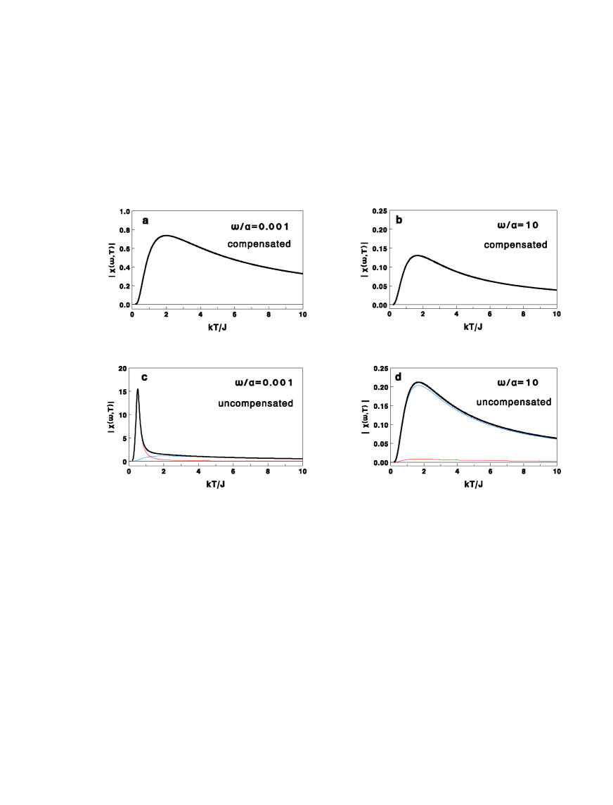
Figure 1: (color online) Temperature dependence of the amplitude of the complex susceptibility $|\chi(\omega,T)|$ for an Ising chain with antiferromagnetic nearest neighbor interaction $J=-1$, subject to a weak external magnetic field oscillating at frequency $\omega$. Figures (a), (b) refer to the compensated case ($g_{A}=g_{B}=2$), while Figures (c) and (d) to the uncompensated case ($g_{A}=2,~{}g_{B}=3$), for selected values of the frequency ($\omega/\alpha=0.001$ and $10$). In Figs. (c,d) the thin (color) lines represent the contributions to the amplitude of the two terms on the r.h.s. of Eq. (20), while the thick (black) line is their sum. A resonant behavior (similar to the one predicted for the nn Ising ferromagnetic chain endowed with single spin-flip Glauber dynamics)Glauber ; Brey_Prados is observed only in the uncompensated case for low frequency (notice the enhanced vertical scale in Fig. c).

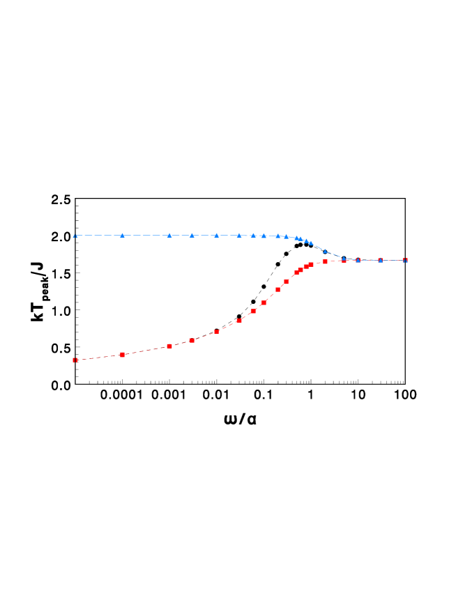
Figure 2: (color online) Frequency dependence of the peak temperature of the amplitude of the complex susceptibility $|\chi(\omega,T)|$ of an Ising chain with nearest neighbor exchange interaction. Triangles: compensated antiferromagnet ($J=-1$, $g_{A}=g_{B}=2$); circles: uncompensated ferrimagnet ($J=-1$, $g_{A}=2$, $g_{B}=3$); squares: ferromagnet ($J=+1$, $g_{A}=g_{B}=2$).Brey_Prados The dashed lines are guides to the eye.

In the limit $\omega\to 0$, the static susceptibility of the Ising ferrimagnetic chain in zero field is correctly recovered: see Appendix A.1, Eq. (79), for details. As regards the dynamic response of the system to a weak, oscillating magnetic field, from Eq. (20) it is apparent that, for antiferromagnetic nn exchange ($J<0$) and $T\to 0$, the first term on the r.h.s. is associated with a fast relaxation, while the second term with an exponentially slow relaxation. Thus, a resonant behavior, similar to the one observed in the ferromagnetic nn Ising chain endowed with single spin-flip Glauber dynamics,Brey_Prados is possible only when spins on opposite sublattices are uncompensated owing to different gyromagnetic factors (i.e., in the presence of ferrimagnetic short range order). See Fig. 1, where the temperature dependence of the amplitude of $\chi(\omega,T)$ is reported, for selected values of the frequency, both in the compensated ($J<0$ and $g_{A}=g_{B}$) and uncompensated ($J<0$ and $g_{A}\neq g_{B}$) case.

The resonant behavior shown by the ferrimagnetic chain at low frequency (see Fig. 1c) is a manifestation of the stochastic resonance phenomenon:reviewSR i.e., the response of a set of coupled bistable systems to a periodic drive is enhanced in the presence of a stochastic noise when a matching occurs between the fluctuation induced switching rate of the system and the forcing frequency. In the ferrimagnetic chain, the role of stochastic noise is played by thermal fluctuations and the resonance peak occurs when the deterministic time scale of the external magnetic field matches with the statistical time scale associated to the spontaneous decay of the net magnetization $M_{tot}(t)$. For low frequency $\omega\ll\alpha$ (i.e., low temperature), the resonance condition for the uncompensated case is

$$\omega^{-1}\approx\tau_{2}(T_{peak}),$$ (21)

while for the compensated case only the mode with fast relaxation $\tau_{1}\approx O(\alpha^{-1})$ contributes, providing a broad peak rather than a genuine resonance. For high frequency $\omega\gg\alpha$ (i.e., high temperature) a broad peak is found, both for the uncompensated and the compensated case, since the two relaxation times $\tau_{1}$ and $\tau_{2}$ become of the order of $1/\alpha$, so that the resonance condition cannot be fulfilled.Brey_Prados

The frequency dependence of the peak temperature $T_{peak}$ is reported in Fig. 2 both for the compensated (antiferromagnetic) and the uncompensated (ferrimagnetic) chain, and compared with the ferromagnetic counterpart.Brey_Prados In the compensated case, the frequency dependence of the peak is very smooth, owing to the smooth temperature dependence of the relaxation time $\tau_{1}$, ranging between $1/(2\alpha)$ at low $T$ and $1/\alpha$ at high $T$. In the uncompensated case, a behavior very similar to the ferromagnetic one is observed for low frequency: the reason is that for low $\omega$ the dominant contribution to $\chi(\omega)$ is provided by the second term on the r.h.s. of Eq. (20). At intermediate frequency, a maximum is observed owing to the coming into play of the first term on the r.h.s. of Eq. (20). Finally, for $\omega\gg\alpha$, the amplitude of $\chi(\omega)$ becomes

$$|\chi(\omega,T)|\approx N~{}{{\mu_{0}^{2}}\over{kT}}~{}{{\alpha}\over{\omega}}~{}\Bigg{[}\Big{(}{{g_{B}+g_{A}}\over 2}\Big{)}^{2}~{}{{1+\eta}\over{1-\eta}}~{}(1-\gamma)+\Big{(}{{g_{B}-g_{A}}\over 2}\Big{)}^{2}~{}{{1-\eta}\over{1+\eta}}~{}(1+\gamma)\Bigg{]}$$ (22)

where both terms in square brackets on the r.h.s. of Eq. (22) present a maximum at the same temperature, which is numerically determined to be $T_{peak}\approx 1.66711|J|$.

III Glauber dynamics in the axial-next-nearest-neighbor-Ising (ANNNI) chain

We consider a 1D axial-next-nearest-neighbor Ising (ANNNI) model with spins alternating on two interlacing sublattices (denoted by $A$ and $B$), with Hamiltonian

$${\cal H}=-J_{1}\sum_{i=1}^{N/2}\Big{(}\sigma^{z}_{2i-1}\sigma^{z}_{2i}+\sigma^{z}_{2i}\sigma^{z}_{2i+1}\Big{)}-J_{2}\sum_{i=1}^{N/2}\Big{(}\sigma^{z}_{2i-1}\sigma^{z}_{2i+1}+\sigma^{z}_{2i}\sigma^{z}_{2i+2}\Big{)}-\mu_{0}H(t)\sum_{i=1}^{N/2}\Big{(}g_{A}\sigma^{z}_{2i-1}+g_{B}\sigma^{z}_{2i}\Big{)}.$$ (23)

The intra-sublattice antiferromagnetic next-nearest neighbor coupling $J_{2}<0$ competes with the inter-sublattice nearest neighbor coupling $J_{1}$, which may be of either sign. In what follows, we shall assume $J_{1}>0$ (ferromagnetic coupling). $H(t)=H_{0}e^{i\omega t}$ is an external magnetic field applied along the $z$ direction and oscillating in time with frequency $\omega$, $\mu_{0}$ denotes the Bohr magneton and the spins $\sigma^{z}_{i}=\pm 1$ are allowed to assume possibly different gyromagnetic factors on odd and even sites ($g_{A}\neq g_{B}$); the $z$ index shall be dropped for ease of notation.

In the limiting case $g_{A}=g_{B}=g$, Eq. (1) reduces to the well-known ANNNI (axial next-nearest-neighbor Ising) model.Selke Depending on the competition ratio $r=-J_{2}/J_{1}$, this model in zero field is known to admit a ferromagnetic ground state for $r<1/2$, and a $(2,2)$ antiphase structure (two spins up, two spins down), with zero magnetization, for $r>1/2$; for $r=1/2$ the ground state is degenerate and disordered.Morita_gs At finite temperatures, the model cannot support long range order; however, a strong short range order is present in the paramagnetic phase. For zero applied field, as far as the thermodynamic properties are concerned,notaYang the 1D ANNNI model can be mapped into an equivalent 1D Ising model with only nearest neigbor interaction in an effective field, and analytic results (see Appendix A.2) can be obtained for the partition function and the spin correlation functions.Stephenson ; Harada In the presence of a static magnetic field, the ground state of the generalized ANNNI model, i.e. a chain of alternating spins with different quantum numbers and different nnn exchange interactions on the two sublattices, was thoroughly investigated,Kim_gs and the thermodynamic properties were exactly calculated (though numerically) by the transfer matrix method.PR_tm ; Kim_tm

Here we aim at investigating the long-time dynamic response of the ANNNI chain, Eq. (23), to a weak, external magnetic field oscillating in time. The time evolution of the system is still described by the master equation (2), but with respect to the case of the nn Ising chain, the transition rates in zero field, $W_{j}^{(0)}(\sigma)$, are now assumed to take the form

$$W_{j}^{(0)}(\sigma)={1\over 2}\alpha\Big{[}1-{1\over 2}\gamma_{1}\sigma_{j}(\sigma_{j-1}+\sigma_{j+1})\Big{]}\Big{[}1-{1\over 2}\gamma_{2}\sigma_{j}(\sigma_{j-2}+\sigma_{j+2})\Big{]}$$ (24)

meaning that the probability per unit time of the $j$-th spin to flip depends on the status of both its nearest neighbors and next nearest neighbors; ${1\over 2}\alpha$, the transition rate of an isolated spin, is arbitrary and sets the time scale. In the presence of a field applied along the $z$ axis, the transition rates $W_{j}(\sigma)$ are given by

$$W_{j}(\sigma)=W_{j}^{(0)}(\sigma)\Big{[}1-\sigma_{j}\tanh(\beta_{A,B})\Big{]}.$$ (25)

As usual, a correspondence between the parameters $\gamma_{1}$, $\gamma_{2}$, $\beta_{A,B}$ of the stochastic model and the parameters $J_{1}$, $J_{2}$, $g_{A,B}\mu_{0}H(t)$ of the statistical ANNNI model can be obtained requiring the detailed balance (i.e., the microscopic reversibility) condition, Eq. (5) to be satisfied at equilibrium. One findsYang

$$\gamma_{1}=\tanh\Big{(}{{2J_{1}}\over{kT}}\Big{)},~{}~{}~{}\gamma_{2}=\tanh\Big{(}{{2J_{2}}\over{kT}}\Big{)},~{}~{}~{}\beta_{A,B}=\tanh\Big{(}{{g_{A,B}\mu_{0}H(t)}\over{kT}}\Big{)}.$$ (26)

The stochastic equation of motion for the spin expectation value $\langle\sigma_{j};t\rangle=\sum_{\sigma}\sigma_{j}p(\sigma,t)$ in the presence of an oscillating field is then obtained, from the master equation, to be ${{\partial}\over{\partial t}}\langle\sigma_{j};t\rangle=-2\langle\sigma_{j}W_{j}(\sigma);t\rangle$, givingYang

$${{\partial}\over{\partial t}}\langle\sigma_{j};t\rangle = -\langle\sigma_{j};t\rangle+{1\over 2}\gamma_{1}\Big{(}\langle\sigma_{j-1};t\rangle+\langle\sigma_{j+1};t\rangle\Big{)}+{1\over 2}\gamma_{2}\Big{(}\langle\sigma_{j-2};t\rangle+\langle\sigma_{j+2};t\rangle\Big{)}$$ (27)

$$- {1\over 4}\gamma_{1}\gamma_{2}\Big{(}\langle\sigma_{j}\sigma_{j-1}\sigma_{j-2};t\rangle+\langle\sigma_{j}\sigma_{j-1}\sigma_{j+2};t\rangle+\langle\sigma_{j}\sigma_{j+1}\sigma_{j-2};t\rangle+\langle\sigma_{j}\sigma_{j+1}\sigma_{j+2};t\rangle\Big{)}$$ (28)

$$+ \tanh\Big{(}{{g_{A,B}\mu_{0}H(t)}\over{kT}}\Big{)}$$ (29)

$$\times \Big{[}1-{1\over 2}\gamma_{1}\Big{(}\langle\sigma_{j}\sigma_{j-1};t\rangle+\langle\sigma_{j}\sigma_{j+1};t\rangle\Big{)}-{1\over 2}\gamma_{2}\Big{(}\langle\sigma_{j}\sigma_{j-2};t\rangle+\langle\sigma_{j}\sigma_{j+2};t\rangle\Big{)}$$ (30)

$$+ {1\over 4}\gamma_{1}\gamma_{2}\Big{(}\langle\sigma_{j-1}\sigma_{j-2};t\rangle+\langle\sigma_{j-1}\sigma_{j+2};t\rangle+\langle\sigma_{j+1}\sigma_{j-2};t\rangle+\langle\sigma_{j+1}\sigma_{j+2};t\rangle\Big{)}\Big{]}.$$ (31)

where we remind that the subscripts $A$ and $B$ refer to the case of $j$ odd and $j$ even, respectively. This set of equations is not closed, owing to the time-dependent two-spin and three-spin correlation functions on the r.h.s. In order to solve it, we make the following approximations.

• For sufficiently weak fields ($x=(g_{A,B}\mu_{0}H_{0})/(kT)\ll 1$), the hyperbolic tangent on the r.h.s. of Eq. (27) is expanded for low values of the argument ($\tanh x\approx x$) and two-spin correlation functions are calculated in the absence of a field.

• Three-spin correlation functions are decoupled, in all possible ways, into products of a single-spin expectation value and a two-spin correlation function

  $$\langle\sigma_{j}\sigma_{j+m}\sigma_{j+n};t\rangle\approx\langle\sigma_{j};t\rangle\langle\sigma_{j+m}\sigma_{j+n};t\rangle+\langle\sigma_{j+m};t\rangle\langle\sigma_{j}\sigma_{j+n};t\rangle+\langle\sigma_{j+n};t\rangle\langle\sigma_{j}\sigma_{j+m};t\rangle.$$ (32)

  Notice that a different, and incomplete, decoupling was adopted in Ref. Yang, , thus leading to different results with respect to the present work.

• For sufficiently long times, two-spin correlation functions between $n$-th neighbors are assumed to be independent of the initial conditions and to take their static equilibrium values $\langle\sigma_{j}\sigma_{j+n};t\rangle\to\eta_{n}$ for $t\to\infty$. Static two-spin correlation functions $\eta_{n}=\langle\sigma_{j}\sigma_{j+n}\rangle$ can be exactly calculated in 1D via the transfer matrix method.Stephenson ; Harada ; PR_tm ; Kim_tm For $g_{A}=g_{B}$ and $H_{0}=0$, analytic resultsStephenson ; Harada can be obtained for $\eta_{n}$: see Appendix A.2 for details.

Under these approximations, the master equation for the spin expectation value on a generic site $j$ becomes

$${{\partial}\over{\partial(\alpha t)}}\langle\sigma_{j};t\rangle = -\Big{[}1+{1\over 2}\gamma_{1}\gamma_{2}(\eta_{1}+\eta_{3})\Big{]}\langle\sigma_{j};t\rangle$$ (33)

$$+ {1\over 2}\gamma_{1}\Big{(}1-\gamma_{2}\eta_{2}\Big{)}\Big{[}\langle\sigma_{j-1};t\rangle+\langle\sigma_{j+1};t\rangle\Big{]}+{1\over 2}\gamma_{2}\Big{(}1-\gamma_{1}\eta_{1}\Big{)}\Big{[}\langle\sigma_{j-2};t\rangle+\langle\sigma_{j+2};t\rangle\Big{]}$$ (34)

$$+ \Big{[}{{g_{A,B}\mu_{0}H(t)}\over{kT}}\Big{]}~{}\Big{[}1-\gamma_{1}\eta_{1}-\gamma_{2}\eta_{2}+{1\over 2}\gamma_{1}\gamma_{2}(\eta_{1}+\eta_{3})\Big{]}.$$ (35)

In the range of the competition ratio $r$ corresponding to weak nnn antiferromagnetism $0<r<{1\over 2}$, the ground state of the model is ferromagnetic (since we have assumed $J_{1}>0$), while for strong nnn antiferromagnetism ${1\over 2}<r<\infty$, the ground state is the so-called $(2,2)$ antiphase state, consisting of two spins up followed by two spins down. The two different regimes shall be investigated separately since they require different order parameters.

III.1 Weak nnn antiferromagnetism (competition ratio $0<r<{1\over 2}$)

In the range of the competition ratio $r$ corresponding to the ferromagnetic ground state ($0<r<{1\over 2}$), owing to the different gyromagnetic factors on odd ($g_{A}$) and even ($g_{B}$) lattice sites, it is necessary to consider the magnetizations over two sublattices, like in Eq. (9), as the order parameter. From the master equation, Eq. (33), one is thus led to consider a system of two coupled equations of motion, which can be written just like Eq. (10), with the elements of the $2\times 2$ non-symmetric matrix now being

$$a_{11} = 1-\gamma_{2}(1-\gamma_{1}\eta_{1})+{1\over 2}\gamma_{1}\gamma_{2}(\eta_{1}+\eta_{3})=a_{22}$$ (36)

$$a_{12} = -{{g_{A}}\over{g_{B}}}\gamma_{1}(1-\gamma_{2}\eta_{2})~{}~{}~{}a_{21}=-{{g_{B}}\over{g_{A}}}\gamma_{1}(1-\gamma_{2}\eta_{2})$$ (37)

and the temperature dependent coefficient

$${\cal N}(T)={N\over 2}{{\mu_{0}^{2}H_{0}}\over{kT}}\Big{[}1-\gamma_{1}\eta_{1}-\gamma_{2}\eta_{2}+{1\over 2}\gamma_{2}\gamma_{1}(\eta_{1}+\eta_{3})\Big{]}.$$ (38)

After diagonalization, the eigenvalues now turn out to be

$$\lambda_{1} = 1-\gamma_{1}(1-\gamma_{2}\eta_{2})-\gamma_{2}(1-\gamma_{1}\eta_{1})+{1\over 2}\gamma_{1}\gamma_{2}(\eta_{1}+\eta_{3})$$ (39)

$$\lambda_{2} = 1+\gamma_{1}(1-\gamma_{2}\eta_{2})-\gamma_{2}(1-\gamma_{1}\eta_{1})+{1\over 2}\gamma_{1}\gamma_{2}(\eta_{1}+\eta_{3}),$$ (40)

independent of the gyromagnetic factors $g_{A}$ and $g_{B}$. The relationships between the normal modes ${\cal M}_{n}(t)$ and the sublattice magnetizations $M_{n}(t)$ ($n=1,2$) are the same as in Eqs. (14), (15). Also the expressions for the $f$-coefficients are the same, i.e. $f_{1}={{g_{B}}\over 2}(g_{B}+g_{A})$, $f_{2}={{g_{B}}\over 2}(g_{B}-g_{A})$. As before, the general solution for the normal modes takes the form in Eq. (16), where the relaxation times are $\tau_{n}={1\over{\alpha\lambda_{n}}}$, with the eigenvalues now given by Eq. (39). Finally, in the case of weak nnn antiferromagnetic coupling, the complex susceptibility of the ANNNI chain turns out to be

$$\chi(\omega,T) = N~{}{{\mu_{0}^{2}}\over{kT}}~{}\Big{[}1-\gamma_{1}\eta_{1}-\gamma_{2}\eta_{2}+{1\over 2}\gamma_{1}\gamma_{2}(\eta_{1}+\eta_{3})\Big{]}$$ (41)

$$\times \Bigg{[}\Big{(}{{g_{B}+g_{A}}\over 2}\Big{)}^{2}{1\over{\lambda_{1}}}{1\over{1-i\omega\tau_{1}}}+\Big{(}{{g_{B}-g_{A}}\over 2}\Big{)}^{2}{1\over{\lambda_{2}}}{1\over{1-i\omega\tau_{2}}}\Bigg{]}.$$ (42)

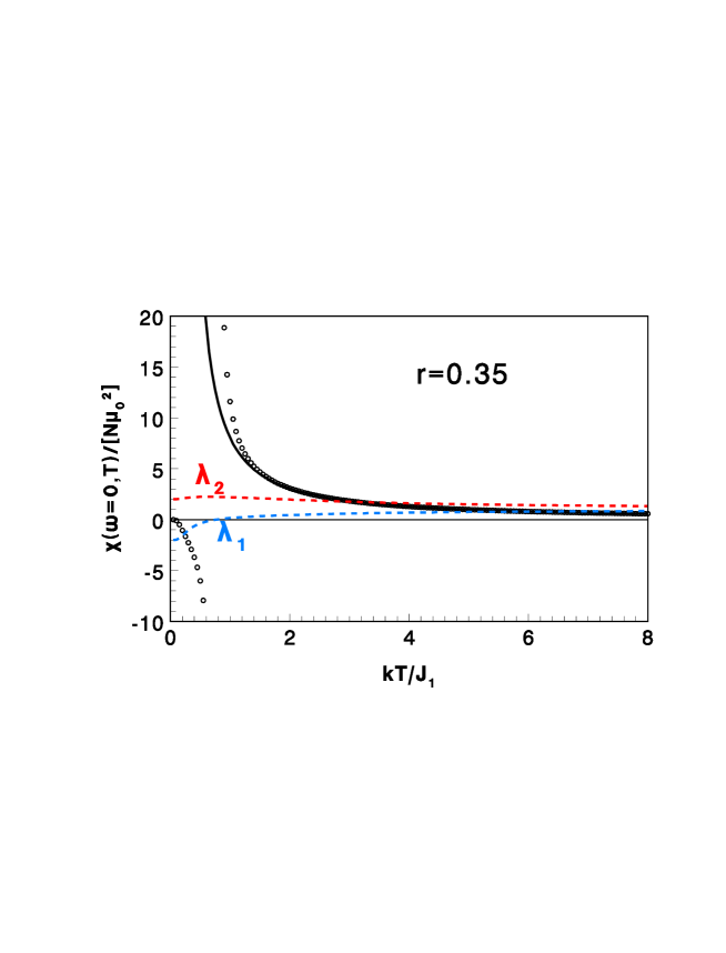
Figure 3: (color online) Temperature dependence of the static susceptibility $\chi(\omega=0,T)$ of an ANNNI chain with $J_{1}=1$, $J_{2}=-0.35$ and $g_{A}=g_{B}=2$, corresponding to a value $r=0.35$ of the competition ratio (weak nnn antiferromagnetism). The thick line is the exact transfer matrix result, while open circles denote the approximate calculation, Eq. (41). The temperature dependence of the eigenvalues $\lambda_{1}$ and $\lambda_{2}$ (39) is also shown by the dashed lines. The approximations made to close the set of master equations (27) are found to fail for low temperatures.

In the limiting case $r=0$, the well-known result for the nn Ising chainGlauber ; Brey_Prados is correctly recovered. In the case $0<r<{1\over 2}$, we show in Fig. 3 that the approximate static susceptibility, calculated from Eq. (41) for zero frequency, turns out to be in good agreement with the exact transfer matrix result,Stephenson ; Harada Eq. (87), only at high temperatures ($kT\gtrsim J_{1}$). In contrast, an unphysical (negative) static susceptibility is obtained at low temperatures, as a consequence of the negative values assumed by the eigenvalue $\lambda_{1}$ for $kT\lesssim J_{1}$.

The low-temperature failure of Eq. (41) can be attributed to the decoupling (32) of three-spin correlation functions, which was made in order to close the set of master equations, Eq. (27): in fact, decoupling approximations have the drawback to be uncontrollable, but in principle they are expected to be more accurate the higher the temperature. Moreover, at low temperatures one can guess another source of error to lie in the assumption that, for sufficiently long times, the spin-spin correlation functions take their static equilibrium values: $\langle\sigma_{j}\sigma_{j+n};t\rangle\to\eta_{n}$ for $t\to\infty$. In fact, for competition ratio in the range $0<r<1$, the 1D ANNNI model with Glauber dynamics is known to be lacking in ergodicity at $T=0$: the ground state can not be reached by single spin-flip Glauber dynamics, after a sudden cooling of the system down to $T=0$ starting from high temperature. The difference between the static ($r=1/2$)Morita_gs and the dynamic ($r=1$)Redner ground state phase boundary of the 1D ANNNI model was pointed out by Redner and KrapivskyRedner , who showed that for $0<r<1/2$ the ferromagnetic ground state can not be reached because of the repulsion between domain walls which forces them to be at least two lattice constants apart, while for $1/2<r<1$ the $(2,2)$ antiphase ground state can not be reached owing to the persistence of isolated domains of length $\geq 3$.Redner In contrast, both for $r=0$ (1D nn Ising model)Glauber ; Bray and $r>1$ (1D ANNNI model with strong nnn AF coupling)Redner the ground state can asymptotically ($t\to\infty$) be reached at $T=0$.

The low temperature failure of our approximate theory in the case $0<r<{1\over 2}$ prevented us from calculating the temperature dependence of the amplitude of the complex susceptibility. However, it is worth observing that, since for $T\to 0$ the zero-field static susceptibility diverges,Stephenson a resonant behavior might be expected for low frequency provided that the system admits also a diverging relaxation time for low temperature.

III.2 Strong nnn antiferromagnetism (competition ratio ${1\over 2}<r<\infty$)

In the range of the competition ratio $r$ corresponding to the $(2,2)$-antiphase state (${1\over 2}<r<\infty$), it is necessary to consider the magnetizations over four sublatticesSen

$$M_{1}(t) = g_{A}\mu_{0}\sum_{j=0}^{{N\over 4}-1}\langle\sigma_{1+4j};t\rangle,~{}~{}~{}M_{2}(t)=g_{B}\mu_{0}\sum_{j=0}^{{N\over 4}-1}\langle\sigma_{2+4j};t\rangle$$ (43)

$$M_{3}(t) = g_{A}\mu_{0}\sum_{j=0}^{{N\over 4}-1}\langle\sigma_{3+4j};t\rangle,~{}~{}~{}M_{4}(t)=g_{B}\mu_{0}\sum_{j=0}^{{N\over 4}-1}\langle\sigma_{4+4j};t\rangle$$ (44)

as the order parameter. One is thus led to consider a system of four coupled equations of motion, which can be written in matrix form as

$$\left(\begin{array}[]{c}{{\partial}\over{\partial(\alpha t)}}M_{1}(t)\\ {{\partial}\over{\partial(\alpha t)}}M_{2}(t)\\ {{\partial}\over{\partial(\alpha t)}}M_{3}(t)\\ {{\partial}\over{\partial(\alpha t)}}M_{4}(t)\end{array}\right)+\left(\begin{array}[]{cccc}{\cal A}&{\cal B}&{\cal C}&{\cal B}\\ {\cal D}&{\cal A}&{\cal D}&{\cal C}\\ {\cal C}&{\cal B}&{\cal A}&{\cal B}\\ {\cal D}&{\cal C}&{\cal D}&{\cal A}\end{array}\right)\left(\begin{array}[]{c}M_{1}(t)\\ M_{2}(t)\\ M_{3}(t)\\ M_{4}(t)\end{array}\right)={\cal N}(T)\left(\begin{array}[]{c}g_{A}^{2}\\ g_{B}^{2}\\ g_{A}^{2}\\ g_{B}^{2}\end{array}\right)e^{-i\omega t}$$

where

$${\cal A} = a_{11}=a_{22}=a_{33}=a_{44}=1+{1\over 2}\gamma_{2}\gamma_{1}(\eta_{1}+\eta_{3})$$

$${\cal B} = a_{12}=a_{14}=a_{32}=a_{34}=-{1\over 2}{{g_{A}}\over{g_{B}}}\gamma_{1}(1-\gamma_{2}\eta_{2})$$ (45)

$${\cal C} = a_{13}=a_{31}=a_{24}=a_{42}=-\gamma_{2}(1-\gamma_{1}\eta_{1})$$ (46)

$${\cal D} = a_{21}=a_{23}=a_{41}=a_{43}=-{1\over 2}{{g_{B}}\over{g_{A}}}\gamma_{1}(1-\gamma_{2}\eta_{2})$$ (47)

and

$${\cal N}(T)={N\over 4}{{\mu_{0}^{2}H_{0}}\over{kT}}\Big{[}1-\gamma_{1}\eta_{1}-\gamma_{2}\eta_{2}+{1\over 2}\gamma_{2}\gamma_{1}(\eta_{1}+\eta_{3})\Big{]}$$ (48)

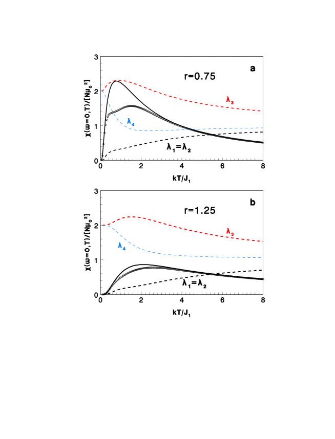
Figure 4: (color online) Temperature dependence of the static susceptibility $\chi(\omega=0,T)$ of an ANNNI chain with $J_{1}=1$, $g_{A}=g_{B}=2$, for two different values of the nnn exchange constant: (a) $J_{2}=-0.75$ and (b) $J_{2}=-1.25$, corresponding to competition ratio ${1\over 2}<r<1$ and $r>1$ respectively (strong nnn antiferromagnetism). The thick line is the exact transfer matrix result, while open circles denote the approximate calculation, Eq. (63). The temperature dependence of the eigenvalues $\lambda_{1}=\lambda_{2}$, $\lambda_{3}$ and $\lambda_{4}$ (50) is also shown by the dashed lines.

Diagonalizing the matrix of coefficients, the time dependence of the eigenmodes is found to be ($n=1,2,3,4$)

$${\cal M}_{n}(t)={\cal M}_{n}(t_{0})e^{-{{t-t_{0}}\over{\tau_{i}}}}+{\cal N}(T)f_{n}\int_{t_{0}}^{t}dt^{\prime}e^{{{t^{\prime}-t}\over{\tau_{i}}}}e^{-i\omega t^{\prime}}$$ (49)

where $\tau_{n}={1\over{\alpha\lambda_{n}}}$ are the relaxation times and $f_{1}=f_{2}=0$, $f_{3}={{g_{B}}\over 2}(g_{B}-g_{A})$, $f_{4}={{g_{B}}\over 2}(g_{B}+g_{A})$. The eigenvalues ($\lambda_{n}$) of the $4\times 4$ nonsymmetric matrix of the coefficients turn out to be independent of $g_{A}$ and $g_{B}$

$$\lambda_{1} = \lambda_{2}=1+\gamma_{2}(1-\gamma_{1}\eta_{1})+{1\over 2}\gamma_{2}\gamma_{1}(\eta_{1}+\eta_{3})$$ (50)

$$\lambda_{3} = 1+\gamma_{1}(1-\gamma_{2}\eta_{2})-\gamma_{2}(1-\gamma_{1}\eta_{1})+{1\over 2}\gamma_{2}\gamma_{1}(\eta_{1}+\eta_{3})$$ (51)

$$\lambda_{4} = 1-\gamma_{1}(1-\gamma_{2}\eta_{2})-\gamma_{2}(1-\gamma_{1}\eta_{1})+{1\over 2}\gamma_{2}\gamma_{1}(\eta_{1}+\eta_{3})$$ (52)

For non vanishing magnetic field, the time dependence of the eigenmodes is

$${\cal M}_{n}(t)={\cal N}(T){{f_{n}}\over{\lambda_{n}}}{{1}\over{1-i\omega\tau_{n}}}e^{-i\omega t}~{}~{}~{}~{}(n=1,2,3,4)$$ (53)

The relationships between the eigenmodes ${\cal M}_{n}(t)$ and the sublattice magnetizations $M_{n}(t)$ ($n=1,2,3,4$) are

$${\cal M}_{1}(t) = {1\over 2}\Big{[}M_{4}(t)-M_{2}(t)\Big{]}$$ (54)

$${\cal M}_{2}(t) = {1\over 2}\Big{[}M_{3}(t)-M_{1}(t)\Big{]}$$ (55)

$${\cal M}_{3}(t) = {1\over 4}\Big{[}\Big{(}M_{4}(t)+M_{2}(t)\Big{)}-{{g_{B}}\over{g_{A}}}\Big{(}M_{3}(t)+M_{1}(t)\Big{)}\Big{]}$$ (56)

$${\cal M}_{4}(t) = {1\over 4}\Big{[}\Big{(}M_{4}(t)+M_{2}(t)\Big{)}+{{g_{B}}\over{g_{A}}}\Big{(}M_{3}(t)+M_{1}(t)\Big{)}\Big{]}$$ (57)

and conversely

$$M_{1}(t) = {{g_{A}}\over{g_{B}}}\Big{[}{\cal M}_{4}(t)-{\cal M}_{3}(t)\Big{]}-{\cal M}_{2}(t)$$ (58)

$$M_{2}(t) = {\cal M}_{4}(t)+{\cal M}_{3}(t)-{\cal M}_{1}(t)$$ (59)

$$M_{3}(t) = {{g_{A}}\over{g_{B}}}\Big{[}{\cal M}_{4}(t)-{\cal M}_{3}(t)\Big{]}+{\cal M}_{2}(t)$$ (60)

$$M_{4}(t) = {\cal M}_{4}(t)+{\cal M}_{3}(t)+{\cal M}_{1}(t)$$ (61)

The total magnetization is

$$M_{tot}(t)=\sum_{i=1}^{4}M_{i}(t)=2{{g_{B}+g_{A}}\over{g_{B}}}{\cal M}_{4}(t)+2{{g_{B}-g_{A}}\over{g_{B}}}{\cal M}_{3}(t)=\chi(\omega)H_{0}e^{-i\omega t},$$ (62)

where the complex susceptibility $\chi(\omega,T)$ is given by

$$\chi(\omega,T) = N~{}{{\mu_{0}^{2}}\over{kT}}~{}\Big{[}1-\gamma_{1}\eta_{1}-\gamma_{2}\eta_{2}+{1\over 2}\gamma_{2}\gamma_{1}(\eta_{1}+\eta_{3})\Big{]}$$ (63)

$$\times \Bigg{[}\Big{(}{{g_{B}+g_{A}}\over 2}\Big{)}^{2}{1\over{\lambda_{4}}}{1\over{1-i\omega\tau_{4}}}+\Big{(}{{g_{B}-g_{A}}\over 2}\Big{)}^{2}{1\over{\lambda_{3}}}{1\over{1-i\omega\tau_{3}}}\Bigg{]}.$$ (64)

The approximate static susceptibility, calculated from Eq. (63) for zero frequency, is shown in Fig. 4a for ${1\over 2}<r<1$. One immediately notices that, in striking contrast with the case $0<r<{1\over 2}$ displayed in Fig. 3, the low temperature behavior of the static susceptibility is correctly reproduced.

The latter feature appears at odds with the expectation that a decoupling approximation should work better the higher the temperature. However it is worth noticing that, for the 1D ANNNI model, the $T\to 0$ asymptotic behavior of the static two-spin correlation functions is very different depending on the value of $r$. For $0<r<{1\over 2}$ both the inter- and the intra-sublattice spin-spin correlations are strong ($\eta_{1}\approx\eta_{2}\approx\eta_{3}\approx 1$, see Note notaeta, later). In contrast, for $r>{1\over 2}$ the intersublattice correlations are strong ($\eta_{2}\approx-1$, see Eq. (68) later), whereas the intrasublattice correlations are exponentially vanishing ($\eta_{1}\approx\eta_{3}\approx 0$, see Eq. (68)). At intermediate temperatures intrasublattice correlations become significant, too, and the decoupling approximation becomes less satisfactory; at high temperatures, it works well again, since all correlations (both intra- and inter-sublattice) decrease.

It should be remarked that the above considerations about the behavior of static correlation functions can not, on their own, account for the good agreement found, at low $T$, in the case ${1\over 2}<r<1$. In fact, the use of equilibrium values for the spin correlations might be questionable, since the $T=0$ Glauber dynamics does not lead to the ground state of the 1D ANNNI model in the entire region $0<r<1$.Redner To this regard, first we observe that the physical mechanism which at $T=0$ prevents the system from reaching the ground state is different, for ${1\over 2}<r<1$, with respect to the case $0<r<{1\over 2}$.Redner ; Sen ; Sen2 Next, considering that at $T=0$ a 1D model is simultaneously in the ordered phase and at its critical point, while our theory applies at $T>0$, we believe that some insight into the problem might be provided by a careful study of the role of a small but non-zero temperature on the coarsening of the 1D ANNNI model.Bray ; notaBray

In Fig. 4b the approximate static susceptibility, calculated from Eq. (63) for zero frequency in the case $r>1$, is reported. A nice overall agreement with the exact transfer matrix resultStephenson ; Harada is obtained. In this case our approximate results are expected to be quite reliable since the long-time approximation is well founded (for $r>1$, the static equilibrium state can asymptotically be reached even at $T=0$,Redner and thus the use of static spin-spin correlation functions is justified); moreover, the decoupling approximation is expected to be satisfactory both at high and low temperatures. Finally it is worth mentioning that, in the limiting case $1/r=0$ (i.e., $J_{1}=0$), the transfer matrix result for the static susceptibility is exactly reproduced by Eq. (63) for $\omega=0$ (not shown).

In Fig. 5 the temperature dependence of the amplitude of the complex susceptibility $|\chi(\omega,T)|$, obtained from Eq. (63), of an ANNNI chain with nnn antiferromagnetic coupling dominating over the nn ferromagnetic one (competition ratio $r=1.25$) is reported - for selected values of the oscillation frequency $\omega$ of the external magnetic field - both in the compensated ($g_{A}=g_{B}=2$) and uncompensated ($g_{A}\neq g_{B}$) case. No resonant behavior was observed even in the uncompensated case since, in the $T\to 0$ limit, both the zero-field static susceptibility and the relaxation times ($\tau_{3}$ and $\tau_{4}$ in Eq. (63)) fail to diverge. Thus, for low frequency, a resonance condition - similar to the one in Eq. (21) - can not be fulfilled. In the case ${1\over 2}<r<1$ a qualitatively similar behavior for $|\chi(\omega,T)|$ was found (not shown).

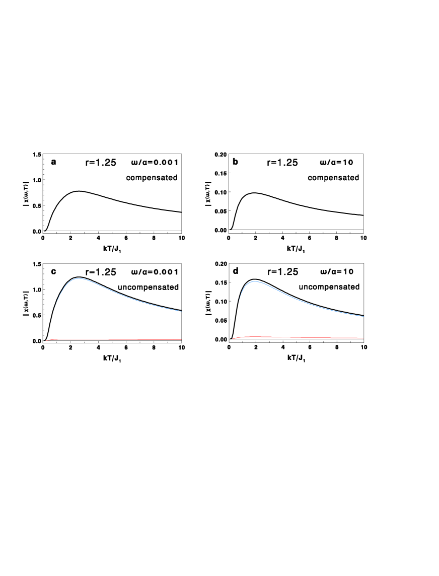
Figure 5: (color online) Temperature dependence of the amplitude of the complex susceptibility $|\chi(\omega,T)|$ for an ANNNI chain with $J_{1}=1$, $J_{2}=-1.25$ ($r=1.25$), subject to a weak external magnetic field oscillating at frequency $\omega$. Figures (a), (b) refer to the compensated case ($g_{A}=g_{B}=2$), while Figures (c) and (d) to the uncompensated case ($g_{A}=2,~{}g_{B}=3$), for selected values of the frequency ($\omega/\alpha=0.001$ and $10$). In Figs. (c,d) the thin (color) lines represent the contributions to the amplitude of the two terms on the r.h.s. of Eq. (63), while the thick (black) line is their sum. No resonant behavior is observed.

III.3 Critical dynamics of the 1D ANNNI model for $r>1$

The identification of $r=0$, $r=1$ and $1/r=0$ as dynamic critical transition points for the 1D ANNNI model with single spin-flip Glauber dynamics was recently proposed in theoretical studies of $T=0$ coarseningRedner (i.e., the relaxation of the system into the ground state after a quench from high temperature) and $T=0$ persistenceSen (i.e., the probability for a spin to remain in its original state after a quench from high temperature). In such $T=0$ studies, the dynamic critical exponent $z$ is customarily defined as the inverse of the growth exponent $n$ of the domain size

$$L(t)\simeq t^{n}\simeq t^{1/z^{\prime}}.$$ (65)

For the 1D nn Ising model, analytical calculationsBray provided $z^{\prime}=2$. For the 1D ANNNI model with $r>1$ numerical calculationsSen ; notaSen predicted a somewhat higher dynamic exponent, $z^{\prime}\simeq 2.3$. Finally, it is worth noting that Sen and Dasgupta,Sen in their study of $t=0$ persistence in the ANNNI chain, found that the dynamic critical exponent $z^{\prime}$ undergoes abrupt changes for $r=0$ (when a slight amount of nnn interaction is added to the nn one), for $1/r=0$ (when a slight amount of nn interaction is added to the nnn one), as well as for $r=1$.Sen

The fair accuracy of our approximate theoretical approach in describing the low temperature static susceptibility of the ANNNI chain with $r>1$, see Fig. 4b, encouraged us to tentatively estimate the dynamic critical exponent. However, since we work at finite temperature, rather than at $T=0$, we use a different definition, namelydaSilva ; Luscombe

$${1\over{\alpha\tau_{1}}}=\lambda_{1}\approx\Big{(}{{1}\over{\xi}}\Big{)}^{z}$$ (66)

where $\lambda_{1}$ is the smallest eigenvalue of the dynamical matrix, see Eq. (50), and $\xi$ is the static correlation length of the infinite system (the lattice constant $c$ along the chain was set to 1). For the compensated case $g_{A}=g_{B}$, the latter quantity can be analytically calculated using the transfer matrix method,Stephenson see Eq. (91), and for $r>1$ its expansion in the $T\to 0$ limit turns out to be

$$\Big{(}{{1}\over{\xi}}\Big{)}^{2}\approx{1\over 4}e^{{{2(J_{1}-2|J_{2}|)}\over{kT}}},$$ (67)

where we have explicitly taken into account that $J_{1}>0$ and $J_{2}<0$.

Taking into account the $T\to 0$ asymptotic behavior, for $r>1/2$, notaeta of the $\gamma_{i}$ and $\eta_{i}$ coefficients

$$\gamma_{1}\approx 1-2e^{-{{4J_{1}}\over{kT}}}~{}~{}~{}\gamma_{2}\approx-1+2e^{-{{4|J_{2}|}\over{kT}}}$$ (68)

$$\eta_{1}\approx{1\over 2}e^{{{J_{1}-2|J_{2}|}\over{kT}}}~{}~{}~{}\eta_{2}\approx-1+e^{{{J_{1}-2|J_{2}|}\over{kT}}}~{}~{}~{}\eta_{3}\approx-{3\over 2}e^{{{J_{1}-2|J_{2}|}\over{kT}}},$$ (69)

for the inverse of the longest relaxation time we obtain, provided that $J_{1}\neq 0$

$${1\over{\alpha\tau_{1}}}=\lambda_{1}\approx e^{{{J_{1}-2|J_{2}|}\over{kT}}}.$$ (70)

In the special case $J_{1}=0$ (i.e., $1/r=0$), letting $\gamma_{1}=0$ in Eq. (50) and using the $T\to 0$ expansion for $\gamma_{2}$ in Eq. (68), we obtain

$${1\over{\alpha\tau_{1}}}=\lambda_{1}\approx 2e^{-{{4|J_{2}|}\over{kT}}}.$$ (71)

In conclusion, within our approximate theoretical scheme, the dynamic critical exponent of the 1D ANNNI chain with competing nn and nnn exchange interactions was found to be $z=1$ for any finite $r>1$, while in the absence of competing interactions (i.e., for $r=0$ and $1/r=0$) we found $z=2$. Notice that, for the 1D Ising model with exchange limited to the nn ($r=0$), the value $z=2$, obtained using the definition in Eq. (66),Luscombe coincides with the value $z^{\prime}=2$, obtained using the definition in Eq. (65).Bray This appears not to be the case for the 1D ANNNI model with $1<r<+\infty$, where the values $z=1$ (present work) and $z^{\prime}\simeq 2.3$ (References Sen, ; notaSen, ) were found. In order to ascertain the origin of this discrepancy, we believe that it would be useful to study the role of a small but non-zero temperature ($T>0$) on the coarsening dynamics of the 1D ANNNI model.notaBray

IV Conclusions

In conclusion, in this paper we have studied the effect of antiferromagnetic interactions on the single spin-flip Glauber dynamics of two different one-dimensional (1D) Ising models with spin $\pm 1$. For the first model, an Ising chain with antiferromagnetic exchange interaction limited to nearest neighbors and subject to an oscillating magnetic field, the system of master equations describing the time evolution of sublattice magnetizations can easily be solved within a linear field approximation and a long time limit. Resonant behavior of the magnetization as a function of temperature (stochastic resonance) is found, at low frequency, only when spins on opposite sublattices are uncompensated owing to different gyromagnetic factors (i.e., in the presence of a ferrimagnetic short range order). For the second model, the axial next-nearest neighbor Ising (ANNNI) chain, where the nnn antiferromagnetic exchange coupling is assumed to compete with the nn ferromagnetic one, the long time response of the model to a weak, oscillating magnetic field is investigated in the framework of a decoupling approximation for three-spin correlation functions, which is required to close the system of master equations. Within such approximate theoretical scheme, the $T=0$ dynamics of the Ising-Glauber chain with competing interactions is found to be in a different universality class than that of the Ising chain with antiferromagnetic exchange limited to nearest neighbors ($r=0$) or limited to next-nearest neighbors ($1/r=0$). In particular, we find an abrupt change in the $T=0$ dynamic behavior of the model in the neighborhood of the dynamic critical point $1/r=0$ since, when a slight amount of ferromagnetic nn exchange is added to the antiferromagnetic nnn exchange, we find that the critical exponent $z$, defined by Eq. (66), changes abruptly from $z=2$ to $z=1$. Considering that $z=2$ is also the value of the dynamic critical exponent for the unfrustrated nn Ising chain, one might expect similar abrupt changes in $z$ to occur also in the neighborhood of the dynamic critical points $r=0$ (i.e. when a slight amount of AF nnn exchange is added to the nn F exchange) and $r=1$, as suggested by studies of $T=0$ coarsening dynamicsRedner and $T=0$ persistenceSen in the ANNNI chain. Unfortunately, the inaccuracy of our approximate theoretical scheme in reproducing the static susceptibility of the 1D ANNNI model with $0<r\leq 1$ for low temperature prevented us from calculating the dynamic critical exponent in this range of the competition ratio.

Appendix A Analytic transfer matrix results for the static properties of 1D Ising models

A.1 The 1D nearest neighbor Ising model with alternating spins in a static field

In this subsection we calculate, within the transfer matrix formalism,Stanley the static properties of the 1D Ising model, Eq. (1), with nearest neighbor coupling $J$ of either sign, subject to a static magnetic field $H$ (i.e., $\omega=0$). Two types of spins with different gyromagnetic factors ($g_{A}\neq g_{B}$) are assumed to alternate along the chain. Taking periodic boundary conditions, the partition function of the chain of length $N$ (with $N$ even without loss of generality) can be expressed as

$$Z_{N}={\rm Tr}\big{(}e^{-{{\cal H}\over{kT}}}\big{)}=\sum_{\sigma_{1}=\pm 1}\sum_{\sigma_{2}=\pm 1}\cdots\sum_{\sigma_{N}=\pm 1}K(\sigma_{1},\sigma_{2})L(\sigma_{2},\sigma_{3})\cdots K(\sigma_{N-1},\sigma_{N})L(\sigma_{N},\sigma_{1})$$ (72)

where, letting ${\cal J}=J/(kT)$, $h_{A}=(g_{A}\mu_{0}H_{0})/(kT)$, $h_{B}=(g_{B}\mu_{0}H_{0})/(kT)$, the two different kernels $K$ and $L$ are defined as

$$K(\sigma_{2i-1},\sigma_{2i})=e^{{\cal J}\sigma_{2i-1}\sigma_{2i}}e^{{1\over 2}(h_{A}\sigma_{2i-1}+h_{B}\sigma_{2i})}~{}~{}~{}~{}L(\sigma_{2i},\sigma_{2i+1})=e^{{\cal J}\sigma_{2i}\sigma_{2i+1}}e^{{1\over 2}(h_{B}\sigma_{2i}+h_{A}\sigma_{2i+1})}.$$ (73)

Summing over the even sites, $Z_{N}$ can be expressed as

$$Z_{N}=\big{(}\Lambda_{+}\big{)}^{N\over 2}+\big{(}\Lambda_{-}\big{)}^{N\over 2}$$ (74)

in terms of the eigenvalues

$$\Lambda_{\pm} = e^{2{\cal J}}\cosh(h_{A}+h_{B})+e^{-2{\cal J}}\cosh(h_{A}-h_{B})\pm$$ (75)

$$\pm \sqrt{e^{4{\cal J}}\cosh^{2}(h_{A}+h_{B})+e^{-4{\cal J}}\cosh^{2}(h_{A}-h_{B})+2\cosh(h_{A}+h_{B})\cosh(h_{A}-h_{B})+2-e^{4{\cal J}}-e^{-4{\cal J}}}$$ (77)

of the real symmetric $2\times 2$ matrix

$$S=\left(\begin{array}[]{cc}e^{2{\cal J}+h_{A}+h_{B}}+e^{-2{\cal J}+h_{A}-h_{B}}&e^{h_{B}}+e^{-h_{B}}\\ e^{h_{B}}+e^{-h_{B}}&e^{2{\cal J}-h_{A}-h_{B}}+e^{-2{\cal J}-h_{A}+h_{B}}\end{array}\right).$$ (78)

It is immediate to verify that, in the limit $g_{A}=g_{B}$, the well-known result for the 1D nn Ising chain in a static external field is recovered.Stanley In the thermodynamic limit $N\to\infty$, only the larger eigenvalue $\Lambda_{+}$ matters, $Z_{N}\to(\Lambda_{+})^{N\over 2}$, and the static susceptibility in zero field can be expressed in terms of its second derivative with respect to the field $H$

$$\chi(\omega=0,T)={N\over 2}kT\Big{[}{1\over{\Lambda_{+}}}{{\partial^{2}\Lambda_{+}}\over{\partial H^{2}}}\Big{]}_{H=0}={{N\mu_{0}^{2}}\over{kT}}\Big{[}\Big{(}{{g_{A}+g_{B}}\over 2}\Big{)}^{2}e^{{2J}\over{kT}}+\Big{(}{{g_{A}-g_{B}}\over 2}\Big{)}^{2}e^{-{2J}\over{kT}}\Big{]}.$$ (79)

A.2 The 1D ANNNI model in zero field

In this subsection we collect, for the reader’s convenience, some exact results for the static properties of the 1D ANNNI model in zero field, Eq. (23), which were obtained by StephensonStephenson and HaradaHarada in the case of a linear chain with $N$ identical spins ($g_{A}=g_{B}=g$ and $\sigma=\pm 1$). Using the transfer matrix method, the partition function can be exactly expressed as

$$Z_{N}=(\lambda_{+})^{N}+(\lambda_{-})^{N}$$ (80)

in terms of the eigenvalues of the symmetric $2\times 2$ matrix

$$S=\left(\begin{array}[]{cc}a&c\\ c&b\end{array}\right)=\left(\begin{array}[]{cc}e^{{{J_{2}+J_{1}}\over{kT}}}&e^{{{J_{2}-J_{1}}\over{kT}}}\\ e^{{{J_{2}-J_{1}}\over{kT}}}&e^{-{{J_{2}}\over{kT}}}\end{array}\right)$$ (81)

The eigenvalues take the formStephenson

$$\lambda_{\pm}={1\over 2}[a+b\pm\Delta]=e^{{{J_{2}}\over{kT}}}\Big{[}\cosh\Big{(}{{J_{1}}\over{kT}}\Big{)}\pm\sqrt{\sinh^{2}\Big{(}{{J_{1}}\over{kT}}\Big{)}+e^{-{{4J_{2}}\over{kT}}}}\Big{]}$$ (82)

where

$$\Delta=\sqrt{(a-b)^{2}+4c^{2}}=2e^{{{J_{2}}\over{kT}}}\sqrt{\sinh^{2}\Big{(}{{J_{1}}\over{kT}}\Big{)}+e^{-{{4J_{2}}\over{kT}}}}.$$ (83)

Both $\lambda_{+}$ and $\Delta$ are always real positive quantities.

In the thermodynamic limit $N\to\infty$, the static two spin correlation function $\eta_{n}$ take the formStephenson

$$\eta_{n}=\langle\sigma_{j}\sigma_{j+n}\rangle={1\over{2\big{(}\lambda_{+}\big{)}^{n}}}\Big{[}\big{(}\mu_{+}\big{)}^{n}\Big{(}\ 1+{{a^{2}-b^{2}}\over{\Delta\Delta^{\prime}}}\Big{)}+\big{(}\mu_{-}\big{)}^{n}\Big{(}\ 1-{{a^{2}-b^{2}}\over{\Delta\Delta^{\prime}}}\Big{)}\Big{]}$$ (84)

where the quantities $\Delta^{\prime}$, defined as

$$\Delta^{\prime}=\sqrt{(a+b)^{2}-4c^{2}}=2e^{{{J_{2}}\over{kT}}}\sqrt{\cosh^{2}\Big{(}{{J_{1}}\over{kT}}\Big{)}-e^{-{{4J_{2}}\over{kT}}}},$$ (85)

and

$$\mu_{\pm}=e^{{{J_{2}}\over{kT}}}\Big{[}\sinh\Big{(}{{J_{1}}\over{kT}}\Big{)}\pm\sqrt{\cosh^{2}\Big{(}{{J_{1}}\over{kT}}\Big{)}-e^{-{{4J_{2}}\over{kT}}}}\Big{]}$$ (86)

may be complex. More precisely, the quantities $\mu_{\pm}$ are real for $T<T_{D}$ and complex conjugates for $T>T_{D}$. $T_{D}$ is the so-called disorder point, defined by the equation $\Delta^{\prime}(T_{D})=0$, which has solutions for $0<r<1/2$ at some finite temperature $T_{D}$. For $T<T_{D}$ the static equilibrium two-spin correlation functions $\eta_{n}=\langle\sigma_{j}\sigma_{j+n}\rangle$ present a monotonic exponential decay, while for $T>T_{D}$ they have an oscillating exponential decay.Stephenson

Summing over all pair correlations, the exact zero field static susceptibility can be expressed asStephenson

$$\chi(\omega=0,T)=\Big{(}{{{g^{2}\mu_{0}}^{2}}\over{kT}}\Big{)}\Big{(}{{a+b}\over{\Delta}}\Big{)}\Big{[}{{a(a-b+\Delta)+2c^{2}}\over{b(b-a+\Delta)+2c^{2}}}\Big{]}.$$ (87)

The wave-vector dependent susceptibility, defined as

$$\chi(q)=N{{g^{2}\mu_{0}^{2}}\over{kT}}\sum_{n}\langle\sigma_{j}\sigma_{j+n}\rangle e^{iqn}$$ (88)

presents a maximum at a wave-vector $q_{m}$, which is given byHarada

$$\cos q_{m}={{(\mu_{+}+\mu_{-})(\lambda_{+}-\lambda_{-})}\over{4\mu_{+}\mu_{-}}}$$ (89)

For $0<r<1/4$ one has $q_{m}=0$ at all temperatures , while for $1/4<r<1/2$ there is a definite temperature $T_{L}$ ($\neq T_{D}$) above which $q_{m}\neq 0$, whereas for $T<T_{L}$ $q_{m}=0$. When $1/2<r$, one has $q_{m}(T=0)=\pi/2$. In the limit of $T\to\infty$, $q_{m}$ tends to the mean field value $\cos q_{m}=1/(4r)$. Expanding $\chi(q)$ in the neighborhood of $q_{m}$ up to second order in $\Delta q=q_{m}-q$, one obtains a Lorentzian form, and the correlation length $\xi$ can be defined in terms of its full width at half maximum as

$$\chi(q)={{\chi(q_{m})}\over{1+\xi^{2}(\Delta q)^{2}}}$$ (90)

and turns out to be

$$\Big{(}{1\over{\xi}}\Big{)}^{2} = {{(\lambda_{+}-\lambda_{-}-\mu_{+}-\mu_{-})^{2}}\over{(\mu_{+}+\mu_{-})(\lambda_{+}-\lambda_{-})-4\mu_{+}\mu_{-}}}~{}~{}~{}{\rm for}~{}q_{m}=0,$$ (91)

$$\Big{(}{1\over{\xi}}\Big{)}^{2} = {{(\mu_{+}-\mu_{-})^{2}(\lambda_{+}+\lambda_{-})^{2}}\over{(\mu_{+}+\mu_{-})^{2}(\lambda_{+}-\lambda_{-})^{2}-16\mu_{+}^{2}\mu_{-}^{2}}}~{}~{}~{}{\rm for}~{}q_{m}\neq 0.$$ (92)

For $1/4<r<1/2$, it turns out that at $T_{L}$ the correlation length becomes zero, which is a characteristic of the Lifshitz point.RednerStanley

References

- (1) R. Benzi, G. Parisi, A. Sutera and A. Vulpiani, Tellus 34, 10 (1982); SIAM J. Appl. Math. 43, 565 (1983).
- (2) L. Gammaitoni, F. Marchesoni, E. Menichella-Saetta and S. Santucci, Phys. Rev. Lett. 62, 349 (1989).
- (3) L. Gammaitoni, P. Hänggi, P. Jung and F. Marchesoni, Rev. Mod. Phys. 70, 223 (1998).
- (4) U. Siewert and L. Schimansky-Geier, Phys. Rev. E 58, 2843 (1998).
- (5) R. J. Glauber, J. Math. Phys. 4, 294 (1963).
- (6) J. J. Brey and A. Prados, Phys. Lett. A 216, 240 (1996).
- (7) Z. Néda, Phys. Rev. E 51, 5315 (1995).
- (8) Z. Néda, Phys. Lett. A 210, 125 (1996).
- (9) Kwan-tai Leung and Z. Néda, Phys. Lett. A 246, 505 (1998).
- (10) Z. R. Yang, Phys. Rev. B 46, 11578 (1992).
- (11) J. Kamphorst Leal da Silva, Adriana G. Moreira, M. Silvério Soares, and F. C. Sá Barreto, Phys. Rev. E 52, 4527 (1995).
- (12) A. Caneschi, D. Gatteschi, N. Lalioti, C. Sangregorio, R. Sessoli, G. Venturi, A. Vindigni, A. Rettori, M. G. Pini and M. A. Novak, Angew. Chem., Int. Ed. Engl. 40, 1760 (2001).
- (13) A. Caneschi, D. Gatteschi, N. Lalioti, C. Sangregorio, R. Sessoli, G. Venturi, A. Vindigni, A. Rettori, M. G. Pini and M. A. Novak, Europhys. Lett. 58, 771 (2002).
- (14) L. Bogani, C. Sangregorio, R. Sessoli and D. Gatteschi, Angew. Chem. Int. Ed. 44, 5817 (2005).
- (15) K. Bernot, L. Bogani, A. Caneschi, D. Gatteschi and R. Sessoli, J. Am. Chem. Soc. 128, 7947 (2006).
- (16) A. Vindigni, N. Regnault and Th. Jolicoeur, Phys. Rev. B 70, 134423 (2004).
- (17) W. Selke, Physics Reports 170, 213 264 (1988).
- (18) T. Morita and T. Horiguchi, Phys. Lett. A 38, 223 (1972).
- (19) In contrast with the equilibrium case, the dynamics of the 1D ANNNI model in zero field is not equivalent to that of a 1D nearest neighbor Ising model in an effective external field: see Ref. Yang, .
- (20) J.-J. Kim, S. Mori and I. Harada, Phys. Lett. A 202, 68 (1995).
- (21) J. Stephenson, Can. J. Phys. 48, 1724 (1970).
- (22) I. Harada, J. Phys. Soc. Jpn
- (23) M. G. Pini and A. Rettori, Phys. Rev. B 48, 3240 (1993).
- (24) J.-J. Kim, S. Mori and I. Harada J. Phys. Soc. Japan 65, 2624 (1996).
- (25) S. Redner and P. L. Krapivsky, J. Phys. A 31, 9929 (1998).
- (26) A. J. Bray, J. Phys. A: Math. Gen. 22, L67 (1989).
- (27) P. Sen and S. Dasgupta, J. Phys. A 37, 11949 (2004).
- (28) P. Sen and P. K. Das, in Quantum Annealing and Related Optimization Methods, edited by A. Das and B. K. Chakrabarti, Lecture Notes in Physics 679 (Springer, New York, 2005), (arXiv:cond-mat/0505027).
- (29) While for the 1D nn Ising model such a study was performed by Bray,Bray for the 1D ANNNI model it has not yet been performed, to our knowledge, and is deferred to future work.
- (30) It is worth noting that such a value, , for the growth exponent turns out to be in close agreement with previous analytical predictions, obtained by Redner and KrapivskyRedner in the same regime of strong nnn antiferromagnetic exchange. In fact for the latter authors estimated the density of domains of length 3 and 1 to scale as and , respectively. For , it turns out that the average of and (which is inversely proportional to the domain size ) scales just as .
- (31) James H. Luscombe, Marshall Luban and Joseph P. Reynolds, Phys. Rev. E 53, 5852 (1996).
- (32) In the case of ferromagnetic ground state, , the asymptotic behavior of the correlation functions for the 1D ANNNI model in zero field is instead: , , .
- (33) H. E. Stanley, in Introduction to Phase Transitions and Critical Phenomena, (Clarendon Press, Oxford, 1971), p. 115 and p. 131.
- (34) S. Redner and H. E. Stanley, Phys. Rev. B 16, 4901 (1977).