On the definition of the $\Delta$ mass and width

Abstract

In the framework of effective field theory we show that, at two-loop order, the mass and width of the $\Delta$ resonance defined via the (relativistic) Breit-Wigner parametrization both depend on the choice of field variables. In contrast, the complex-valued position of the pole of the propagator is independent of this choice.

The problem of defining masses of unstable particles has a long history. A popular definition corresponding to a (relativistic) Breit-Wigner formula makes use of the zero of the real part of the inverse propagator to identify the mass. The field-redefinition dependence of such a definition was shown in Refs. Willenbrock:1990et ; Valencia:1990jp in the scalar sector of the Standard Model. Another important example is the definition of the $Z$-boson mass. The gauge-parameter dependence of the Breit-Wigner mass starting at two-loop order was shown in Refs. Sirlin:1991fd ; Sirlin:1991rt ; Willenbrock:1991hu ; Gegelia:1992kj ; Gambino:1999ai . In contrast, defining the mass and width in terms of the complex-valued position of the pole of the propagator leads to both field-redefinition and gauge-parameter independence 'tHooft:1972ue ; Lee:1972fj ; Balian:1976vq .

It was noted in Ref. Willenbrock:1991hu that, as there is no fundamental theory of baryon resonances, the issue of field-redefinition invariance and gauge-parameter (in)dependence does not arise for unstable particles of this kind. As these resonances are thought to be described by QCD, with the progress of lattice techniques and, especially, the low-energy effective theories (EFT) of QCD (see, e.g., Weinberg:1979kz ; Gasser:1983yg ; Gasser:1988rb ; Scherer:2005ri ; Hemmert:1997ye ; Hacker:2005fh ; Pascalutsa:2006up and references therein) the question of defining resonance masses becomes important. In this letter we examine this issue for the $\Delta$ resonance. As discussed in Ref. Hoehler , the conventional resonance mass and width determined from generalized Breit-Wigner formulas have problems regarding their relation to S-matrix theory and suffer from a strong model dependence. Here, we will show that these parameters, in addition, depend on the field-redefinition parameter in a low-energy EFT of QCD.

For simplicity we ignore isospin and consider an EFT of a single nucleon, pion, and $\Delta$ resonance. Defining

$$\Lambda_{\mu\nu}=-(i\not{\partial}-m_{\Delta})g_{\mu\nu}+i\,(\gamma_{\mu}\partial_{\nu}+\gamma_{\nu}\partial_{\mu})-i\gamma_{\mu}\not{\partial}\gamma_{\nu}-m_{\Delta}\gamma_{\mu}\gamma_{\nu},$$

the free Lagrangian is given by

$$\mathcal{L}_{0}=\bar{\psi}^{\mu}\,\Lambda_{\mu\nu}\,\psi^{\nu}+\bar{\Psi}(i\not{\partial}-m_{N})\Psi+\frac{1}{2}\,\partial_{\mu}\pi\partial^{\mu}\pi\,.$$ (1)

Here, the vector-spinor $\psi^{\mu}$ describes the $\Delta$ in the Rarita-Schwinger formalism Rarita:1941mf , $\Psi$ stands for the nucleon field with mass $m_{N}$, and $\pi$ represents the pion field which we take massless to simplify the calculations. The most general (free) Rarita-Schwinger Lagrangian contains an arbitrary parameter $A$. In a consistent theory having the right number of degrees of freedom, physical observables do not depend on $A$ Wies:2006rv and we have chosen a convenient value, namely $A=-1$. We consider the interaction terms of the form

$$\mathcal{L}_{\rm int}=g\,\partial^{\nu}\pi\,\bar{\psi}^{\mu}\left(g_{\mu\nu}-z\gamma_{\mu}\gamma_{\nu}\right)\Psi+\mbox{H.c.}+\cdots\,,$$ (2)

where the ellipsis refers to an infinite number of interaction terms which are present in the EFT. These terms also include all counter-terms which take care of divergences appearing in our calculations. The consistency of the interaction terms with the constraints of the spin-3/2 system fixes the value of the parameter $z$ to $-1$ for $A=-1$ Nath:1971wp ; Hacker:2005fh . Throughout this paper we use dimensional regularization. Although our results are renormalization scheme independent, for simplicity we use the minimal subtraction scheme cbare . It is implemented by subtracting the divergent parts of one- and two-loop diagrams using the standard procedure Collins:1984xc .

Let us consider the field transformation

$$\bar{\psi}^{\mu}\to\bar{\psi}^{\mu}+\xi\,\partial^{\mu}\pi\bar{\Psi}\,,\quad\psi^{\nu}\to\psi^{\nu}+\xi\,\partial^{\nu}\pi\Psi\,,$$ (3)

where $\xi$ is an arbitrary real parameter. When inserted into the Lagrangians of Eqs. (1) and (2), the field redefinition generates additional interaction terms. The terms linear in $\xi$ are given by

$$\mathcal{L}_{\rm add\,int}=\xi\,\partial^{\mu}\pi\,\bar{\Psi}\,\Lambda_{\mu\nu}\,\psi^{\nu}+\xi\,\partial^{\nu}\pi\,\bar{\psi}^{\mu}\,\Lambda_{\mu\nu}\,\Psi\,.$$ (4)

Note that the contribution generated from the expression explicitly shown in Eq. (2) vanishes identically. Because of the equivalence theorem physical quantities cannot depend on the field redefinition parameter $\xi$. Below we demonstrate that the complex-valued position of the pole of the $\Delta$ propagator does not depend on $\xi$. In contrast, the mass and width defined via (the zero of) the real and imaginary parts of the inverse propagator depend on $\xi$ at two-loop order.

The dressed propagator of the $\Delta$ in $n$ space-time dimensions can be written as Hacker:2005fh ; note

$$- i\left[g^{\mu\nu}-\frac{\gamma^{\mu}\gamma^{\nu}}{n-1}-\frac{p^{\mu}\gamma^{\nu}-\gamma^{\mu}p^{\nu}}{(n-1)m_{\Delta}}-\frac{(n-2)p^{\mu}p^{\nu}}{(n-1)m_{\Delta}^{2}}\right]$$ (5)

$$\times\frac{1}{p/\hskip 1.00006pt-m_{\Delta}-\Sigma_{1}-p/\hskip 1.00006pt\Sigma_{6}}+\mbox{pole-free terms}\,,$$

where we parameterized the self-energy of the $\Delta$ as

$$\Sigma_{1}(p^{2})g^{\mu\nu}+\Sigma_{2}(p^{2})\gamma^{\mu}\gamma^{\nu}+\Sigma_{3}(p^{2})p^{\mu}\gamma^{\nu}+\Sigma_{4}(p^{2})\gamma^{\mu}p^{\nu}$$

$$+\Sigma_{5}(p^{2})\,p^{\mu}p^{\nu}+\Sigma_{6}(p^{2})\,p/\hskip 1.00006ptg^{\mu\nu}+\Sigma_{7}(p^{2})\,p/\hskip 1.00006pt\gamma^{\mu}\gamma^{\nu}$$

$$+\Sigma_{8}(p^{2})\,p/\hskip 1.00006ptp^{\mu}\gamma^{\nu}+\Sigma_{9}(p^{2})\,p/\hskip 1.00006pt\gamma^{\mu}p^{\nu}+\Sigma_{10}(p^{2})\,p/\hskip 1.00006ptp^{\mu}p^{\nu}.$$ (6)

The complex pole $z$ of the $\Delta$ propagator is obtained by solving the equation

$$z-m_{\Delta}-\Sigma_{1}(z^{2})-z\,\Sigma_{6}(z^{2})=0\,.$$ (7)

The pole mass is defined as the real part of $z$.

On the other hand, the mass $m_{R}$ and width $\Gamma$ of the $\Delta$ resonance are often determined from the real and imaginary parts of the inverse propagator (corresponding to the Breit-Wigner parametrization), i.e.,

$$m_{R}-m_{\Delta}-{\rm Re}\,\Sigma_{1}(m_{R}^{2})-m_{R}\,{\rm Re}\,\Sigma_{6}(m_{R}^{2})=0\,,$$

$$\Gamma=-2\,{\rm Im}\,\Sigma_{1}(m_{R}^{2})-2\,m_{R}\,{\rm Im}\,\Sigma_{6}(m_{R}^{2})\,.$$ (8)

Below we calculate the $\Delta$ mass using both definitions and analyze their $\xi$ dependence to first order.

The $\Delta$ self-energy at one loop-order is given by the diagram in Fig. 1 (a). The corresponding results for $\Sigma_{1}$ and $\Sigma_{6}$ read

$$\Sigma_{1}^{(a)} = -g^{2}\,m_{N}\,I_{1}-2\xi\,g\left[\left(p^{2}-m_{\Delta}m_{N}\right)I_{1}+p^{2}J_{1}\right],$$

$$\Sigma_{6}^{(a)} = -g^{2}\left(I_{1}+J_{1}\right)+2\xi\,g\left[m_{\Delta}J_{1}+\left(m_{\Delta}-m_{N}\right)I_{1}\right]\,,$$

where $I_{1}$, $J_{1}$ are defined through the one-loop integrals note2

$$I^{\alpha\beta}\,,I^{\alpha\beta\gamma} = \int\frac{i\,d^{n}k}{(2\,\pi)^{n}}\frac{k^{\alpha}k^{\beta},k^{\alpha}k^{\beta}k^{\gamma}}{\left[k^{2}+i\,0^{+}\right]\left[\left(p+k\right)^{2}-m_{N}^{2}+i\,0^{+}\right]},$$

which we parameterize as

$$I^{\alpha\beta} = I_{1}g^{\alpha\beta}+I_{2}p^{\alpha}p^{\beta}\,,$$

$$I^{\alpha\beta\gamma} = J_{1}\left(g^{\alpha\beta}p^{\gamma}+g^{\alpha\gamma}p^{\beta}+g^{\beta\gamma}p^{\alpha}\right)+J_{2}p^{\alpha}p^{\beta}p^{\gamma}.$$

The two-loop contributions to the $\Delta$ self-energy are given in Fig. 1 (b) - (d). We are interested in terms linear in $\xi$. Calculating diagram (b) and (c) we find that they give vanishing contributions. The result of diagram (d), linear in $\xi$, can be reduced to the form

$$\Sigma_{1}^{(d)} = 2\,g^{3}\xi\,\left[m_{N}^{2}I_{1}^{2}+p^{2}\left(I_{1}+J_{1}\right)^{2}\right]\,,$$

$$\Sigma_{6}^{(d)} = 4\,g^{3}\,\xi\,m_{N}\,I_{1}\left(I_{1}+J_{1}\right)\,.$$ (10)

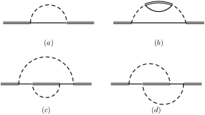
Figure 1: $\Delta$ self-energy diagrams. Solid, dashed, and double lines correspond to nucleon, pion, and $\Delta$, respectively.

Note that the vanishing of the contributions of diagrams (b) and (c) as well as the simple expression of Eq. (10) have to be attributed to the special choice of the field transformation of Eq. (3).

To find the pole of the propagator we insert its loop expansion

$$z=m_{\Delta}+\delta_{1}z+\delta_{2}z+\cdots\,$$ (11)

in Eq. (7) and solve the resulting equation order by order. Using Eq. (LABEL:DsePar) we obtain for the one-loop result

$$\delta z_{1} = -g^{2}\,\left[m_{\Delta}\bar{J}_{1}+\left(m_{\Delta}+m_{N}\right)\bar{I}_{1}\right]\,,$$ (12)

$$\bar{J}_{1}=J_{1}|_{p^{2}=m_{\Delta}^{2}}\,,\ \ \ \bar{I}_{1}=I_{1}|_{p^{2}=m_{\Delta}^{2}}.$$

The contribution to the two-loop expression $\delta z_{2}$, linear in $\xi$, generated by the one-loop diagram reads

$$\delta z_{2,1L}^{\xi}=2\,g^{3}\,\xi\,\left[m_{\Delta}\bar{J}_{1}+\left(m_{\Delta}+m_{N}\right)\bar{I}_{1}\right]^{2}\,.$$ (13)

For the genuine two-loop contribution to $\delta z_{2}$ we have

$$\delta z_{2,2L}^{\xi}=-2\,g^{3}\,\xi\,\left[m_{\Delta}\bar{J}_{1}+\left(m_{\Delta}+m_{N}\right)\bar{I}_{1}\right]^{2}.$$ (14)

These two contributions exactly cancel each other leading to the $\xi$-independent pole of the propagator.

We perform the same analysis inserting the loop expansion of $m_{R}$,

$$m_{R}=m_{\Delta}+\delta_{1}m+\delta_{2}m+\cdots,$$ (15)

in Eq. (8). For $\delta m_{1}$ we obtain

$$\delta m_{1}=-g^{2}\,\left[m_{\Delta}{\rm Re}\,\bar{J}_{1}+\left(m_{\Delta}+m_{N}\right){\rm Re}\,\bar{I}_{1}\right]\,.$$ (16)

The contribution to $\delta m_{2}$ generated by the one-loop diagram reads

$$\delta m_{2,1L}^{\xi}=2\,g^{3}\,\xi\,\left[m_{\Delta}{\rm Re}\,\bar{J}_{1}+\left(m_{\Delta}+m_{N}\right){\rm Re}\,\bar{I}_{1}\right]^{2}\,.$$ (17)

For the two-loop contribution to $\delta m_{2}$ we have

$$\delta m_{2,2L}^{\xi}=-2\,g^{3}\,\xi\,{\rm Re}\left[m_{\Delta}\bar{J}_{1}+\left(m_{\Delta}+m_{N}\right)\bar{I}_{1}\right]^{2}.$$ (18)

For an unstable $\Delta$ resonance $\bar{I}_{1}$ and $\bar{J}_{1}$ have imaginary parts and therefore Eqs. (17) and (18) do not cancel each other, thus leading to a $\xi$-dependent mass $m_{R}$. An analogous result holds for the width $\Gamma$ obtained from Eq. (8).

To conclude, we addressed the issue of defining the mass and width of the $\Delta$ resonance in the framework of a low-energy EFT of QCD. In general, the scattering amplitude of a resonant channel can be presented as a sum of the resonant contribution expressed in terms of the dressed propagator of the resonance and the background contribution. The resonant contribution defines the Breit-Wigner parameters through the real and imaginary parts of the inverse (dressed) propagator. The resonant part and the background separately depend on the chosen field variables, while the sum is of course independent of this choice. We have performed a particular field transformation with an arbitrary parameter $\xi$ in the effective Lagrangian. In a two-loop calculation we have demonstrated that the mass and width of the $\Delta$ resonance determined from the real and imaginary parts of the inverse propagator depend on the choice of field variables. On the other hand, the complex pole of the full propagator does not depend on the field transformation parameter $\xi$.

Note that according to general theorems Chisholm:1961 ; Kamefuchi:1961sb ; Coleman:1969sm ; Weinberg:1995mt it is expected that in quantum field theories the $S$-matrix is independent of field redefinitions (change of variables). The pole of the $\Delta$ propagator corresponds to the pole of the $S$-matrix. The Laurent-series expansion of the $S$-matrix around this pole has to be independent of the field redefinition term-by-term. Therefore the pole of the $\Delta$ propagator is expected to be independent of the field redefinition.

The conclusions from this work are not restricted to the considered toy model or EFT in general. Rather, our results are a manifestation of the general feature that the (relativistic) Breit-Wigner parametrization leads to model- and process-dependent masses and widths of resonances. Although in some cases (like the $\Delta$ resonance) the background has small numerical effect on the Breit-Wigner mass, still the pole mass and the width should be considered preferable as these are free of conceptual ambiguities. This agrees with and supports the recent results of Ref. Bohm:2004zi .

- (1) S. Willenbrock and G. Valencia, Phys. Lett. B 247, 341 (1990).
- (2) G. Valencia and S. Willenbrock, Phys. Rev. D 42, 853 (1990).
- (3) A. Sirlin, Phys. Rev. Lett. 67, 2127 (1991).
- (4) A. Sirlin, Phys. Lett. B 267, 240 (1991).
- (5) S. Willenbrock and G. Valencia, Phys. Lett. B 259, 373 (1991).
- (6) J. Gegelia, G. Japaridze, A. Tkabladze, A. Khelashvili and K. Turashvili, in Quarks ’92, Proceedings of the International Seminar on Quarks, Zvenigorod, Russia, 1992, edited by D. Yu. Grigoriev, V. A. Matveev, V. A. Rubakov, and P. G. Tinyakov (World Scientific, River Edge, N. J., 1993), ArXiv:hep-ph/9910527.
- (7) P. Gambino and P. A. Grassi, Phys. Rev. D 62, 076002 (2000).
- (8) G. ’t Hooft and M. J. G. Veltman, Nucl. Phys. B50, 318 (1972).
- (9) B. W. Lee and J. Zinn-Justin, Phys. Rev. D 5, 3121 (1972).
- (10) D. Gross, in Methods in Field Theory, edited by R. Balian and J. Zinn-Justin (North-Holland, Amsterdam, 1976).
- (11) S. Weinberg, Physica A96, 327 (1979).
- (12) J. Gasser and H. Leutwyler, Annals Phys. 158, 142 (1984).
- (13) J. Gasser, M. E. Sainio, and A. Švarc, Nucl. Phys. B307, 779 (1988).
- (14) S. Scherer, Adv. Nucl. Phys. 27, 277 (2003); S. Scherer and M. R. Schindler, arXiv:hep-ph/0505265.
- (15) T. R. Hemmert, B. R. Holstein, and J. Kambor, J. Phys. G 24, 1831 (1998).
- (16) C. Hacker, N. Wies, J. Gegelia, and S. Scherer, Phys. Rev. C 72, 055203 (2005).
- (17) V. Pascalutsa, M. Vanderhaeghen, and S. N. Yang, Phys. Rept. 437, 125 (2007).
- (18) G. Höhler, Against Breit-Wigner parameters — a pole-emic, in C. Caso et al. [Particle Data Group], Eur. Phys. J. C 3, 624 (1998).
- (19) W. Rarita and J. S. Schwinger, Phys. Rev. 60, 61 (1941).
- (20) N. Wies, J. Gegelia, and S. Scherer, Phys. Rev. D 73, 094012 (2006).
- (21) L. M. Nath, B. Etemadi and J. D. Kimel, Phys. Rev. D 3, 2153 (1971).
- (22) For the purposes of this work we could have also worked in terms of bare parameters. In this case no counter term diagrams occur and the loop integrals do not need to be subtracted.
- (23) J. C. Collins, Renormalization (Cambridge University Press, Cambridge, UK, 1984).
- (24) The fomulas of Ref. Hacker:2005fh are given in 4 dimensions but can be easily generalized for dimensions.
- (25) The loop integrals and are made finite by applying the minimal subtraction scheme, i.e., by subtracting the parts proportional to .
- (26) J. Chisholm, Nucl. Phys. 26, 469 (1961).
- (27) S. Kamefuchi, L. O’Raifeartaigh and A. Salam, Nucl. Phys. 28, 529 (1961).
- (28) S. R. Coleman, J. Wess and B. Zumino, Phys. Rev. 177, 2239 (1969).
- (29) S. Weinberg, The Quantum theory of fields. Vol. 1: Foundations (Cambridge University Press, Cambridge, UK, 1995).
- (30) A. R. Bohm and Y. Sato, Phys. Rev. D 71, 085018 (2005).