Chromospheric Dynamics and Line Formation

Abstract

The solar chromosphere is very dynamic, due to the presence of large amplitude hydrodynamic waves. Their propagation is affected by NLTE radiative transport in strong spectral lines, which can in turn be used to diagnose the dynamics of the chromosphere. We give a basic introduction into the equations of NLTE radiation hydrodynamics and describe how they are solved in current numerical simulations. The comparison with observation shows that one-dimensional codes can describe strong brightenings quite well, but the overall chromospheric dynamics appears to be governed by three-dimensional shock propagation.

1 Introduction

At low spatial and temporal resolution, the solar atmosphere has a well-defined average temperature structure (Vernazza et al. (1981); Fontenla et al. (1993); for snapshots of the most recent variants of such models see also (Avrett, 2007; Fontenla, et al., 2007)): from the surface (i.e., the layer seen in continuum radiation in the visible part of the spectrum) the temperature drops continuously within the photosphere, from around 5 800 K down to a minimum value of the order of 4 000 K at a height of about 500 km. Beyond the minimum, the average temperature increases first gently in the chromosphere, then rapidly in the transition region, which starts at a height of some 2 000 km, reaching nearly a million K even in the coolest parts of the corona, and several million K in the hottest parts. (For an extended review of the solar atmosphere see e.g. Solanki and Hammer (2002).) This outward temperature rise must be supported by mechanical heating due to a combination of magnetic and nonmagnetic mechanisms (as reviewed e.g. by Narain and Ulmschneider (1990, 1996); Ulmschneider and Musielak (2003)), which are ultimately powered by the convective motions below the photosphere.

to appear in the proceedings of the Kodai School on Solar Physics, held at Kodaikanal Observatory, Dec 10–22, 2006 eds. S.S. Hasan and D. Banerjee, AIP Conf. Procs. 919, http://proceedings.aip.org/proceedings/confproceed/919.jsp

With the advent of more advanced instrumentation, the achievable spatial and temporal resolution has been enhanced, and we have increasingly realized that this crude picture can serve only as a rough guide to the average solar atmosphere. The real atmosphere is characterized by a high level of fine structure, which in the upper chromosphere (and even more in the corona) is mostly due to thermal effects within magnetically confined plasma ((Kiepenheuer, 1953; Judge, 2006)). Moreover, the chromosphere is extremely dynamic. For example, much of the emission from the upper chromosphere comes from fine structures like spicules and fibrils (e.g., (Hammer and Nesis, 2003, 2005; Rutten, 2007; De Pontieu et al., 2007)), in which the plasma is accelerated to high velocities, up to several times sound speed.

Even outside of active regions, the solar surface is permeated by magnetic fields. Stronger, long living magnetic flux concentrations tend to be arranged by the supergranular flow in a network-like pattern, which is visible up into the transition region. The interior parts of cells in this chromospheric network are not entirely field-free, but the magnetic field is weaker than in the network and very likely unimportant for the dynamics. If, and to what extent, it affects the heating of the plasma is still under discussion. The importance of the magnetic field changes with height, since magnetic flux concentrations expand with height and ultimately fill all available space in the upper chromosphere and corona. The current paper will concentrate on the dynamics of these cell interior parts of the solar chromosphere; therefore we neglect the effects of the magnetic field in the equations to be derived in subsequent sections.

The connection between the solar chromosphere and the underlying photosphere has recently been studied by Wöger (2006a), who also produced a movie clip (Wöger, 2006b) that shows the photospheric and chromospheric dynamics both in the network and in the cell interior at high spatial resolution.

Even those parts of the solar chromosphere where magnetic structuring is unimportant are known to be permeated by strong waves. They develop out of waves of relatively small amplitude that arise quite naturally in the underlying convective layer. When these waves travel upward, they experience a decrease in density $\rho$, due to the gravitational stratification. This leads to an increase of the wave amplitude ${\mathrm{v}}_{\mathrm{max}}$, since the wave energy flux $F_{\mathrm{wave}}\propto\rho{\mathrm{v}}_{\mathrm{max}}^{2}c_{s}$, where $c_{s}$ is the sound speed, is conserved as long as the waves do not dissipate and if they are not damped by radiative energy exchange between wave peaks and valleys. The larger the wave amplitude becomes, the more important are nonlinear effects. As a result of the latter, the wave peaks propagate faster than the valleys and try to overtake them; thus the waves “break” and form quasi-discontinuous shocks, which dissipate the wave energy by thermal conduction and viscosity in their steep shock fronts (e.g., Landau and Lifshitz (1959)).

Most of the solar radiation in the visible originates from the photosphere; the chromosphere is virtually transparent at these wavelengths. For ground-based observations of the chromosphere one is restricted to the central regions of a few very strong absorption lines in the visible, near UV, and near IR; while from space one can observe the chromosphere also in EUV emission lines and continua. The transition region and corona, finally, emit predominantly in the EUV, X-ray and radio ranges.

The most important spectral lines for studying chromospheric dynamics are the H- and K- lines as well as the infrared triplet lines of singly ionized calcium (Ca ii). The h- and k-lines of Mg ii would also be ideal for this purpose, but they lie too far in the UV to be observable from the ground. These strong lines are not only of high diagnostic value, but (along with numerous iron [mostly Fe ii] and some hydrogen lines) they represent also the dominant cooling agents of the solar chromosphere (Anderson and Athay (1989)) and must therefore be treated adequately in numerical simulations.

Fig. 1 was derived from a time series of the Ca ii H line profile obtained in August 2005 with the Echelle spectrograph of the German VTT telescope at the Observatorio de Tenerife (Rammacher et al., 2007a). As a result of the dynamic behavior of the chromosphere during the time series, the line profile is highly variable: Perturbations are seen all the time - sometimes small ones moving towards the core, but more commonly one notices large parts of a line wing change synchronously. A movie of the line profile during the observation demonstrates these changes (Rammacher et al. (2007b)). Fig. 1 shows the time-averaged profile and the minimum and maximum intensity values that occurred during the sequence.

Figure 1: Inner blue wing of the very strong Ca ii H line. The middle curve (dotted) shows the time-averaged profile during a 4 300 s observation sequence. Each part of the line profile probes different parts of the solar atmosphere, from the mid-chromosphere in the line core at 3968.49 Å down to the lower photosphere in the far line wing (not shown). The indicated spectral range contains also a number of weak Fe i lines, which are formed in the mid-photosphere. When waves propagate through the atmosphere, they affect the intensity at the respective wavelengths. The upper and lower curve show the maximum and minimum values that were reached during the observation sequence.

In these lectures, we introduce the physical principles that govern the highly dynamic behavior of solar and stellar chromospheres, thereby restricting ourselves to those regions where magnetic fields do not dominate the dynamics. These physical principles are described by the time-dependent equations of radiation hydrodynamics. To outline their theoretical foundation, we first derive the basic hydrodynamic and thermodynamic equations. Next we discuss elements of radiation theory, first the basic concepts and then the complications that arise in chromospheres. Finally we give a brief overview of how these equations are solved in numerical calculations and to what extent current state-of-the-art simulations can describe the observed chromospheric dynamics. All main chapters are preceded by recommendations of literature suitable for further reading.

2 Basic hydrodynamics and thermodynamics

General references on the hydrodynamical, thermodynamical, and mathematical concepts treated in this chapter include (Landau and Lifshitz, 1959; Hirschfelder et al., 1964; Spitzer, 1962; Spiegel, 1969; Morse and Feshbach, 1953).

2.1 Continuity Equation, Euler Frame

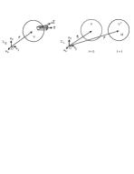
Figure 2: Euler frame $\Sigma_{E}$ (left): observe the mass flow out of a fixed volume $V$; Lagrange frame $\Sigma_{L}$ (right): follow a mass element $M$

In the Euler frame $\Sigma_{E}$ we consider a Cartesian coordinate system with origin $O$ and unit vectors ${\bf e}_{x}$, ${\bf e}_{y}$, ${\bf e}_{z}$ in $x$-, $y$-, $z$-directions. We observe the density $\rho({\bf r},t)$ [ g cm^-3 ], gas pressure $p({\bf r},t)$ [ dyn cm^-2 ], and temperature $T({\bf r},t)$ [ K ] of plasma flowing out of a fixed volume $V$ with velocity ${\bf v}({\bf r},t)$ [ cm s^-1 ] (Fig. 2). ${\bf r}$ is the radius vector with components $(x,y,z)$, and $t$ is the time. Let d${\bf A}$ be a directed surface element of $V$. Then the amount of matter flowing out of $V$ across its surface per unit time (Fig. 2) is

$$\oint\rho{\bf v}\cdot{\mathrm{d}}{\bf A}=\int\limits_{V}\nabla\cdot\rho{\bf v}\ {\mathrm{d}}V\ \ \ ,$$ (1)

where the equal sign is due to Gauss’s theorem. The amount of matter missing per unit time from volume $V$ is given by

$$-{\partial\over{\partial t}}\int\limits_{V}\rho{\mathrm{d}}V=-\int\limits_{V}{\partial\rho\over{\partial t}}\ {\mathrm{d}}V\ \ \ ,$$ (2)

where the equal sign is due to the fact that $V$ does not depend on time. Equating Eqs. (1), (2), and because $V$ is arbitrary one finds the continuity equation:

$${\partial\rho\over{\partial t}}+\nabla\cdot\rho{\bf v}=0\ \ \ .$$ (3)

2.2 Lagrange Frame

In a Lagrange frame $\Sigma_{L}$ we monitor the mass element $M$ (Fig. 2) initially contained in $V$ (at time $t=0$ and position ${\bf r}={\bf a}$), which at a later time $t$ is in volume $V^{\prime}$ at radius vector ${\bf r}({\bf a},t)=\left(x({\bf a},t),y({\bf a},t),z({\bf a},t)\right)$. Vector ${\bf a}$ uniquely identifies a mass element at the initial time $t=0$. We consider physical variables such as $\rho$ on an (x,t)-plane, on which the position of the mass element $M$ describes a path $x(t)$, where $x(t=0)=a$, so that $\rho=\rho(x(t),t)$. The rate of change of $\rho$ along that path can be pictured as the sum of the incremental variations of $\rho$ in $t$- and $x$-directions,

$${{\mathrm{d}}\rho\over{{\mathrm{d}}t}}\equiv\left({\partial\rho\over{\partial t}}\right)_{a}=\left({\partial\rho\over{\partial t}}\right)_{x}+\left({\partial\rho\over{\partial x}}\right)_{t}{{\mathrm{d}}x(t)\over{{\mathrm{d}}t}}=\left({\partial\rho\over{\partial t}}\right)_{x}+{\mathrm{v}}_{x}\left({\partial\rho\over{\partial x}}\right)_{t}\ \ \ ,$$ (4)

where the sign ($\equiv$) means equal by definition and

$${\mathrm{v}}_{x}={{\mathrm{d}}x(t)\over{\mathrm{d}}t}\ \ \$$ (5)

is the velocity of the mass element in $x$-direction. The time derivative ${\mathrm{d}}/{\mathrm{d}}t\equiv\left({\partial/{\partial t}}\right)_{a}$ in the Lagrange frame is the so called substantial derivative, sometimes also called material or total derivative. It describes the time-dependence of a physical quantity in a moving mass element. In three dimensions, and for any physical function $h$ (such as $\rho$, $p$, $T$, etc.), the substantial derivative is analogously given by

$${{\mathrm{d}}h\over{\mathrm{d}}t}={\partial h\over\partial t}+{\bf v}\cdot\nabla h\ \ \ .$$ (6)

2.3 Equation of Motion

In the Lagrange frame $\Sigma_{L}$, according to Newton’s third law the inertial force (= mass ${\mathrm{d}}M$ times acceleration ${\mathrm{d}}{\bf v}/{\mathrm{d}}t$) is balanced by the forces acting on the mass element,

$$\int\limits_{M}{{\mathrm{d}}{\bf v}\over{\mathrm{d}}t}\ {\mathrm{d}}M=\int\limits_{V}\rho{{\mathrm{d}}{\bf v}\over{{\mathrm{d}}t}}\ {\mathrm{d}}V=\int\limits_{V}{\bf f}\ {\mathrm{d}}V-\int\limits_{V}\nabla p\ {\mathrm{d}}V\ \ \ .$$ (7)

Here the acting forces consist of a volume force density ${\bf f}$ [ dyn cm^-3 ] and a pressure force. In stellar atmospheres the volume force density is due to gravity,

$${\bf f}=-{G\ M_{\star}\ \rho\over r^{2}}\ {\bf e}_{r}=-\rho\ g\ {\bf e}_{r}\ \ \ ,$$ (8)

where ${\bf e}_{r}$ is the unit vector in radial direction, $M_{\star}$ the stellar mass, $G=6.674\times 10^{-8}$ cm³ g^-1 s^-2 the gravitational constant, and $r$ the radial distance from the center of the star. As the extent $\Delta r$ of stellar atmospheres is often small ($\Delta r\ll r$), we can replace $GM_{\star}/r^{2}$ by a constant gravitational acceleration $g$, e.g. $g=2.74\times 10^{4}$ cm s^-2 for the solar atmosphere. Using Eqs. (6), (7), and (8), and noting that the volume of the mass element is arbitrary, we obtain the equation of motion

$$\rho\left({\partial{\bf v}\over{\partial t}}+{\bf v}\cdot\nabla{\bf v}\right)=-\nabla p-\rho g\ {\bf e}_{r}\ \ \ .$$ (9)

In this equation we have neglected viscosity and radiation pressure. It can be shown that both are unimportant in the atmospheres of typical late-type stars (i.e., stars of spectral type beyond late A).

2.4 Energy Equation

It is convenient to picture the moving mass element as enclosed by a wall and to carefully monitor the energy flowing through that wall. A powerful book-keeping quantity for this is the specific (i.e., per unit mass) entropy $S$ [ erg g^-1 K^-1 ]. If the walls are impermeable, energy conservation just means $S$ = constant in $\Sigma_{L}$. This can be written with Eq. (6)

$${{\mathrm{d}}S\over{\mathrm{d}}t}={\partial S\over\partial t}+{\bf v}\cdot\nabla S=0\ \ \ .$$ (10)

In atmospheric regions close to the star (in photospheres and most of the chromospheres) only two processes by which mass elements gain energy are important, radiation and Joule heating. In coronae and some chromospheric regions one has steep temperature gradients and sometimes large velocity gradients. Here thermal conduction and viscosity are other important heating (or energy loss) mechanisms. One thus has the relation

$${{\mathrm{d}}S\over{\mathrm{d}}t}={\partial S\over\partial t}+{\bf v}\cdot\nabla S=\left.{{\mathrm{d}}S\over{\mathrm{d}}t}\right|_{\mathrm{ext}}={\Phi_{\mathrm{R}}\over\rho T}+{\Phi_{\mathrm{J}}\over\rho T}+{\Phi_{\mathrm{C}}\over\rho T}+{\Phi_{\mathrm{V}}\over\rho T}\ \ \ ,$$ (11)

called entropy conservation equation. Here $\left.{\mathrm{d}}S/{\mathrm{d}}t\right|_{\mathrm{ext}}$ [ erg g^-1 K^-1 s^-1 ] is the heating function resulting from external heating by radiative, Joule, thermal conductive, and viscous heating, where $\Phi_{\mathrm{R}}$, $\Phi_{\mathrm{C}}$, and $\Phi_{\mathrm{V}}$ [ erg cm^-3 s^-1 ] are the net radiative, thermal conductive, and viscous heating rates, respectively. These functions will be discussed below. Joule heating, $\Phi_{\mathrm{J}}$, will not be considered here, although magnetic fields and associated heating (magnetohydrodynamics, MHD) are important at least in some parts of stellar chromospheres, as discussed above.

2.5 Atmospheric Gas Composition

Stellar atmospheres consist of ideal gases, which are described by the universal gas law

$$p=\sum_{i}n_{i}kT=\rho{\Re T\over\mu}\ \ \ ,$$ (12)

where $k=1.3807\times 10^{-16}$ erg K^-1 is the Boltzmann constant, $\mu$ [ g mol^-1 ] the mean molecular weight, and $\Re=8.3145\times 10^{7}$ erg K^-1 mol^-1 the universal gas constant. $n_{i}$ are the number densities [ cm^-3 ] of the different types of particles $i$ (atoms, ions, and electrons). With a given mixture of chemical elements in the stellar gas the mean molecular weight can be computed as a function $\mu=\mu(T,p)$. For solar type neutral gas $\mu\approx 1.24$, while for fully ionized gas $\mu\approx 0.60$.

2.6 Basic Elements of Thermodynamics

In many applications in stellar photospheres, chromospheres, and coronae it is sufficient to consider atmospheric gases that are either neutral or fully ionized. Under these conditions the thermodynamic relations are particularly simple. The specific internal energy $E_{s}$ [ erg g^-1 ] is given by

$$E_{s}=c_{v}T\ \ \ ,$$ (13)

where $c_{v}$ [ erg g^-1 K^-1 ] is the specific heat per unit mass for constant volume, given by

$$c_{v}={1\over\gamma-1}{\Re\over\mu}\ \ \ ,$$ (14)

and $\gamma=c_{p}/c_{v}$ is the ratio of specific heats, which is constant ($\gamma=5/3$) for either neutral or fully ionized gases. With the specific volume $V_{s}$ [ cm³ g^-1 ],

$$V_{s}={1\over\rho}\ \ \ ,$$ (15)

and the fundamental laws of thermodynamics we obtain

$$T\ {\mathrm{d}}S={\mathrm{d}}E_{s}+p\ {\mathrm{d}}V_{s}={\mathrm{d}}E_{s}-{p\over\rho^{2}}\ {\mathrm{d}}\rho\ \ \ .$$ (16)

From these equations the relationships between the thermodynamical variables $S$, $E_{s}$, $T$, $p$, and $\rho$ can be computed. Specification of two of these allows to determine the remaining variables.

2.7 Conservation Equations

It is often convenient to write the hydrodynamic equations in conservation form, in terms of conserved quantities $f$ (mass, momentum, energy) and associated fluxes ${\bf F}$ (mass flux, momentum flux, energy flux):

$${\partial f\over\partial t}=-\nabla\cdot{\bf F}+C\ \ \ ,$$ (17)

where $C$ is a source term.

a. Conservation of mass

The continuity equation (3) is already in conservation form:

$${\partial\rho\over\partial t}=-\nabla\cdot\rho{\bf v}\ \ \ .$$ (18)

b. Conservation of momentum

From Eqs. (3) and (9) one obtains

$${\partial\rho{\bf v}\over\partial t}=\rho{\partial{\bf v}\over\partial t}+{\bf v}{\partial\rho\over\partial t}=-\rho{\bf v}\cdot\nabla{\bf v}-{\bf v}\nabla\cdot\rho{\bf v}-\nabla p-\rho g{\bf e}_{r}\ \ \ ,$$ (19)

which can be written

$${\partial\rho{\bf v}\over{\partial t}}=-\nabla\cdot\left(\rho{\bf v}{\bf v}+p{\overline{\overline{U}}}\right)-\rho g{\bf e}_{r}\ \ \ .$$ (20)

Here ${\bf v}{\bf v}$ is a dyad (e.g., (Spiegel, 1969; Morse and Feshbach, 1953)), and

$${\overline{\overline{U}}}={\bf e}_{x}{\bf e}_{x}+{\bf e}_{y}{\bf e}_{y}+{\bf e}_{z}{\bf e}_{z}\ \ \ ,$$ (21)

is a unit dyad.

c. Conservation of energy

There are three types of energy densities [ erg cm^-3 ] for gas elements in nonmagnetic stellar atmospheres:

$\rho E_{s}\ \$ internal energy (energy of microscopic undirected motion of atoms and ions),

${1\over 2}\rho{\mathrm{v}}^{2}\$ kinetic energy (directed motion of the entire gas element),

$\rho\phi\ \$ potential energy (gas element in the gravitational field).

The gravitational potential is given by

$$\phi\equiv-{GM_{\star}\over r}\ \ \ .$$ (22)

With this and Eq. (8) the volume force density can be written

$${\bf f}=-\rho g{\bf e}_{r}=-\rho{GM_{\star}\over{r^{2}}}{\bf e}_{r}=-\rho\nabla\phi\ \ \ .$$ (23)

The time derivative of the total energy density can be written as a sum of four terms

$${\partial\over\partial t}\left({1\over 2}\rho{\mathrm{v}}^{2}+\rho E_{s}+\rho\phi\right)={1\over 2}{\mathrm{v}}^{2}{\partial\rho\over\partial t}+\rho{\bf v}\cdot{\partial{\bf v}\over\partial t}+{\partial\rho E_{s}\over\partial t}+{\partial\rho\phi\over\partial t}\ \ \ .$$ (24)

Modifying the terms on the RHS using Eqs. (3), (9), (11), (16), and (23), one obtains the energy conservation equation:

$${\partial\over\partial t}\left({1\over 2}\rho{\mathrm{v}}^{2}+\rho E_{s}+\rho\phi\right)=-\nabla\cdot\rho{\bf v}\left({1\over 2}{\mathrm{v}}^{2}+E_{s}+{p\over\rho}+\phi\right)+\rho T\left.{{\mathrm{d}}S\over{\mathrm{d}}t}\right|_{\mathrm{ext}}\ \ \$$

$$=-\nabla\cdot\rho{\bf v}\left({1\over 2}{\mathrm{v}}^{2}+E_{s}+{p\over\rho}+\phi\right)+\Phi_{\mathrm{R}}+\Phi_{\mathrm{J}}+\Phi_{\mathrm{C}}+\Phi_{\mathrm{V}}\ \ \ .$$ (25)

It is seen that there are three energy flux components [ erg cm^-2 s^-1 ]:

$\rho{\bf v}{1\over 2}{\mathrm{v}}^{2}\ \$ kinetic energy flux,

$\rho{\bf v}\left(E_{s}+p/\rho\right)\ \$ enthalpy flux,

$\rho{\bf v}\phi\ \$ potential energy flux.

2.8 Heating by Viscosity and Thermal Conductivity

The particle transport processes which occur in the presence of velocity and temperature gradients contribute to the local heating.

The thermal conductive heating rate $\Phi_{\mathrm{C}}$ [ erg cm^-3 s^-1 ] is given by

$$\Phi_{\mathrm{C}}={{\mathrm{d}}\over{\mathrm{d}}x}\kappa_{th}{{\mathrm{d}}T\over{\mathrm{d}}x}\ \ \ .$$ (26)

The viscous heating rate $\Phi_{\mathrm{V}}$ [ erg cm^-3 s^-1 ] is

$$\Phi_{\mathrm{V}}=\eta_{vis}\left({{\mathrm{d}}v\over{\mathrm{d}}x}\right)^{2}\ \ \ .$$ (27)

The coefficients of thermal conductivity $\kappa_{th}$ and viscosity $\eta_{vis}$ are functions of $T$ and $p$.

3 Elementary Radiation Theory

Using the three time-dependent hydrodynamic equations (18), (20), and (25) together with the ideal gas law Eq. (12), the thermodynamic relations and functions such as $\mu(T,p)$, $\kappa_{th}(T,p)$ and $\eta_{vis}(T,p)$, one would be able to compute the dynamics of stellar chromospheres, except that radiation is critically important. For this reason we now give a short review of the basic equations of radiation theory and derive the radiative heating rate. For further reading we suggest in particular (Mihalas, 1978; Rutten, 2003), but also (Stix, 2002; Seaquist, 2003), and for looking up equations and atomic data (Allen, 1973; Cox, 2000).

3.1 Basic Radiation Quantities

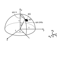
Figure 3: Left: Solid angle. Right: Intensity

a. Solid angle

Consider an orthogonal Cartesian coordinate system $(x,y,z)$. Let the latitude angle $\vartheta$ and azimuth angle $\varphi$ be defined as seen in Fig. 3, left. The solid angle is a surface element on a sphere with unit radius

$${\mathrm{d}}\Omega\equiv\sin\vartheta\ {\mathrm{d}}\vartheta\ {\mathrm{d}}\varphi\ \ \ ,$$ (28)

and has the dimension [ sr ] (for steradian).

b. Intensity

The intensity is the basic quantity of radiation theory. Consider the energy $\Delta E$ of all photons that flow through a window of area $\Delta A$ in normal direction ${\bf e}_{n}$ into the solid angle $\Delta\Omega$ per time interval $\Delta t$ and frequency interval $\Delta\nu$ (Fig. 3, right). Assume that ${\bf r}$ is the radius vector that points from the origin $O$ of a coordinate system (with unit vectors ${\bf e}_{x}$, ${\bf e}_{y}$, ${\bf e}_{z}$) to the location of the area $\Delta{\bf A}$. Then the monochromatic intensity $I_{\nu}$, also called specific intensity, is given by

$$I_{\nu}\left({\bf r},{\bf e}_{n},t\right)\equiv\lim{\Delta E\over{\Delta A\ \Delta t\ \Delta\Omega\ \Delta\nu}}\ \ \ .$$ (29)

The limit is taken for $\Delta A,\Delta t,\Delta\Omega,\Delta\nu\rightarrow 0$. $I_{\nu}$ has the dimension [ erg cm^-2 s^-1 sr^-1 Hz^-1 ] = 10^-3 [ W m^-2 sr^-1 Hz^-1 ]. Recall that 1 J = 1 Ws = 1 Nm = 1 kg m² s^-2 = 10⁷ erg.

c. Mean intensity

The mean intensity is the specific intensity averaged over all angles,

$$J_{\nu}\left({\bf r},t\right)={1\over{4\pi}}\oint I_{\nu}\left({\bf r},{\bf e}_{n},t\right)\ {\mathrm{d}}\Omega={1\over{4\pi}}{\int\limits_{0}^{\pi}}{\int\limits_{0}^{2\pi}}I_{\nu}\ \sin\vartheta\ {\mathrm{d}}\vartheta\ {\mathrm{d}}\varphi\ \ \ .$$ (30)

In most cases there is no dependence of $I_{\nu}$ on $\varphi$, and with the angle cosine

$$\mu\equiv\cos\vartheta\ \ \$$ (31)

the mean intensity can be written

$$J_{\nu}\left({\bf r},t\right)={1\over 2}{\int\limits_{0}^{\pi}}I_{\nu}\ {\underbrace{\sin\vartheta\ {\mathrm{d}}\vartheta}_{-{\mathrm{d}}\mu}}={1\over 2}{\int\limits_{-1}^{+1}}I_{\nu}\ {\mathrm{d}}\mu\ \ \ .$$ (32)

The dimension of $J_{\nu}$, [ erg cm^-2 s^-1 sr^-1 Hz^-1 ], is the same as that of $I_{\nu}$.

d. Radiative flux

Consider a window with area $\Delta A$ and normal ${\bf e}_{n}$ (Fig. 4). Assume that from both sides photons flow in arbitrary directions ${\bf e}_{n}^{\prime}$ through $\Delta{\bf A}$. The net energy $\Delta E$ transported in ${\bf e}_{n}$ direction by all the photons flowing through $\Delta A$ per time interval $\Delta t$ and frequency band $\Delta\nu$ is the radiative flux given by

$$F_{\nu}\left({\bf r},{\bf e}_{n},t\right)\ =\lim{\Delta E\over\Delta A\ \Delta t\ \Delta\nu}\ \ \ ,$$ (33)

where the limit is taken for $\Delta A,\Delta t,\Delta\nu\rightarrow 0$. $F_{\nu}$ has the dimension [ erg cm^-2 s^-1 Hz^-1 ] and can be derived from $I_{\nu}$ by summing over all projected contributions from the individual light rays in ${\bf e}_{n}^{\prime}$ direction,

$$F_{\nu}\left({\bf r},{\bf e}_{n},t\right)=\oint I_{\nu}\left({\bf r},{\bf e}_{n}^{\prime},t\right){\bf e}_{n}^{\prime}\cdot{\bf e}_{n}\ {\mathrm{d}}\Omega^{\prime}=\int\limits_{0}^{\pi}\int\limits_{0}^{2\pi}I_{\nu}\ {\underbrace{\cos\vartheta}_{\mu}}\ {\underbrace{\sin\vartheta\ {\mathrm{d}}\vartheta}_{-{\mathrm{d}}\mu}}\ {\mathrm{d}}\varphi\ \ \ ,$$ (34)

where $\vartheta$ is measured from the ${\bf e}_{n}$ direction. Here one takes into account that photons from ${\bf e}_{n}^{\prime}$ see only a projected area $\Delta A{\bf e}_{n}^{\prime}\cdot{\bf e}_{n}$. In most cases there is no $\varphi$ dependence, and

$$F_{\nu}\left({\bf r},{\bf e}_{n},t\right)=2\pi\int\limits_{-1}^{+1}I_{\nu}\ \mu\ {\mathrm{d}}\mu\ \ \ .$$ (35)

Note that $F_{\nu}$ and $I_{\nu}$ are scalar quantities that depend on the normal vector ${\bf e}_{n}$ of the considered directed unit area. In an isotropic radiation field one has $F_{\nu}=0$.

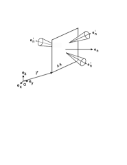
Figure 4: Radiative flux

3.2 Radiation Field, Level Populations, LTE and NLTE

Consider the interior of a cavity which has been submerged for a long time in a gas of constant temperature $T$. All time-dependent processes have quieted down, and a final state has been reached, called thermal equilibrium (TE). It is described by four important relations: the Planck function, the Boltzmann distribution, the Saha equation, and the Maxwell velocity distribution.

a. Planck function

In TE the intensity is given by the Planck function:

$$I_{\nu}=B_{\nu}\equiv{2h\nu^{3}\over c^{2}}\ {1\over{e^{h\nu/kT}-1}}\ \ \ ,$$ (36)

which upon frequency integration gives

$$I=\int I_{\nu}\ {\mathrm{d}}\nu=B\equiv\int B_{\nu}\ {\mathrm{d}}\nu={\sigma\over\pi}T^{4}\ \ \ .$$ (37)

$B$ is called the integrated Planck function. Here $h=6.626\times 10^{-27}$ erg s is the Planck constant and $\sigma=5.671\times 10^{-5}$ erg cm^-2 s^-1 K^-4 the Stefan-Boltzmann constant.

b. Boltzmann and Saha equations

Consider the energy levels of the atoms or ions of a gas (Fig. 5). The number $n_{l}$ of atoms or ions per cm³ in the bound energy level $l$ is called the population of level $l$. $n_{k}$ is the population of the continuum, i.e., the number of atoms or ions per cm³ having their electron removed by ionization. Bound levels in TE are described by the Boltzmann distribution:

$${n_{u}\over{n_{l}}}={g_{u}\over g_{l}}e^{-E_{lu}/kT}={g_{u}\over g_{l}}e^{-h\nu_{lu}/kT}\ \ \ ,$$ (38)

where $g_{i}$ are statistical weights (for hydrogen e.g. $g_{i}=2i^{2}$) and $E_{lu}$ is the energy difference between the levels (for tabulated values of these quantities see Allen (Allen, 1973; Cox, 2000)). Continuum levels in TE follow the Saha equation:

$${n_{k}\ n_{\mathrm{e}}\over{n_{l}}}={2u_{k}\over{g_{l}}}\left({2\pi m_{\mathrm{e}}kT\over{h^{2}}}\right)^{3/2}e^{-E_{l}/kT}$$ (39)

where (see (Allen, 1973; Cox, 2000)) $u_{k}$ is the partition function, $E_{l}$ the ionization energy from level $l$, $m_{\mathrm{e}}=9.1094\times 10^{-28}$ g the mass of an electron, and $n_{\mathrm{e}}$ the number of electrons per cm³. Note that the number of particles per cm³ is usually called the number density of these particles.

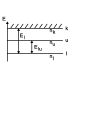
Figure 5: Energy levels

c. Maxwell distribution

In TE, atoms, ions, and electrons also obey the Maxwell velocity distribution:

$${{\mathrm{d}}n\left({\mathrm{v}}\right)\over n}=4\pi{\mathrm{v}}^{2}\left(m\over{2\pi kT}\right)^{3/2}e^{-m{\mathrm{v}}^{2}/{2kT}}\ {\mathrm{d}}{\mathrm{v}}$$ (40)

Here ${\mathrm{d}}n({\mathrm{v}})$ is the number of particles per cm³ with mass $m$ and velocities in the interval ${\mathrm{v}}$ to ${\mathrm{v}}+{\mathrm{d}}{\mathrm{v}}$, while $n$ is total number of these particles per cm³, irrespective of velocity.

TE	LTE	NLTE	Interplanetary
$I_{\nu}=B_{\nu}$	$I_{\nu}\neq B_{\nu}$	$I_{\nu}\neq B_{\nu}$	$I_{\nu}\neq B_{\nu}$
Boltzmann	Boltzmann	$\neq$Boltzmann	$\neq$Boltzmann
Saha	Saha	$\neq$Saha	$\neq$Saha
Maxwell	Maxwell	Maxwell	$\neq$Maxwell

Table 1: Various physical situations in stellar atmospheres defined by the successive break-down of relations valid in thermodynamic equilibrium. Here the symbol $\neq$ means “not equal to” or “not valid”

d. Departures from thermodynamic equilibrium: LTE, NLTE

Deep in a star one has TE (Table 1). Rising towards the surface, the first concept that breaks down is the equality of the intensity and the Planck function, while the Maxwell and Boltzmann distributions as well as the Saha equation are still valid. This is called local thermodynamic equilibrium (LTE). LTE holds roughly up to the photosphere. Rising further into the chromosphere and inner corona, both the Boltzmann distribution and the Saha equation are no longer valid. This situation is called Non-LTE (NLTE). Here the individual transition rates between the various energy levels must be considered in detail. In the low density parts of the corona the temperatures of the different particle species become unequal, and eventually in the interplanetary medium even the Maxwell distribution breaks down.

3.3 Absorption & Emission Coefficients, Source Function

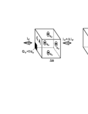
Figure 6: Left: Absorption coefficient. Right: Emission coefficient

a. Absorption coefficient

Consider in Fig. 6, left, a ray of light with intensity $I_{\nu}$, penetrating a box with surface area $\Delta A$ and thickness $\Delta s$. The absorbing or scattering atoms in the box have a number density $n$ [ cm^-3 ] and cross section $q_{\nu}$ [ cm² ]. The sum of all cross sections is $Q_{\nu}=\sum q_{\nu}$, thus:

$${\Delta I_{\nu}\over{I_{\nu}}}=-{Q_{\nu}\over{\Delta A}}=-{\sum q_{\nu}\over{\Delta A}}=-{q_{\nu}\ n\ \Delta A\ \Delta s\over\Delta A}=-\kappa_{\nu}\ \Delta s\ \ \ ,$$ (41)

where

$$\kappa_{\nu}\equiv q_{\nu}\ n\ \ \$$ (42)

is the absorption coefficient or opacity and has the dimension [ cm^-1 ]. The function ${\kappa_{\nu}(T,p)}$ is available as a program package, e.g. in the program MULTI discussed below. It is often sufficient to consider only a gray (i.e., frequency averaged) Rosseland opacity:

$$\overline{\kappa}=\left(\int\limits_{0}^{\infty}{{1\over{\kappa_{\nu}}}{dB_{\nu}\over{{\mathrm{d}}T}}{\mathrm{d}}\nu}\over{{\int\limits_{0}^{\infty}{dB_{\nu}\over{{\mathrm{d}}T}}{\mathrm{d}}\nu}}\right)^{-1}\ \ \ .$$ (43)

At photospheric and low chromospheric temperatures the gray opacity $\overline{\kappa}$ can be approximated by the $H^{-}$ contribution:

$${\overline{\kappa}\over\rho}=1.376\cdot 10^{-23}p^{0.738}T^{5}\ \mathrm{cm}^{2}\,\mathrm{g}^{-1}\ \ \ .$$ (44)

b. Emission coefficient and source function

Let the volume $\Delta V$ (Fig. 6, right) emit photons of energy $\Delta E$ in direction ${\bf e}_{n}$ into the solid angle $\Delta\Omega$ per frequency interval $\Delta\nu$ and per time interval $\Delta t$. Then

$$\eta_{\nu}\left({\bf r},{\bf e}_{n},t\right)\equiv\lim{\Delta E\over\Delta V\ \Delta t\ \Delta\Omega\ \Delta\nu}$$ (45)

is the emission coefficient with the dimension [ erg cm^-3 s^-1 sr^-1 Hz^-1 ]. Here the limit is taken for $\Delta V$, $\Delta t$, $\Delta\Omega$, $\Delta\nu\rightarrow 0$. The source function is defined as

$$S_{\nu}\left({\bf r},{\bf e}_{n},t\right)\equiv{\eta_{\nu}\left({\bf r},{\bf e}_{n},t\right)\over{\kappa_{\nu}\left({\bf r},t\right)}}\ \ \ ,$$ (46)

which has the same dimension as the intensity. In TE the amount of energy absorbed, $\Delta E_{A}$, is exactly equal to the amount of energy emitted, $\Delta E_{E}$

$$\Delta E_{A}=\ B_{\nu}\ \kappa_{\nu}\ \Delta s\ \Delta A\ \Delta t\ \Delta\Omega\ \Delta\nu\ \ ;\ \ \ \Delta E_{E}=\ \eta_{\nu}\ \Delta A\ \Delta s\ \Delta t\ \Delta\Omega\ \Delta\nu\ \ \ ,$$

which leads to Kirchhoff’s law:

$$S_{\nu}=B_{\nu}\ \ \ .$$ (47)

While in NLTE Kirchhoff’s law no longer holds, it does hold in LTE because $S_{\nu}$, as we will see below, is essentially the population ratio, $n_{u}/n_{l}$, and from our definition of LTE, this ratio, same as in TE, obeys the Boltzmann distribution.

3.4 Radiative Transfer

a. Transfer equation

Consider a gas layer in a stellar atmosphere (Fig. 7). Let ${\bf e}_{n}$ and the geometrical height $x$ point in the outward vertical direction. Consider a light ray in an arbitrary direction ${\bf e}_{n}^{\prime}$. The angle between ${\bf e}_{n}$ and ${\bf e}_{n}^{\prime}$ is $\vartheta$. Let $s$ be the geometrical distance along this light ray. From Eqs. (41), (45), and (46) we have

$${\mathrm{d}}I_{\nu}=-I_{\nu}\ \kappa_{\nu}\ {\mathrm{d}}s+\eta_{\nu}\ {\mathrm{d}}s=-\kappa_{\nu}\ \left(I_{\nu}-S_{\nu}\right)\ {\mathrm{d}}s\ \ \$$ (48)

and

$${\mathrm{d}}x=-{\mathrm{d}}s\ \cos\left(180^{\circ}-\vartheta\right)={\mathrm{d}}s\ \cos\vartheta\ =\mu\ {\mathrm{d}}s\ \ \ .$$ (49)

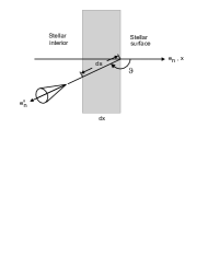
Figure 7: Transfer equation

This gives the radiative transfer equation:

$$\mu\ {{\mathrm{d}}I_{\nu}\over{\mathrm{d}}x}=-\ \kappa_{\nu}\ \left(I_{\nu}-S_{\nu}\right)\ \ \ .$$ (50)

We define the optical depth $\tau_{\nu}$:

$$\tau_{\nu}\equiv-\int\limits_{x}^{\infty}\kappa_{\nu}\ {\mathrm{d}}x\ \ \ {\rm{\ or\ }}\ \ \ {\mathrm{d}}\tau_{\nu}=-\kappa_{\nu}\ {\mathrm{d}}x\ \ \ .$$ (51)

Using Eq. (51), the transfer equation can be written in terms of the optical depth:

$$\mu\ {{\mathrm{d}}I_{\nu}\over{{\mathrm{d}}\tau_{\nu}}}=I_{\nu}-S_{\nu}\ \ \ .$$ (52)

b. Formal solution of the transfer equation

Multiplying Eq. (52) with $e^{-\tau_{\nu}/\mu}$ one finds

$${{\mathrm{d}}\left(I_{\nu}e^{-\tau_{\nu}/\mu}\right)\over{\mathrm{d}}\tau_{\nu}/\mu}=-S_{\nu}e^{-\tau_{\nu}/\mu}\ \ \ ,$$ (53)

which can be integrated between the limits $a$ and $b$:

$$I_{\nu}e^{-\tau_{\nu}/\mu}{\Bigl{|}}_{a}^{b}\Bigr{.}=-\int\limits_{a}^{b}S_{\nu}\ e^{-\tau_{\nu}^{\prime}/\mu}\ {\mathrm{d}}\tau_{\nu}^{\prime}/\mu\ \ \ .$$ (54)

Boundary conditions:

i) outer boundary: No incoming radiation from outside the star

$$I_{\nu}\left(0,\mu\right)=0\ \ ,\ \ \ \ \mu<0\ \ \ ,$$ (55)

ii) inner boundary: At the center of the star the outgoing intensity is finite

$$I_{\nu}\left(\tau_{\nu\infty},\mu\right)={\rm{finite}}\ \ ,\ \ \ \ \mu\geq 0\ \ \ .$$ (56)

Consider the case $\mu<0$, take $b=\tau_{\nu}$ and $a=0$, and multiply Eq. (54) with $e^{\tau_{\nu}/\mu}$:

$$I_{\nu}\left(\tau_{\nu},\mu\right)\ e^{-\tau_{\nu}/\mu}\ e^{\tau_{\nu}/\mu}-I_{\nu}\left(0,\mu\right)\ e^{\tau_{\nu}/\mu}=\hskip 199.16928pt$$

$$\hskip 85.35826ptI_{\nu}\left(\tau_{\nu},\mu\right)=-\int\limits_{0}^{\tau_{\nu}}S_{\nu}\ \left(\tau_{\nu}^{\prime}\right)\ e^{-\left(\tau_{\nu}^{\prime}-\tau_{\nu}\right)/\mu}\ {\mathrm{d}}\tau_{\nu}^{\prime}/\mu\ \ \ ,$$ (57)

This is valid for incoming radiation, where $\mu<0$ and $\vartheta>\pi/2$.

Now consider the other case $\mu\geq 0$, take $b=\tau_{\nu\infty}$ very large and $a=\tau_{\nu}$, and multiply Eq. (54) with $-e^{\tau_{\nu}/\mu}$:

$$-I_{\nu}\left(\tau_{\nu\infty},\mu\right)\underbrace{e^{-\tau_{\nu\infty}/\mu}}_{=0}\ e^{\tau_{\nu}/\mu}+I_{\nu}\left(\tau_{\nu},\mu\right)\ e^{-\tau_{\nu}/\mu}\ e^{\tau_{\nu}/\mu}=\hskip 142.26378pt$$

$$\hskip 113.81102ptI_{\nu}\left(\tau_{\nu},\mu\right)=\int\limits_{\tau_{\nu}}^{\infty}\ S_{\nu}\left(\tau_{\nu}^{\prime}\right)\ e^{-(\tau_{\nu}^{\prime}-\tau_{\nu})/\mu}\ {\mathrm{d}}\tau_{\nu}^{\prime}/\mu\ \ \ ,$$ (58)

This is valid for outgoing radiation, where $\mu\geq 0$ and $\vartheta<\pi/2$.

3.5 Radiative Equilibrium, Eddington Approximation

a. Radiative equilibrium

Operate with $2\pi\int\limits_{-1}^{1}{\mathrm{d}}\mu$ on Eq. (50) and use Eqs. (32), (35):

$${{\mathrm{d}}F_{\nu}\over{\mathrm{d}}x}=-4\pi\ \kappa_{\nu}\ \left(J_{\nu}-S_{\nu}\right)\ \ \ ,$$ (59)

where

$$2\pi\ \int\limits_{-1}^{+1}S_{\nu}\ {\mathrm{d}}\mu=2\pi\ S_{\nu}\int\limits_{-1}^{+1}{\mathrm{d}}\mu=4\pi\ S_{\nu}\ \ \ ,$$ (60)

if $S_{\nu}$ is assumed independent of $\mu$.

If in a plane-parallel time-independent atmosphere the energy transport is by radiation only, then $F=\int_{0}^{\infty}F_{\nu}\ {\mathrm{d}}\nu=$ const, i.e. there is a constant energy flux through all layers. This condition is called radiative equilibrium:

$${{\mathrm{d}}F\over{\mathrm{d}}x}=\int\limits_{0}^{\infty}{{\mathrm{d}}F_{\nu}\over{\mathrm{d}}x}{\mathrm{d}}\nu=-4\pi\ \int\limits_{0}^{\infty}\kappa_{\nu}\ \left(J_{\nu}-S_{\nu}\right){\mathrm{d}}\nu=0\ \ \ ,$$ (61)

which for gray opacity $\kappa_{\nu}=\overline{\kappa}$ reduces to $J=S$ as $\overline{\kappa}$ can be taken out of the integration.

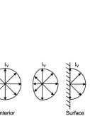
Figure 8: Isotropy of the radiation field as function of depth in the star

b. Eddington approximation

Consider the behavior of the intensity with depth (Fig. 8). If in deeper layers the intensity is approximately isotropic we get for the Eddington K-integral:

$$K_{\nu}\equiv{1\over 2}\int\limits_{-1}^{+1}I_{\nu}\mu^{2}{\mathrm{d}}\mu\simeq{1\over 2}I_{\nu}\int\limits_{-1}^{+1}\mu^{2}{\mathrm{d}}\mu={1\over 3}I_{\nu}\ \ \ .$$ (62)

Similarly for the mean intensity at the same depth we obtain

$$J_{\nu}={1\over 2}\int\limits_{-1}^{+1}I_{\nu}{\mathrm{d}}\mu\simeq{1\over 2}I_{\nu}\int\limits_{-1}^{+1}{\mathrm{d}}\mu=I_{\nu}\ \ \ .$$ (63)

We thus find the Eddington approximation:

$$K_{\nu}\simeq{1\over 3}J_{\nu}\ \ \ ,$$ (64)

which gives relatively good results even in situations where $I_{\nu}$ is fairly anisotropic.

3.6 Gray Radiative Equilibrium Atmosphere

Assume LTE, the Eddington approximation, radiative equilibrium, and gray opacity; and integrate all equations over frequency $\nu$. Then

$$S=B\ \ ,\ \ \ \ K={1\over 3}\ J\ \ ,\ \ \ \ J=S\ \ \ ,$$ (65)

from which we find with Eq. (37):

$$J=S=B={\sigma\over\pi}T^{4}\ \ \ .$$ (66)

Operate with ${1\over 2}\int\limits_{-1}^{+1}\ \mu\ {\mathrm{d}}\mu$ on the transfer eq. (52) and use Eqs. (35), (64):

$${{\mathrm{d}}K\over{\mathrm{d}}\overline{\tau}}={1\over 3}{{\mathrm{d}}J\over{{\mathrm{d}}\overline{\tau}}}=\underbrace{{1\over 2}\int\limits_{-1}^{+1}\mu\ I\ {\mathrm{d}}\mu}_{=F/4\pi}-\underbrace{{1\over 2}S\int\limits_{-1}^{+1}\mu\ {\mathrm{d}}\mu}_{=0}={F\over 4\pi}={\rm{const.}}$$ (67)

Multiply with 3 and integrate over $\overline{\tau}$:

$$J={\sigma\over\pi}\ T^{4}={3F\over 4\pi}\overline{\tau}+J(0)\ \ \ .$$ (68)

At the surface the ingoing intensity is zero, so we need to integrate only over $\mu>0$ in Eqs. (32) and (35):

$$J\left(0\right)={1\over 2}\int\limits_{0}^{1}B\left(0\right){\mathrm{d}}\mu={B\left(0\right)\over 2}\ \ \ ,\ \ \ F\left(0\right)=2\pi\int\limits_{0}^{1}B\left(0\right)\mu{\mathrm{d}}\mu=\pi B\left(0\right)\ \ \ ,$$ (69)

thus

$$J\left(0\right)={F\left(0\right)\over{2\pi}}\ \ \ .$$ (70)

Let us define:

$$F=F\left(0\right)\equiv\sigma\ T_{\mathrm{eff}}^{4}\ \ \ ,$$ (71)

where $T_{\mathrm{eff}}$ is the effective temperature. Then we find from Eqs. (68), (70), and (71) the so called gray radiative equilibrium $T(\tau)$ relation:

$$T^{4}={3\over 4}\ T_{\mathrm{eff}}^{4}\ \left(\overline{\tau}+{2\over 3}\right)\ \ \ .$$ (72)

The relation between the optical and geometrical depths is obtained from Eq. (51):

$${\mathrm{d}}\overline{\tau}=-\overline{\kappa}\ {\mathrm{d}}x\ \ \ .$$ (73)

For a plane, static (where the flow velocity ${\bf v}=0$) atmosphere we find from Eq. (9) the equation of hydrostatic equilibrium:

$${\mathrm{d}}p=-\rho\ g\ {\mathrm{d}}x\ \ \ .$$ (74)

Using for example the simple opacity law (44), it is seen that Eqs. (72), (73), and (74) can be integrated as functions of $x$. This allows to construct a static, plane, gray, radiative equilibrium atmosphere if the two quantities $T_{\mathrm{eff}}$ and $g$ as well as suitable boundary conditions are given. Together with Eq. (12), $p=\rho\Re T/\mu$, we have four equations for the four unknowns $T,p,\rho$, and $\overline{\tau}$. Such radiative equilibrium atmospheres are the starting atmosphere models for chromospheric wave calculations.

3.7 Net Radiative Heating Rate, Radiative Heating Function

The net radiative heating rate, $\Phi_{\mathrm{R}}$ [ erg cm^-3 s^-1 ], (see Eq. 11) is the negative divergence of the total radiative energy flux $F=\int_{0}^{\infty}F_{\nu}\ {\mathrm{d}}\nu$, thus in the 1D case we have

$$\Phi_{\mathrm{R}}=-{{\mathrm{d}}F\over{\mathrm{d}}x}\ \ \ .$$ (75)

Integrating Eq. (59) over $\nu$ we find from Eq. (75) the radiative heating rate

$$\Phi_{\mathrm{R}}=4\pi\int_{0}^{\infty}\kappa_{\nu}\left(J_{\nu}-S_{\nu}\right){\mathrm{d}}\nu\ \ \ ,$$ (76)

4 NLTE Thermodynamics and Radiation

As noted above (cf. Table 1), NLTE conditions prevail in the chromosphere and corona, so that in these outer stellar regions the individual transitions giving rise to lines and continua have to be considered. Chromospheres and coronae are regions where there is mechanical heating and where departures from LTE are important. Starting with a slight departure in the upper photosphere, NLTE becomes extreme in the high chromosphere and corona. It is therefore necessary to review the transition rates and outline the methods to treat the thermodynamics and radiation under NLTE conditions. General literature for this section includes (Mihalas, 1978; Rutten, 2003; Stix, 2002; Allen, 1973; Cox, 2000; Scharmer and Carlsson, 1985; Carlsson, 1992, 1995).

4.1 Transition Rates for Lines and Continua

Under NLTE conditions, there exists a well-defined kinetic temperature $T$ that is determined by the Maxwell velocity distribution, but the Boltzmann distribution and the Saha equation (Eqs. 38, 39) are no longer valid. Conservation of particles requires that the population $n_{m}$ of level $m$ obeys the time-dependent statistical rate equation

$${\partial n_{m}\over\partial t}+\nabla\cdot n_{m}{\bf v}=\sum_{j\neq m}n_{j}P_{jm}-n_{m}\sum_{j\neq m}P_{mj}\ \ \ ,$$ (77)

where $P_{ab}$ denotes the transition rates (= the number of transitions per sec) from level $a$ to level $b$. In cases where populations adjust faster than the time scale over which $n_{m}$ varies in hydrodynamic changes, the statistical equilibrium equation holds,

$$\sum_{j\neq m}n_{j}P_{jm}=\sum_{j\neq m}n_{j}(R_{jm}+C_{jm})=n_{m}\sum_{j\neq m}P_{mj}=n_{m}\sum_{j\neq m}(R_{mj}+C_{mj})\ \ \ ,$$ (78)

where $R$ denotes radiative and $C$ collisional transition rates [ cm^-3 s^-1 ]. Here $R_{\uparrow}$ is the absorption rate, $R_{\downarrow}^{\mathrm{ind}}$ the induced emission rate, $R_{\downarrow}^{\mathrm{sp}}$ the spontaneous emission rate, $C_{\uparrow}$ the collisional excitation or ionization rate, and $C_{\downarrow}$ the collisional deexcitation or recombination rate.

a. Lines

The radiative transition rates between two bound energy levels, a lower level $l$ and an upper level $u$ (Fig. 5), are

$$R_{\uparrow}=n_{l}R_{lu}=n_{l}B_{lu}\overline{J}_{lu}\ \ ,\ \ R_{\downarrow}^{\mathrm{ind}}=n_{u}B_{ul}\overline{J}_{lu}\ \ ,\ \ R_{\downarrow}^{\mathrm{sp}}=n_{u}A_{ul}\ \ ,$$ (79)

where $A_{ul}$, $B_{lu}$, and $B_{ul}$ are the Einstein coefficients (tabulated e.g. by Allen (Allen, 1973; Cox, 2000)). $\overline{J}_{lu}$ is the mean intensity $J_{\nu}$, averaged over the line. If $\ \varphi_{\nu}$ is the line profile, then

$$\overline{J}_{lu}\equiv\int_{\Delta\nu}\varphi_{\nu}J_{\nu}{\mathrm{d}}\nu\ \ \rm{with}\ \ \int_{\Delta\nu}\varphi_{\nu}{\mathrm{d}}\nu=1\ \ \ .$$ (80)

Here the frequency integrals extend over the width ${\Delta\nu}$ of the line. In the above equations we have assumed that the emission and absorption profiles of the line are identical, that is, we assume complete redistribution, CRD. The line profile is usually given by the Voigt profile (see Fig. 9)

$$\varphi_{\nu}={1\over\sqrt{\pi}\Delta\nu_{\mathrm{D}}}H(a,{\mathrm{v}})\ \ \ ,$$ (81)

where the damping parameter $a$ and the normalized frequency separation ${\mathrm{v}}$ are given by

$$a={\Gamma\over 4\pi\Delta\nu_{\mathrm{D}}}\ \ \ ,\ \ \ {\mathrm{v}}={\nu-\nu_{0}\over\Delta\nu_{\mathrm{D}}}\ \ \ .$$ (82)

Here $\nu_{0}$ is the line center frequency, $\Delta\nu_{\mathrm{D}}$ the Doppler width and $\Gamma$ the damping constant.

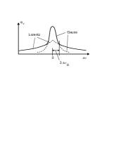
Figure 9: The Voigt spectral line profile consists of folded Gauss and Lorentz profiles.

In thermal equilibrium (TE), detailed balancing is valid, i.e. the radiation and collision processes individually balance each other,

$$R_{\uparrow}=R_{\downarrow}^{\mathrm{ind}}+R_{\downarrow}^{\mathrm{sp}}\ \ \ ,\ \ \ n_{l}B_{lu}\ B_{\nu}=n_{u}\ A_{ul}+n_{u}\ B_{ul}\ B_{\nu}\ \ \ .$$ (83)

Dividing by $n_{u}B_{ul}$, solving for $B_{\nu}$, and using Eqs. (36) and (38), one obtains

$$B_{\nu}={A_{ul}\over{B_{ul}}}{1\over{{n_{l}\over{n_{u}}}{B_{lu}\over{B_{ul}}}-1}}={A_{ul}\over{B_{ul}}}{1\over{\left({g_{l}\over{g_{u}}}e^{{h\nu_{lu}\over{kT}}}\right){B_{lu}\over{B_{ul}}}-1}}={2h\nu^{3}\over{c^{2}}}\ \ {1\over{e^{{h\nu\over{kT}}}-1}}\ \ \ ,$$ (84)

and because $T$ is arbitrary

$$A_{ul}={2h\nu^{3}\over{c^{2}}}B_{ul}\ \ \ ,$$ (85)

$$g_{l}B_{lu}=g_{u}B_{ul}\ \ \ .$$ (86)

From Eq. (79) one sees that $A_{ul}$ has the dimension [ s^-1 ], while $B_{ul}$ and $B_{lu}$ have the dimension [ cm² sr Hz erg^-1 ]. Eqs. (85) and (86) are relations between probabilities that involve only atomic parameters and do not depend on atomic level populations, they thus are also valid in NLTE. Let us introduce an absorption cross section [ cm² ]

$$\alpha_{lu}(\nu)\equiv{\pi e^{2}\over m_{\mathrm{e}}c}f_{l}\varphi_{\nu}\equiv B_{lu}{h\nu_{lu}\over 4\pi}\varphi_{\nu}\ \ \ .$$ (87)

Here $e$ is the elementary charge, $m_{\mathrm{e}}$ the electron mass, and $f_{l}$ the oscillator strength. Let us write the Boltzmann distribution (38) in the form

$${n_{u}^{\star}\over n_{l}^{\star}}={g_{u}\over g_{l}}e^{-{h\nu_{lu}\over{kT}}}\ \ \ ,$$ (88)

where $g_{i}=2i^{2}$ and populations marked by a $\star$ indicate quantities in TE or LTE. One finds

$$A_{ul}=B_{lu}{2h\nu^{3}\over{c^{2}}}{n_{l}^{\star}\over n_{u}^{\star}}e^{-{h\nu\over{kT}}}\ \ \ ,\ \ \ B_{ul}=B_{lu}{n_{l}^{\star}\over n_{u}^{\star}}e^{-{h\nu\over{kT}}}\ \ \ .$$ (89)

With this the radiative transition rates can be written

$$R_{\uparrow} = n_{l}\int_{\Delta\nu}\alpha_{lu}(\nu){4\pi\over{h\nu}}J_{\nu}{\mathrm{d}}\nu\equiv n_{l}R_{lu}\ ,$$ (90)

$$R^{\mathrm{ind}}_{\downarrow} = n_{u}{n_{l}^{\star}\over n_{u}^{\star}}\int_{\Delta\nu}\alpha_{lu}(\nu){4\pi\over{h\nu}}J_{\nu}e^{-{h\nu\over{kT}}}{\mathrm{d}}\nu\ ,$$ (91)

$$R^{\mathrm{sp}}_{\downarrow} = n_{u}{n_{l}^{\star}\over n_{u}^{\star}}\int_{\Delta\nu}\alpha_{lu}(\nu){4\pi\over{h\nu}}{2h\nu^{3}\over{c^{2}}}e^{-{h\nu\over{kT}}}{\mathrm{d}}\nu\ .$$ (92)

Defining

$$G_{ul}\equiv{g_{l}\over g_{u}}\ \ \ ,\ \ \ R_{ul}^{\dagger}\equiv\int_{\Delta\nu}\alpha_{lu}(\nu){4\pi\over{h\nu}}\left({2h\nu^{3}\over{c^{2}}}+J_{\nu}\right)e^{-{h\nu\over{kT}}}{\mathrm{d}}\nu\ \ \ ,$$ (93)

the total radiative deexitation rate is given by

$$R_{\downarrow}=R^{\mathrm{sp}}_{\downarrow}+R^{\mathrm{ind}}_{\downarrow}\equiv n_{u}R_{ul}=n_{u}\int_{\Delta\nu}\alpha_{lu}(\nu)G_{ul}{4\pi\over{h\nu}}\left({2h\nu^{3}\over{c^{2}}}+J_{\nu}\right){\mathrm{d}}\nu=n_{u}{n_{l}^{\star}\over n_{u}^{\star}}R_{ul}^{\dagger}\ \ \ .$$ (94)

For the collisional excitation and deexcitation rates [ cm^-3 s^-1 ] one has, respectively,

$$C_{\uparrow}=n_{l}\ C_{lu}=\ n_{l}\ n_{\mathrm{e}}\Omega_{lu}(T)\ \ \ ,\ \ \ C_{\downarrow}=n_{u}\ C_{ul}\ =n_{u}\ n_{\mathrm{e}}\Omega_{ul}(T)\ \ \ .$$ (95)

The $\Omega$s are called collision cross sections. In TE, because of detailed balancing, one finds

$$C_{ul}={n_{l}^{\star}\over{n_{u}}^{\star}}C_{lu}={n_{l}^{\star}\over{n_{u}}^{\star}}n_{\mathrm{e}}\Omega_{lu}(T)={g_{l}\over{g_{u}}}e^{{h\nu_{ul}\over{kT}}}n_{\mathrm{e}}\Omega_{lu}(T)\ \ \ .$$ (96)

This relation between the collision cross sections is also valid in NLTE because it involves only atomic parameters and the Maxwell velocity distribution.

b. Continua

The radiative transition rates [ cm^-3 s^-1 ] between a bound level $l$ and the continuum $k$ (Fig. 5) can be derived using similar arguments and detailed balancing in each frequency interval:

$$R_{\uparrow}=n_{l}\ R_{lk}=n_{l}\int_{\nu_{l}}^{\infty}\alpha_{l}\left(\nu\right){4\pi\over{h\nu}}J_{\nu}{\mathrm{d}}\nu\ \ \ ,$$ (97)

$$R_{\downarrow}^{\mathrm{ind}}=n_{k}{n_{l}^{\star}\over{n_{k}^{\star}}}\int_{\nu_{l}}^{\infty}\alpha_{l}\left(\nu\right){4\pi\over{h\nu}}J_{\nu}e^{-{h\nu\over{kT}}}{\mathrm{d}}\nu\ \ \ ,$$ (98)

$$R_{\downarrow}^{\mathrm{sp}}=n_{k}{n_{l}^{\star}\over{n_{k}^{\star}}}\int_{\nu_{l}}^{\infty}\alpha_{l}\left(\nu\right){4\pi\over{h\nu}}{2h\nu^{3}\over{c^{2}}}e^{-{h\nu\over{kT}}}{\mathrm{d}}\nu\ \ \ .$$ (99)

In TE and LTE the Saha equation (39) is written

$${n_{l}^{\star}\over{n_{k}^{\star}}}=n_{\mathrm{e}}\left({h^{2}\over{2\pi m_{\mathrm{e}}kT}}\right)^{3/2}{g_{l}\over{2u_{k}}}e^{{h\nu_{l}\over{kT}}}\ \ \ ,$$ (100)

where $E_{l}=h\nu_{l}$ is the energy difference between level $l$ and the continuum. $u_{k}$ in Eq. (100) is the partition function

$$u_{k}=\sum_{i=1}^{i_{\mathrm{max}}}g_{i}e^{-{h(\nu_{i}-\nu_{1})\over{kT}}}\ \ \ ,$$ (101)

where the summation is carried out over the $i_{\mathrm{max}}$ bound levels of the next higher ionization stage. It can be shown that Eqs. (98) and (99) are also valid in NLTE. Defining

$$G_{kl}\equiv{n_{l}^{\star}\over n_{k}^{\star}}e^{-{h\nu\over kT}}\ \ \ ,\ \ \ R_{kl}^{\dagger}\equiv\int_{\nu_{l}}^{\infty}\alpha_{l}(\nu){4\pi\over{h\nu}}\left({2h\nu^{3}\over{c^{2}}}+J_{\nu}\right)e^{-{h\nu\over{kT}}}{\mathrm{d}}\nu\ \ \ ,$$ (102)

the total radiative recombination rate is given by

$$R_{\downarrow}=R_{\downarrow}^{\mathrm{sp}}+R_{\downarrow}^{\mathrm{ind}}\equiv n_{k}R_{kl}=n_{k}\int_{\nu_{l}}^{\infty}\!\alpha_{l}\left(\nu\right)G_{kl}{4\pi\over{h\nu}}\!\left({2h\nu^{3}\over{c^{2}}}+J_{\nu}\right)\!{\mathrm{d}}\nu=n_{k}{n_{l}^{\star}\over n_{k}^{\star}}R_{kl}^{\dagger}\ \ \ .$$ (103)

For the collisional ionization and recombination rates [ cm^-3 s^-1 ] one finds similarly

$$C_{\uparrow}=n_{l}C_{lk}=n_{l}n_{\mathrm{e}}\Omega_{lk}\left(T\right)\ \ \ ,\ \ \ C_{\downarrow}=n_{k}C_{kl}=n_{k}n_{\mathrm{e}}^{2}\overline{\Omega}_{kl}\left(T\right)\equiv n_{k}n_{\mathrm{e}}\Omega_{kl}\left(T,n_{\mathrm{e}}\right)\ \ \ .$$ (104)

In TE, because of detailed balancing, one has

$$C_{\downarrow}=n_{k}C_{kl}=n_{k}{n_{l}^{\star}\over{n_{k}^{\star}}}C_{lk}=n_{k}{n_{l}^{\star}\over{n_{k}^{\star}}}n_{\mathrm{e}}\Omega_{lk}\left(T\right)\ \ \ ,$$ (105)

with ${n_{l}^{\star}/{n_{k}^{\star}}}$ given by Eq. (100). This relation is also valid in NLTE. Partition functions, absorption and collision cross sections ($\alpha$’s and $\Omega$’s) can be found in Allen (Allen, 1973; Cox, 2000) and references cited there.

4.2 Line and Continuum Source Functions

We now consider the transfer of radiation through a stellar gas. After Eq. (46) the source function is defined as the ratio of the emission and absorption coefficients.

a. Lines

From Eqs. (45) and (79), noting that the dimension of the transition rates is [ cm^-3 s^-1 ], one finds for the line emission coefficient [ erg cm^-3 s^-1 sr^-1 Hz^-1 ]

$$\eta_{\nu}^{\mathrm{line}}={\partial R_{\downarrow}^{\mathrm{sp}}\over{\partial\nu}}{h\nu\over{4\pi}}=n_{u}A_{ul}{h\nu\over{4\pi}}\varphi_{\nu}={2h\nu^{3}\over c^{2}}\alpha_{lu}(\nu)n_{u}G_{ul}.$$ (106)

Similarly from Eqs. (41) and (79), noting that

$${\Delta I_{\nu}\over{\Delta s}}=-I_{\nu}\kappa_{\nu}=-{\partial\left(R_{\uparrow}-R_{\downarrow}^{\mathrm{ind}}\right)\over{\partial\nu}}{h\nu\over{4\pi}}\ \ \ ,$$ (107)

the line opacity [ cm^-1 ] is given by

$$\kappa_{\nu}^{\mathrm{line}}=\left(n_{l}B_{lu}-n_{u}B_{ul}\right){h\nu\over{4\pi}}\varphi_{\nu}=n_{l}B_{lu}\left(1-{n_{u}g_{l}\over{n_{l}g_{u}}}\right){h\nu\over{4\pi}}\varphi_{\nu}=\alpha_{lu}(\nu)(n_{l}-n_{u}G_{ul})\ .$$ (108)

The absorption coefficient is defined for a total intensity change (which results from absorption minus induced emission). The line source function (see Eq. (46)) is

$$S_{lu}^{\mathrm{line}}\equiv{\eta_{\nu}^{\mathrm{line}}\over{\kappa_{\nu}^{\mathrm{line}}}}={n_{u}A_{ul}\over{n_{l}B_{lu}-n_{u}B_{ul}}}={2h\nu^{3}\over{c^{2}}}{1\over{n_{l}g_{u}\over n_{u}g_{l}}-1}={2h\nu^{3}\over{c^{2}}}{1\over{b_{l}\over b_{u}}e^{{h\nu\over kT}}-1}\ \ \ ,$$ (109)

where we have used the Boltzmann distribution. The departure from LTE coefficient $b_{l}$ is defined by

$$b_{l}\equiv{n_{l}\over n_{l}^{\star}}{n_{k}^{\star}\over n_{k}}\ \ \ .$$ (110)

Note that always $b_{k}=1$. It is seen that in LTE

$$S_{lu}^{\mathrm{line}}=B_{\nu},\ \ \ {\rm with}\ \ \ b_{l}=b_{u}=1\ \ \ .$$ (111)

In deriving Eqs. (106) and (108) we have assumed complete redistribution (CRD).

b. Continua

From Eqs. (45) and (99) we have similarly a continuum emission coefficient [ erg cm^-3 s^-1 sr^-1 Hz^-1 ]

$$\eta_{\nu}^{\mathrm{cont}}={\partial R_{\downarrow}^{\mathrm{sp}}\over{\partial\nu}}{h\nu\over{4\pi}}=n_{k}{n_{l}^{\star}\over{n_{k}^{\star}}}\alpha_{l}\left(\nu\right){2h\nu^{3}\over{c^{2}}}e^{-{h\nu\over{kT}}}={2h\nu^{3}\over c^{2}}\alpha_{l}(\nu)n_{k}G_{kl}\ \ \ .$$ (112)

Also, using Eqs. (97), (98), and (107), we obtain the continuum opacity [ cm^-1 ]

$$\kappa_{\nu}^{\mathrm{cont}}=\alpha_{l}\left(\nu\right)\left(n_{l}-n_{k}{n_{l}^{\star}\over{n_{k}^{\star}}}e^{-{h\nu\over{kT}}}\right)=\alpha_{l}(\nu)(n_{l}-n_{k}G_{kl})\ \ \ .$$ (113)

The continuum source function is then given by

$$S_{\nu}^{\mathrm{cont}}={\eta_{\nu}^{\mathrm{cont}}\over\kappa_{\nu}^{\mathrm{cont}}}={2h\nu^{3}\over c^{2}}{1\over{n_{l}\over n_{l}^{\star}}{n_{k}^{\star}\over n_{k}}e^{{h\nu\over kT}}-1}={2h\nu^{3}\over{c^{2}}}{1\over b_{l}e^{{h\nu\over kT}}-1}\ \ \ .$$ (114)

Note that in LTE

$$S_{\nu}^{\mathrm{cont}}=B_{\nu},\ \ \ {\rm with}\ \ \ b_{l}=1\ \ \ .$$ (115)

Eqs. (111) and (115) show the validity of Kirchhoff’s law (47) in LTE, as stated already above. Taking the source function equal to the Planck function is used as primary definition of LTE in some texts. For us here, the equality of the source and Planck functions (Eqs. (111) and (115)) is the result of the way by which we defined LTE.

4.3 Computation of the LTE and NLTE Level Populations

Suppose the temperature $T$ and gas pressure $p$ are given along with the chemical element abundance of the stellar gas. How can the number densities and level populations of the different atoms and ions be computed? Let

$$n_{r,s,i}\ \ \ ,\ \ \ n_{s,i}=\sum_{r=1}^{r_{\mathrm{max}}}n_{r,s,i}\ \ \ ,\ \ \ n_{i}=\sum_{s=1}^{s_{\mathrm{max}}}n_{s,i}\ \ \ ,$$ (116)

be the number density [ cm^-3 ] of particles in energy level $r$ and ionization stage $s$ of element $i$, the number density of particles of element $i$ in ionization stage $s$, and the total number density of particles of element $i$, respectively. Here $r=1,\cdots,r_{\mathrm{max}}$, where $r_{\mathrm{max}}$ is the number of bound levels, and $s=1,\cdots,s_{\mathrm{max}}$, where $s_{\mathrm{max}}$ is the number of ionization stages.

a. LTE populations

We first assume LTE. In this case the Boltzmann distributions and Saha equations are valid. Summing Eq. (38) over the bound levels $r$ we obtain the Boltzmann distributions with the partition functions

$${n_{r,s,i}\over n_{s,i}}={g_{r,s,i}\over u_{s,i}}\ e^{-{E_{r,s,i}\over kT}}\ \ \ ,\ \ \ u_{s,i}=\sum_{r=1}^{r_{\mathrm{max}}}g_{r,s,i}\ e^{-{(E_{r,s,i}-E_{1,s,i})\over kT}}\ \ \ .$$ (117)

Similarly summing Eq. (39) over all bound levels $l$ we find the Saha equations

$${n_{s+1,i}\over n_{s,i}}={1\over n_{\mathrm{e}}}{u_{s+1,i}\over u_{s,i}}\left({2\pi m_{\mathrm{e}}kT\over h^{2}}\right)^{3/2}\ e^{-{E_{s-1,i}-E_{s,i}\over kT}}\ \ \ .$$ (118)

One now proceeds as follows: 1. estimate $n_{\mathrm{e}}$. 2. Compute the element densities $n_{i}=\left({p/kT}-n_{\mathrm{e}}\right){A_{i}/\sum_{j}A_{j}}$. 3. Compute the $n_{s,i}$; for this we have $s_{\mathrm{max}}-1$ Eqs. (118) and the third of the Eqs. (116). Similarly compute $n_{r,s,i}$ using the $r_{\mathrm{max}}$ Eqs. (117). 4. Evaluate the new electron density $n_{\mathrm{e}}$ using the equation of charge conservation

$$n_{\mathrm{e}}=\sum_{i}\sum_{s=2}^{s_{\mathrm{max}}}s\ n_{s,i}\ \ \ .$$ (119)

Going back to step 1, we could iteratively improve $n_{\mathrm{e}}$ until a converged solution is obtained. One actually uses the much faster Newton-Raphson method by writing Eq. (119) as $f(n_{\mathrm{e}})=0$. If the true solution is written $n_{\mathrm{e}}=n_{\mathrm{e}}^{0}+\delta n_{\mathrm{e}}$, where $n_{\mathrm{e}}^{0}$ is an estimate, we have $f(n_{\mathrm{e}}^{0})+{{\mathrm{d}}f\over{\mathrm{d}}n_{\mathrm{e}}}\delta n_{\mathrm{e}}=0$. The derivative can be evaluated analytically. Solving for $\delta n_{\mathrm{e}}=-f(n_{\mathrm{e}}^{0})/{{\mathrm{d}}f\over{\mathrm{d}}n_{\mathrm{e}}}$ we get a new estimate $n_{\mathrm{e}}^{0}+\delta n_{\mathrm{e}}$, etc. This Newton-Raphson iteration converges very fast if the initial estimate $n_{\mathrm{e}}^{0}$ is reasonable.

b. NLTE populations

In NLTE the situation is different. Here not only the Boltzmann distributions and Saha equations are no longer valid, but also the mean intensities $J_{\nu}$ are unknown. Of the different methods to solve the problem we discuss only the complete linearization method. A computer code for this method, MULTI (Scharmer and Carlsson (1985), Carlsson (1986), Carlsson (1992)) is available (Carlsson, 1995) and widely used in the astrophysical community.

Here one also has a given temperature $T$- and pressure $p$-distribution. One starts by selecting an electron density $n_{\mathrm{e}}$-distribution and assuming level populations $n_{i}$. Then the radiation fields $J_{\nu}$ and the statistical rate equations are computed, which leads to improved $n_{i}$. In a Newton-Raphson scheme a system of equations, with a matrix ${\buildrel=\over{W}}$ operating on the vector of variations {$\delta n_{i}$} being equal to an error vector {$E_{i}$}, is inverted and the new estimates $n_{i}+\delta n_{i}$ evaluated. After convergence of this iteration the $n_{\mathrm{e}}$-distribution is modified until the given $p$-distribution is obtained. Note that physical vectors are directed quantities in space, mathematical vectors are simply arrays denoted by curly brackets { }.

Assume that for the $n^{\mathrm{th}}$ step of the iteration scheme we have the populations $n_{i}^{\left(n\right)}$ and the transition processes $P_{ij}^{\left(n\right)}$ and seek small corrections $\delta n_{i}$ and $\delta P_{ij}$. From Eq. (78), written for level $i$, with the total number of levels $N_{L}=N+1$, we have

$$\left(n_{i}^{\left(n\right)}+\delta n_{i}^{\left(n\right)}\right)\sum\limits_{j\neq i}^{N_{L}}\left(P_{ij}^{\left(n\right)}+\delta P_{ij}^{\left(n\right)}\right)-\sum\limits_{j\neq i}^{N_{L}}\left(n_{j}^{\left(n\right)}+\delta n_{j}^{\left(n\right)}\right)\left(P_{ji}^{\left(n\right)}+\delta P_{ji}^{\left(n\right)}\right)=0\ \ \ .$$ (120)

After expanding and neglecting second order terms we get

$$\delta n_{i}^{\left(n\right)}\sum\limits_{j\neq i}^{N_{L}}P_{ij}^{\left(n\right)}+n_{i}^{\left(n\right)}\sum\limits_{j\neq i}^{N_{L}}\delta P_{ij}^{\left(n\right)}-\sum\limits_{j\neq i}^{N_{L}}\delta n_{j}^{\left(n\right)}P_{ji}^{\left(n\right)}-\sum\limits_{j\neq i}^{N_{L}}n_{j}^{\left(n\right)}\delta P_{ji}^{\left(n\right)}=E_{i}^{\left(n\right)}\ \ \ ,$$ (121)

where $E_{i}^{\left(n\right)}$ represents the zeroth order terms and vanishes for the converged solution. Our aim is to write $\delta P_{ij},\delta P_{ji}$ in terms of $\delta n_{i}$, and then to solve Eq. (121) for $\delta n_{i}$. With $\delta P_{ij}=\delta R_{ij}+\delta C_{ij}$, where $\delta C_{ij}=0$ and $\delta R_{ij}^{\mathrm{sp}}=0$ because $n_{\mathrm{e}}$ and $T$ are given, we have

$$\delta P_{ij}=\delta R_{ij} = {1\over 2}\int\limits_{-1}^{+1}\int\limits_{\Delta\nu}{4\pi\over{h\nu}}\alpha_{ij}G_{ij}\delta I_{\nu\mu}{\mathrm{d}}\nu{\mathrm{d}}\mu\ \ ,\ \ i>j$$

$$= {1\over 2}\int\limits_{-1}^{+1}\int\limits_{\Delta\nu}{4\pi\over{h\nu}}\alpha_{ij}\delta I_{\nu\mu}{\mathrm{d}}\nu{\mathrm{d}}\mu\ \ ,\ \ i<j\ \ \ .$$ (122)

$\alpha_{ij}$ is given by Eq. (87) for lines, and $\alpha_{ik}=\alpha_{i}\left(\nu\right)$ from Eq. (97) for continua. The $G_{ij}$ are given by Eqs. (93) and (102), and the $\nu$-integration interval $\Delta\nu$ is either over the line width or from $\nu_{i}$ to infinity, depending on whether a line or a continuum transition is considered.

The intensities $\delta I_{\nu\mu}$ are obtained from a linearization of the radiative transfer equations, where it is important that the in- and outgoing intensities at depth $d$ originate from other points of the atmosphere than depth $d$, depending on the considered frequency. This is done using a linear system in matrix form shown in Fig. 10. With vectors $\delta{\bf n}=\{\delta n_{id}\}$, ${\bf E}=\{E_{id}\}$, where $i=1,\cdots,N_{L}$ is the energy level index and $d=1,\cdots,N_{D}$ the depth index, Eq. (121) can be written with a grand matrix ${\buildrel=\over{W}}$,

$${\buildrel=\over{W}}\ \delta{\bf n}={\bf E}\ \ \ .$$ (123)

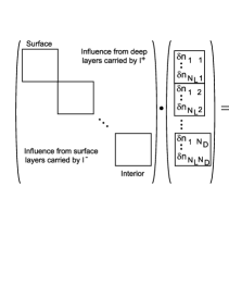
Figure 10: Matrix equation in the complete linearization method as used by Carlsson (1986)

As an example Fig. 11 shows the non-vanishing elements of the grand matrix ${\buildrel=\over{W}}$ for a 5 level + continuum Ca II calculation. The non-zero matrix elements are clustered along the main diagonal, showing that the most important radiative interactions are of intermediate range. The off-diagonal matrix elements represent the non-local contributions. This band structure permits an efficient matrix inversion.

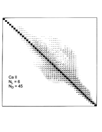
Figure 11: Grand matrix ${\buildrel=\over{W}}$ for a 5 level + continuum Ca II calculation of the solar VAL81-C model (Vernazza et al., 1981), after Carlsson (1986).

4.4 Chromospheric Radiation Loss

From the procedure discussed above the net heating rates [ erg cm^-3 s^-1 ] for lines and continua can be determined as $\Phi_{lu},\ \Phi_{l}=h\nu\left(R_{\uparrow}-R_{\downarrow}\right)$:

$$\Phi_{lu}=n_{l}4\pi\int_{\Delta\nu}\alpha_{lu}(\nu)J_{\nu}{\mathrm{d}}\nu\ -n_{u}{n_{l}^{\star}\over n_{u}^{\star}}4\pi\int_{\Delta\nu}\alpha_{lu}(\nu)\left({2h\nu^{3}\over c^{2}}+J_{\nu}\right)\ e^{-{h\nu\over kT}}{\mathrm{d}}\nu\ \ \ ,$$ (124)

$$\Phi_{l}=n_{l}4\pi\int_{\nu_{l}}^{\infty}\alpha_{l}(\nu)J_{\nu}{\mathrm{d}}\nu\ -n_{k}{n_{l}^{\star}\over n_{k}^{\star}}4\pi\int_{\nu_{l}}^{\infty}\alpha_{l}(\nu)\left({2h\nu^{3}\over c^{2}}+J_{\nu}\right)\ e^{-{h\nu\over kT}}{\mathrm{d}}\nu\ \ \ .$$ (125)

4.5 Coronal Radiation Loss

In the tenuous coronal layers the temperature is high and the density is very low. Consider the energy levels of a typical multiply ionized coronal ion with its large ionization $E_{l}$ and excitation $E_{lu}$ energies (Fig. 5). Because the photospheric radiation field $J_{\nu}$ does not provide photons with enough energy to excite a coronal ion, $R_{\uparrow}\approx 0$ and $R_{\downarrow}^{\mathrm{ind}}\approx 0$. In addition, as $n_{\mathrm{e}}$ is very small in the corona, $C_{\downarrow}\approx 0$. What remains from Eq. (78) is

$$C_{\uparrow}=R_{\downarrow}^{\mathrm{sp}}\ \ \ ,$$ (126)

which is called the thin plasma approximation. From Eqs. (99) and (104):

$$n_{1}n_{\mathrm{e}}\Omega_{1}\left(T\right)=n_{k}{n_{1}^{\star}\over n_{k}^{\star}}\int_{\nu_{1}}^{\infty}\alpha_{1}(\nu){4\pi\over h\nu}{2h\nu^{3}\over c^{2}}\ e^{-{h\nu\over kT}}{\mathrm{d}}\nu\equiv n_{k}n_{\mathrm{e}}f\left(T\right)\ \ ,$$ (127)

where we used the Saha eq. (100),

$${n_{k}^{\star}\over n_{1}^{\star}}={1\over n_{\mathrm{e}}}\left({2\pi m_{\mathrm{e}}kT\over h^{2}}\right)^{3/2}{2u_{k}\over g_{1}}e^{-{h\nu_{1}\over{kT}}}\ \ \ .$$ (128)

and collected the temperature-dependent parts in some function $f(T)$. This gives

$${n_{k}\over{n_{1}}}={\Omega_{1}\left(T\right)\over{f\left(T\right)}}\equiv g\left(T\right)\ \ \ .$$ (129)

The function $g(T)$ can be tabulated (e.g. Jain and Narain (1978)).

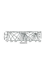
Figure 12: Ionization ratios for Fe in the thin plasma approximation valid for the corona

Note that as lower bound level we took $l=1$ because only the ground level is significantly populated. Eq. (129) states that very differently from the Saha equation (128) in LTE, which depends also on $n_{\mathrm{e}}$, the coronal ionization ratio depends only on $T$, due to the thin plasma approximation. To illustrate this dependence, Fig. 12 shows the ionization ratios $n_{s,i}/\sum_{s}n_{s,i}$ for Fe in the coronal approximation.

The coronal radiation loss due to lines is

$$-\Phi_{\mathrm{R}}=4\pi\eta-\underbrace{4\pi\kappa J}_{=0}=\sum h\nu\underbrace{n_{u}R_{u1}^{\mathrm{sp}}}_{n_{1}C_{1u}}=\sum h\nu\ n_{Ion}n_{\mathrm{e}}\Omega\left(T\right)\ \ \ ,$$ (130)

where the sum is taken over all lines. The total cooling rate includes also other processes and is given by

$$-\Phi_{\mathrm{R}}=n_{\mathrm{H}}n_{\mathrm{e}}P_{\mathrm{Rad}}\left(T\right)\ \ \ ,$$ (131)

where $P_{\mathrm{Rad}}(T)$ is a function shown in Fig. 13. Similar functions were computed by numerous authors (e.g., (Cox and Tucker, 1969; McWhirter et al., 1975; Landi and Landini, 1999)).

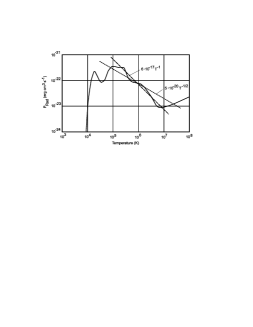
Figure 13: Radiation function $P_{\mathrm{Rad}}$ as function of temperature and various numerical fits of this function, after McWhirter et al. (1975).

The descending part is often approximated by a simple power law. A dependence $\propto T^{-1/2}$, like

$$P_{\mathrm{Rad}}\approx 5\cdot 10^{-20}T^{-1/2}$$ (132)

(after (McWhirter et al., 1975)) is particularly useful as it allows to cast the coronal energy balance in dimensionless form, thus making it possible to scale corona models from one star to another (Hammer (1984)). Please note that Eq. (131) defines only a radiative cooling function, which will ultimately cool the gas down to temperatures $T\rightarrow 0$ in the absence of heating. In reality, if $T$ becomes small enough, radiative heating must also be considered, similarly as in $\Phi_{\mathrm{R}}=4\pi\kappa\left(J-B\right)$.

5 Simulations vs. Observations

General references on the concepts discussed in this chapter include (Carlsson, 2007; Rammacher and Ulmschneider, 2003; Rammacher et al., 2005; Carlsson and Stein, 1994).

5.1 Numerical Simulations

In order to investigate the dynamics of the chromosphere theoretically, it is necessary to solve the conservation equations for mass (18), momentum (20), and energy (25) as functions of space and time for given initial and boundary values. We also need the equation of state and other thermodynamic relations necessary to close the system, Eqs. (12) – (14). Simultaneously we must calculate the ionization rates, the electron density, and the level population densities and radiative energy source and sink terms, Eqs. (124) and (125), for all important spectral lines and continua. As initial atmosphere one can e.g. use a gray radiative equilibrium atmosphere, as derived above. And as boundary conditions one typically specifies the velocity at the lower end of the computational region and allows for waves to leave the upper end with as little reflection as possible.

Ideally one would like to solve this system of partial differential equations in three dimensions (3D), in order to be able to handle the chromospheric structure. Such 3D simulations exist (e.g., Wedemeyer et al. (2004)), in some cases even including the effects of magnetic fields (Schaffenberger et al. (2006); Steiner et al. (2007); Hansteen et al. (2007)) - but unfortunately the currently available computer power does not yet permit the 3D treatment of the full problem with all the physics that is important in the chromosphere. Radiative transport must either be treated in gray LTE, or if NLTE effects are considered, they must be highly simplified; moreover the spatial resolution of fine structures such as shock waves is poor. Nevertheless, these 3D simulations provide impressive results about the structuring and dynamics of the chromosphere (see also Steiner, this volume).

Another approach restricts itself to one spatial dimension (1D), but solves the full NLTE radiation-hydrodynamics problem and calculates the variation of line profiles, which can then be compared with observations. The two most sophisticated numerical codes to deal with this problem are the one developed by M. Carlsson and R. F. Stein (briefly described in Carlsson and Stein (1994, 1995, 1997, 2002)) and the one developed by P. Ulmschneider and collaborators already since the late 1970s (e.g., (Ulmschneider et al., 1977)). We will summarize the basic working of the latter code, the most recent version of which is explained in detail in Rammacher and Ulmschneider (2003).

In order to solve a system of partial differential equations, one basically replaces differentials by finite differences that connect quantities of the known solution at the previous time level with those at the new time level, and then one solves for the latter in order to advance the solution in time.

A special feature of the Ulmschneider-Rammacher approach is that before this is done the differential equations are first transformed into their characteristic form; i.e. one takes explicitly into account that matter and hydrodynamic signals travel with speeds ${\mathrm{v}}$ and ${\mathrm{v}}\pm c$, respectively, thus defining the so-called characteristics in space-time (cf. (Landau and Lifshitz, 1959; Ulmschneider et al., 1977)). The method of characteristics has a number of advantages: It is numerically efficient (Hammer and Ulmschneider, 1978), and it makes it easy to recognize the formation of shocks (namely, when two neighboring characteristics of the same kind intersect) and to handle the jump conditions at the shock exactly - i.e., to take care of the continuity of mass, momentum, and energy fluxes across the shock, while other variables are allowed to change discontinuously. Most other methods cannot treat these discontinuities and use artificial or numerical viscosity to spread out shocks over a certain height range, and then represent each shock by a number of narrowly spaced grid points. For these reasons, characteristics methods with detailed shock handling are very fast. They are, however, best suited for 1D calculations, since the necessary bookkeeping of characteristics gets prohibitively complicated in 3D.

In this particular code, the solution is advanced in time in an iterative process. Suppose that all variables are known at some time level $t$. At the first time step these are the initial conditions to be specified. The radiative heating rates are first assumed to remain constant, and a first guess is used for the values of the hydrodynamic variables at a later time $t+\Delta t$. This allows to calculate the characteristics and the change of the variables along these characteristics, leading to improved values of the hydrodynamic variables in the next iteration. This hydrodynamic iteration converges after a few steps. After the hydrodynamic variables at the new time level are known, the population levels and radiative intensities can be calculated, providing the radiative heating rates. These are used in the next hydrodynamic iteration to further improve the hydrodynamic variables, which in turn lead to improved population levels and radiative heating rates, and so on. If the radiative terms or any other quantities are found to change too rapidly or too slowly during this process, the time step $\Delta t$ is decreased or increased accordingly.

For reasons of computing time efficiency, the radiative part is usually simplified during the simulation, and full line profiles for diagnostic purposes are calculated with codes like MULTI only at specific time steps.

A movie clip from an example calculation (Rammacher (2007)) shows how a spectrum of waves moves through the atmosphere, steepening into shocks that continue to grow, whereby occasionally larger ones catch up and merge with smaller ones. The associated emission is rather complex: Even though a major contribution comes usually from behind large shocks, because of the long-range interaction of chromospheric radiation other parts of the atmosphere can also make significant contributions, depending on the changing availability of emitters/absorbers and photons in various parts of the highly dynamic atmosphere. In the movie clip (Rammacher, 2007) this is illustrated for two wavelengths in the blue wing of Ca ii K.

5.2 Comparison with Observations

Such 1D simulations have been very successful (Rammacher and Ulmschneider (1992), Carlsson and Stein (1992, 1997)) in explaining the Ca H and K Bright Grain phenomenon, a characteristic variation of the line profiles of Ca ii H and K that arises when strong acoustic shocks traverse the mid-chromosphere.

Simulations in which the waves were injected according to photospheric velocity measurements led to the surprising result that the average temperature beyond a height of 500 km (the canonical location of the temperature minimum) did not increase, but continued to drop outward (Carlsson and Stein (1994, 1995)). The emission behind strong shocks was found to be so large that no general temperature rise was needed to generate the chromospheric emission in lines such as Ca ii H and K. There has been some debate if this low average temperature is real or caused by the neglect of high frequency waves, which are on principle not observable due to their short wavelengths (Kalkofen et al. (1999), Carlsson (2007)). The problem could also be related to the 3D character of wave propagation in the real solar chromosphere, which according to Ulmschneider et al. (2005) reduces the generation of very strong shocks by the merging of weaker ones, as commonly found in 1D models, but rather leads to a more continuous heating by a larger number of weak shocks. Moreover, the meaning of an “average” temperature becomes questionable in the presence of large temperature fluctuations (Carlsson and Stein (1995); Rammacher and Cuntz (2005)).

Acoustic shock waves have long (Biermann, 1946) been thought to be the main heating agent of outer stellar atmospheres, or at least of the nonmagnetic parts of stellar chromospheres (for a review see e.g. Ulmschneider and Musielak (2003)). This view has been challenged recently, when Fossum and Carlsson (Fossum and Carlsson, 2005a, b, 2006) used 1D simulations to interpret the fluctuations observed by the TRACE satellite in UV continua formed in the upper photosphere. They concluded that the small observed fluctuations permit only an acoustic energy flux at least an order of magnitude too small to balance the chromospheric energy losses. Wedemeyer-Böhm et al. (2007) demonstrated, however, that this is mostly due to the fact that the spatial resolution of TRACE is insufficient to resolve the fine-scaled lateral structuring found in 3D simulations. And Cuntz et al. (2007) argued that such a low acoustic energy flux would be inconsistent with theoretical calculations of sound generation (Musielak et al. (1994)) and with the excellent agreement between simulations and the measured Ca emission of the most inactive stars. Therefore, it appears that the acoustic heating theory is still valid and cannot be considered dead at this time (Mark Twain, 1897).

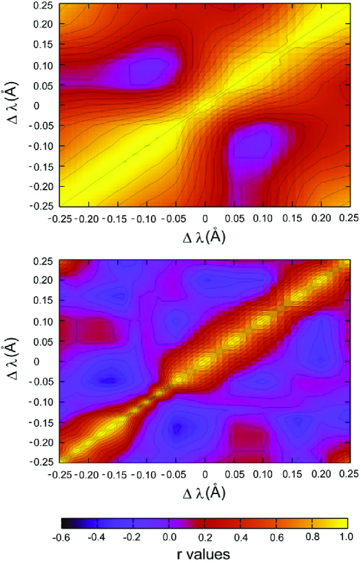
Figure 14: Ca ii H correlation matrices for VTT observations (top panel) and for a 1D model simulation using a power spectrum with total input energy flux of $5.0\times 10^{7}$ erg cm^-2 s^-1 (bottom panel); from (Rammacher et al., 2007a).

Even though 1D simulations describe reasonably well the dynamics of mostly vertically propagating strong shocks (Ca Bright Grains, as discussed above), they fail to match the overall dynamics of the solar chromosphere. If the chromosphere were dominated by upward propagating plane-parallel waves, the resulting perturbations in the Ca ii H and K lines would always start in the line wings (which are formed in the photosphere) and then move inward towards the line center (which is formed in the upper chromosphere). Observations Rammacher et al. (2007b) show that this may happen indeed, however one often sees large portions of the blue or red wing increase simultaneously. To quantify this behavior, W. Rammacher (Rammacher et al., 2007a) has introduced a diagram that may serve as a “fingerprint” of the dynamics of the chromosphere (Fig. 14). It shows the correlation $r$ of the intensity at any wavelength with the intensity at all other wavelengths in the line profile. If two parts of the atmosphere, where two different wavelengths are formed, always vary simultaneously, the correlation $r$ is 1. Obviously this must be true for the diagonal. On the other hand, if the dynamics in the two parts of the atmosphere are completely unrelated, the correlation is $r=0$; whereas $r=-1$ means total anticorrelation, i.e., one part of the atmosphere always brightens when the other darkens. Observations (upper panel in Fig. 14) show a much higher degree of intensity correlation between different parts of the atmosphere than 1D numerical simulations (lower panel). The difference to the observed fingerprint turned out to be large for all numerical simulations, irrespective of the amount of wave energy and the spectrum of wave frequencies used. (According to (Rammacher, 2005) the chromosphere depends less sensitively on the wave spectrum than on the energy flux.) Therefore, vertically propagating shock waves cannot explain the observations. Rammacher et al. (2007a) suggest that oblique shock fronts could explain the high observed correlations, because they would lead to a simultaneous brightening of deeper and higher parts of the atmosphere. Such oblique shock fronts are commonly found in 3D simulations (Wedemeyer et al. (2004); Wedemeyer-Böhm et al. (2005)); also Ulmschneider et al. (2005) argued theoretically that 3D propagation of shock waves must be important.

To summarize, the highly dynamic solar chromosphere (described in the first chapter of this paper) calls for the simultaneous solution of the radiation hydrodynamic equations under NLTE conditions (as discussed in the next three chapters). Modern computers allow their full solution in 1D, while for 3D calculations, due to the present lack of sufficient computational power, simplifications have to be made. Since 3D effects turned out to be important in the real solar chromosphere (as discussed in this chapter), we will have to take advantage of the best features of both types of calculations over the next few years and combine them with the ever improving observational capabilities in order to understand the dynamic solar chromosphere.

References

- Vernazza et al. (1981) J. E. Vernazza, E. H. Avrett, and R. Loeser, Astrophys. J. Suppl. 45, 635–725 (1981).
- Fontenla et al. (1993) J. M. Fontenla, E. H. Avrett, and R. Loeser, Astrophys. J. 406, 319–345 (1993).
- Avrett (2007) E. H. Avrett, “New Models of the Solar Chromosphere and Transition Region Determined from SUMER Observations,” in The Physics of Chromospheric Plasmas, ASP Conf. Ser. 368, edited by P. Heinzl, I. Dorotovič, and R. J. Rutten, San Francisco: ASP, 2007, pp. 81–91.
- Fontenla, et al. (2007) J. M. Fontenla,, K. S. Balasubramaniam, and J. Harder, “Chromospheric Heating and Low-chromospheric Modeling,” in The Physics of Chromospheric Plasmas, ASP Conf. Ser. 368, edited by P. Heinzl, I. Dorotovič, and R. J. Rutten, San Francisco: ASP, 2007, pp. 499–503.
- Solanki and Hammer (2002) S. K. Solanki, and R. Hammer, “The Solar Atmosphere,” in The Century of Space Science, edited by J. A. Bleeker, J. Geiss, and M. Huber, Berlin: Springer, 2002, pp. 1065–1088.
- Narain and Ulmschneider (1990) U. Narain, and P. Ulmschneider, Space Science Reviews 54, 377–445 (1990).
- Narain and Ulmschneider (1996) U. Narain, and P. Ulmschneider, Space Science Reviews 75, 453–509 (1996).
- Ulmschneider and Musielak (2003) P. Ulmschneider, and Z. Musielak, “Mechanisms of Chromospheric and Coronal Heating,” in Current Theoretical Models and Future High Resolution Solar Observations: Preparing for ATST, ASP Conf. Ser. 286, edited by A. A. Pevtsov, and H. Uitenbroek, 2003, pp. 363–376.
- Kiepenheuer (1953) K. O. Kiepenheuer, “Solar Activity,” in The Sun, edited by G. P. Kuiper, Chicago: Chicago University Press, 1953, pp. 322–465.
- Judge (2006) P. Judge, “Observations of the Solar Chromosphere,” in Solar MHD: Theory and Observations, ASP Conf. Ser. 354, edited by J. Leibacher, R. F. Stein, and H. Uitenbroek, San Francisco: ASP, 2006, pp. 259–274.
- Hammer and Nesis (2003) R. Hammer, and A. Nesis, “What Controls Spicule Velocities and Heights?,” in 12th Cambridge Workshop on Cool Stars, Stellar Systems, and the Sun, edited by A. Brown, G. M. Harper, and T. R. Ayres, http://origins.colorado.edu/cs12/proceedings/poster/hammerxx.pdf, 2003, pp. 613–618.
- Hammer and Nesis (2005) R. Hammer, and A. Nesis, “A Metatheory about Spicules,” in 13th Cambridge Workshop on Cool Stars, Stellar Systems and the Sun, ESA SP-560, edited by F. Favata, G. Hussain, and B. Battrick, 2005, pp. 619–621.
- Rutten (2007) R. J. Rutten, “Observing the Solar Chromosphere,” in The Physics of Chromospheric Plasmas, ASP Conf. Ser. 368, edited by P. Heinzl, I. Dorotovič, and R. J. Rutten, San Francisco: ASP, 2007, pp. 27–48.
- De Pontieu et al. (2007) B. De Pontieu, V. H. Hansteen, L. Rouppe van der Voort, M. van Noort, and M. Carlsson, “High Resolution Observations and Numerical Simulations of Chromospheric Fibrils and Mottles,” in The Physics of Chromospheric Plasmas, ASP Conf. Ser. 368, edited by P. Heinzl, I. Dorotovič, and R. J. Rutten, San Francisco: ASP, 2007, pp. 65–80.
- Wöger (2006a) F. Wöger, High-resolution Observations of the Solar Photosphere and Chromosphere, Ph.D. dissertation, Univ. Freiburg (2006a), http://www.freidok.uni-freiburg.de/volltexte/2933/pdf/woeger_dissertation.pdf.
- Wöger (2006b) F. Wöger, http://www.kis.uni-freiburg.de/media/KS06/ (2006b).
- Landau and Lifshitz (1959) L. D. Landau, and E. M. Lifshitz, Fluid Mechanics, Oxford: Pergamon Press, 1959.
- Anderson and Athay (1989) L. S. Anderson, and R. G. Athay, Astrophys. J. 346, 1010–1018 (1989).
- Rammacher et al. (2007a) W. Rammacher, W. Schmidt, and R. Hammer, “Observations and Simulations of Solar Ca ii H and Ca ii 8662 Å Lines,” in The Physics of Chromospheric Plasmas, ASP Conf. Ser. 368, edited by P. Heinzl, I. Dorotovič, and R. J. Rutten, San Francisco: ASP, 2007a, pp. 147–150.
- Rammacher et al. (2007b) W. Rammacher, W. Schmidt, R. Hammer, and W. Kalkofen, http://www.kis.uni-freiburg.de/media/KS06/ (2007b).
- Hirschfelder et al. (1964) J. O. Hirschfelder, C. F. Curtiss, and R. B. Bird, Molecular Theory of Gases and Liquids, New York: Wiley, 1964.
- Spitzer (1962) L. Spitzer, Physics of Fully Ionized Gases, New York: Interscience, 2nd ed., 1962.
- Spiegel (1969) M. R. Spiegel, Vector Analysis, New York: Schaum, 1969.
- Morse and Feshbach (1953) P. Morse, and H. Feshbach, Methods of Theoretical Physics, New York: McGraw Hill, 1953.
- Mihalas (1978) D. Mihalas, Stellar Atmospheres, San Francisco: W. H. Freeman and Co., 2nd ed., 1978.
- Rutten (2003) R. J. Rutten, Radiative Transfer in Stellar Atmospheres, http://www.astro.uu.nl/~rutten/Astronomy_course.html, 2003.
- Stix (2002) M. Stix, The Sun: An Introduction, Berlin: Springer, 2nd ed., 2002.
- Seaquist (2003) E. Seaquist, Radiation Processes, http://www.astro.utoronto.ca/~seaquist/radiation/, 2003.
- Allen (1973) C. W. Allen, Astrophysical Quantities, London: University of London, Athlone Press, 3rd ed., 1973.
- Cox (2000) A. N. Cox, Allen’s Astrophysical Quantities, New York: AIP Press; Springer, 4th ed., 2000.
- Scharmer and Carlsson (1985) G. B. Scharmer, and M. Carlsson, J. Comp. Phys. 59, 56–80 (1985).
- Carlsson (1992) M. Carlsson, “The MULTI Non-LTE Program,” in Cool Stars, Stellar Systems, and the Sun, ASP Conf. Ser. 26, edited by M. S. Giampapa, and J. A. Bookbinder, San Francisco: ASP, 1992, pp. 499–505.
- Carlsson (1995) M. Carlsson, MULTI, http://www.astro.uio.no/~matsc/mul22/, 1995.
- Carlsson (1986) M. Carlsson, A Computer Program for Solving Multi-level Non-LTE Radiative Transfer Problems in Moving or Static Atmospheres, Uppsala Astron. Obs. Report No. 33, http://www.astro.uio.no/~matsc/mul22/report33.pdf, 1986.
- Jain and Narain (1978) N. K. Jain, and U. Narain, Astron. Astrophys. Suppl. 31, 1–9 (1978).
- Cox and Tucker (1969) D. P. Cox, and W. H. Tucker, Astrophys. J. 157, 1157–1167 (1969).
- McWhirter et al. (1975) R. W. P. McWhirter, P. C. Thonemann, and R. Wilson, Astron. Astrophys. 40, 63–73 (1975), Erratum: Astron. Astrophys. 61, 859 (1977).
- Landi and Landini (1999) E. Landi, and M. Landini, Astron. Astrophys. 347, 401–408 (1999).
- Hammer (1984) R. Hammer, Astrophys. J. 280, 780–786 (1984).
- Carlsson (2007) M. Carlsson, “Modeling the Solar Chromosphere,” in The Physics of Chromospheric Plasmas, ASP Conf. Ser. 368, edited by P. Heinzl, I. Dorotovič, and R. J. Rutten, San Francisco: ASP, 2007, pp. 49–63.
- Rammacher and Ulmschneider (2003) W. Rammacher, and P. Ulmschneider, Astrophys. J. 589, 988–1008 (2003).
- Rammacher et al. (2005) W. Rammacher, D. Fawzy, P. Ulmschneider, and Z. E. Musielak, Astrophys. J. 631, 1113–1119 (2005).
- Carlsson and Stein (1994) M. Carlsson, and R. F. Stein, “Radiation Shock Dynamics in the Solar Chromosphere - Results of Numerical Simulations,” in Chromospheric Dynamics, edited by M. Carlsson, 1994, pp. 47–77.
- Wedemeyer et al. (2004) S. Wedemeyer, B. Freytag, M. Steffen, H.-G. Ludwig, and H. Holweger, Astron. Astrophys. 414, 1121–1137 (2004).
- Schaffenberger et al. (2006) W. Schaffenberger, S. Wedemeyer-Böhm, O. Steiner, and B. Freytag, “Holistic MHD-Simulation from the Convection Zone to the Chromosphere,” in Solar MHD Theory and Observations: A High Spatial Resolution Perspective, ASP Conf. Ser. 354, edited by J. Leibacher, R. F. Stein, and H. Uitenbroek, San Francisco: ASP, 2006, pp. 351–356.
- Steiner et al. (2007) O. Steiner, G. Vigeesh, L. Krieger, S. Wedemeyer-Böhm, W. Schaffenberger, and B. Freytag, Astronomische Nachrichten 88, 789–794 (2007), astro-ph/0701029.
- Hansteen et al. (2007) V. H. Hansteen, M. Carlsson, and B. Gudiksen, “3D Numerical Models of the Chromosphere, Transition Region, and Corona,” in The Physics of Chromospheric Plasmas, ASP Conf. Ser. 368, edited by P. Heinzl, I. Dorotovič, and R. J. Rutten, San Francisco: ASP, 2007, pp. 107–114.
- Carlsson and Stein (1995) M. Carlsson, and R. F. Stein, Astrophys. J. 440, L29–L32 (1995).
- Carlsson and Stein (1997) M. Carlsson, and R. F. Stein, Astrophys. J. 481, 500–514 (1997).
- Carlsson and Stein (2002) M. Carlsson, and R. F. Stein, Astrophys. J. 572, 626–635 (2002).
- Ulmschneider et al. (1977) P. Ulmschneider, W. Kalkofen, T. Nowak, and U. Bohn, Astron. Astrophys. 54, 61–70 (1977).
- Hammer and Ulmschneider (1978) R. Hammer, and P. Ulmschneider, Astron. Astrophys. 65, 273–277 (1978).
- Rammacher (2007) W. Rammacher, http://www.kis.uni-freiburg.de/media/KS06/ (2007).
- Rammacher and Ulmschneider (1992) W. Rammacher, and P. Ulmschneider, Astron. Astrophys. 253, 586–600 (1992).
- Carlsson and Stein (1992) M. Carlsson, and R. F. Stein, Astrophys. J. 397, L59–L62 (1992).
- Kalkofen et al. (1999) W. Kalkofen, P. Ulmschneider, and E. H. Avrett, Astrophys. J. 521, L141–L144 (1999).
- Ulmschneider et al. (2005) P. Ulmschneider, W. Rammacher, Z. E. Musielak, and W. Kalkofen, Astrophys. J. 631, L155–L158 (2005).
- Rammacher and Cuntz (2005) W. Rammacher, and M. Cuntz, Astron. Astrophys. 438, 721–726 (2005).
- Biermann (1946) L. Biermann, Naturwissenschaften 33, 118–119 (1946).
- Fossum and Carlsson (2005a) A. Fossum, and M. Carlsson, Astrophys. J. 625, 556–562 (2005a).
- Fossum and Carlsson (2005b) A. Fossum, and M. Carlsson, Nature 435, 919–921 (2005b).
- Fossum and Carlsson (2006) A. Fossum, and M. Carlsson, Astrophys. J. 646, 579–592 (2006).
- Wedemeyer-Böhm et al. (2007) S. Wedemeyer-Böhm, O. Steiner, J. Bruls, and W. Rammacher, “What is Heating the Quiet-Sun Chromosphere?,” in The Physics of Chromospheric Plasmas, ASP Conf. Ser. 368, edited by P. Heinzl, I. Dorotovič, and R. J. Rutten, San Francisco: ASP, 2007, pp. 93–102.
- Cuntz et al. (2007) M. Cuntz, W. Rammacher, and Z. E. Musielak, Astrophys. J. 657, L57–L60 (2007).
- Musielak et al. (1994) Z. E. Musielak, R. Rosner, R. F. Stein, and P. Ulmschneider, Astrophys. J. 423, 474–487 (1994).
- Mark Twain (1897) Mark Twain, ”The report of my death was an exaggeration”, New York Journal, June 2 (1897).
- Rammacher (2005) W. Rammacher, “How Strong is the Dependence of the Solar Chromosphere upon the Convection Zone?,” in Chromospheric and Coronal Magnetic Fields, ESA SP-596, edited by D. E. Innes, A. Lagg, and S. A. Solanki, 2005.
- Wedemeyer-Böhm et al. (2005) S. Wedemeyer-Böhm, I. Kamp, J. Bruls, and B. Freytag, Astron. Astrophys. 438, 1043–1057 (2005).