Influence of spin filtering and spin mixing on the subgap structure of I-V characteristics in superconducting quantum point contact.

Abstract

The effect of spin filtering and spin mixing on the dc electric current for voltage biased magnetic quantum point contact with superconducting leads is theoretically studied. The I-V characteristics are calculated for the whole range of spin filtering and spin mixing parameters. It is found that with increasing of spin filtering the subharmonic step structure of the dc electric current, typical for low-transparency junction and junction without considerable spin filtering qualitatively changes. In the lower voltage region and for small enough spin mixing the peak structure arises. When spin mixing increases the peak subgap structure evolves to the step structure. The voltages where subharmonic gap features are located are found to be sensitive to the value of spin filtering. The positions of peaks and steps are calculated analytically and the evolution of the subgap structure from well-known tunnel limit to the large spin filtering case is explained in terms of multiple Andreev reflection (MAR) processes. In particular, it is found that for large spin filtering the subgap feature at $eV_{k}$ arises from $2k^{\rm th}$ and $(2k\pm 1)^{\rm th}$ order MAR processes, while in the tunnel limit the step at $eV_{n}$ is known to result from $n^{\rm th}$ order MAR process.

I Introduction

In contrast to the voltage-biased junctions between two normal metallic leads, the I-V characteristics of superconducting weak links can be highly nonlinear in the subgap region $eV\lesssim 2\Delta$, where $\Delta$ is the superconducting order parameter in the leads. This subharmonic gap structure is explained by multiple Andreev reflection (MAR) and has been investigated in details in various mesoscopic systems including superconductor/normal metal/superconductor (SNS) plane junctions, superconductor/insulator/superconductor (SIS) junctions and quantum point contacts both theoretically Klapwijk82 ; Octavio8388 ; Arnold ; Shumeiko95 ; Averin95 ; Cuevas96 ; Shumeiko01 ; Bardas97 ; Zaitsev98 ; Shumeiko02 ; Bezuglyi99 ; Bezuglyi00 ; Kupriyanov03 ; Cuevas05 and experimentally vanderPost94 ; Scheer97 ; Scheer98 ; Ludoph00 ; Kutchinsky97 ; Hoss00 . The differential conductance $dJ/dV$ of SNS, SIS and nonmagnetic quantum point contacts exhibits a number of peaks at $eV=2\Delta/n$ in the limiting regimes of short ballistic and diffusive and long (in comparison with the superconducting coherence length $\xi$) diffusive weak links. In the intermediate regime $\xi\sim d$, when the interplay between proximity effect and MARs takes place, the conductance subgap structure of SNS voltage-biased diffusive junction modifies and has an additional maximum at roughly $eV\sim\Delta+\Delta_{g}$. Here $\Delta_{g}$ is a minigap in the equilibrium density of states in the normal region arising due to the proximity effect Cuevas05 . In addition, it was theoretically predicted that in long ballistic SNS junctions coherence effects give rise to resonant structures in the dc current due to Andreev quantization Shumeiko01 .

On the other hand, ferromagnetic weak links possess additional characteristic parameters: spin filtering and spin mixing. Spin filtering is the difference between transmission probabilities for spin up and down electrons $D_{\uparrow}$ and $D_{\downarrow}$, which, in particular, offers an opportunity to generate and control spin currents by driving conducting electrons. Of course, this ”spin filtering” effect takes place in a spin-active junction between two normal leads, but the corresponding spin current is linear in the bias voltage. Superconducting hybrid structures with ferromagnetic weak links give the possibility to obtain highly nonlinear I-V characteristics, what can be essential for manipulating spin currents in spintronic devices. By now there are only several theoretical papers devoted to the investigation of voltage-biased superconductor/ferromagnet/superconductor (SFS) quantum point contacts. A. Martin-Rodero et.al.Cuevas01 were the first to calculate the electric current in SFS quantum point contact in the presence of spin filtering effect $D_{\uparrow}\neq D_{\downarrow}$ and found that the positions of subharmonic gap features in the I-V characteristics are shifted as compared with the nonmagnetic case and located at $eV_{n}\approx\Delta/(\sqrt{2}n)$ for $D_{\uparrow}=1$ and $D_{\downarrow}\ll 1$. Further the influence of another generic property of spin-active interface called ”spin mixing” on the voltage biased electric current has been theoretically studied. The essence of ”spin mixing” is that spin up and spin down electrons acquire different phases upon transmission or reflection by a spin-active interface. The relative phase shift, so called ”spin mixing angle” $\Theta$ does not manifests itself in the I-V characteristics of the junctions with normal leads, but results in the shift of subgap step positions to $eV_{n}=\Delta(1+\cos\Theta)/n$ in the zero-temperature dc electric current of SFS junction even without spin filtering Fogelstrom02 . Further the simultaneous influence of spin filtering and spin mixing on the dc electric and spin currents has been analytically studied for the case of low-transparency SFS junction $D_{\uparrow},~{}D_{\downarrow}\ll 1$ Bobkova06 . It was found that the spin mixing results in the splitting of subgap electric current step positions at non-zero temperature leading to $eV_{n}=\Delta(1\pm\cos\Theta)/n$. The dc spin current also manifests subgap structure of the same type in the low-transparency limit, but it shows the odd-even effect: only the steps corresponding to odd values of $n$ survive in the I-V characteristics of spin current. It is worth to note that although this analytical analysis gives correct positions of the spin current steps, the step height is considerably overestimated compared to the non-perturbative numerical calculation except for very tunnel limit $D_{\uparrow,\downarrow}\lll 1$ bobkovyunp .

The most strongly non-linear and rich I-V characteristics can be obtained in higher transmission SFS junctions. Such strongly non-linear I-V characteristics for spin current have been numerically calculated very recentlySauls06 . The present paper is devoted to investigation of the dc electric current in the voltage biased SFS quantum point contact for arbitrary spin filtering and spin mixing parameters. For quantum point contact sharp subgap features in the electric current only exist when at least one of transparencies $D_{\uparrow,\downarrow}$ is low enough. So it makes sense to focus on the two cases: $D_{\uparrow,\downarrow}\ll 1$ and $D_{\downarrow}\ll 1$, $D_{\uparrow}\sim 1$. We demonstrate how small spin filtering case continuously evolves to the large spin filtering one. It is found that increase of spin filtering qualitatively change the subharmonic gap structure. In particular, the step structure of I-V characteristics is changed by the peak structure for large spin filtering and small spin mixing. It evolves into hump structure with sharp onsets upon increasing spin mixing. We analytically study the positions of the subharmonic gap features in the limit of large spin filtering $D_{\downarrow}\ll 1$, $D_{\uparrow}\sim 1$ and their dependence on the spin mixing parameter. It is found that the peaks and steps are sharp enough for low spin-down transparencies and under the condition $D_{\uparrow}\approx 1$ have the onset voltages $eV_{n}=(\varepsilon_{i}(V_{n})-\varepsilon_{j}(V_{n}))/2n$, where $\varepsilon_{i}(V)$ are the characteristic energies, corresponding to the poles and continuum spectrum edges of the Green’s function of the system at given voltage. This is in sharp contrast to the case of tunnel junction $D_{\uparrow},~{}D_{\downarrow}\ll 1$, where subharmonic gap steps take place at $eV_{n}=(\varepsilon_{i}^{tun}-\varepsilon_{j}^{tun})/n$. The difference results from the fact that for the tunnel junction the $n^{{\rm th}}$ order MAR process opens up new transmission channel at voltage $V_{n}$, while for large spin filtering junction the $(2n)^{{\rm th}}$ and $(2n+1)^{{\rm th}}$ order MAR processes have the onset voltage $V_{n}$ for spin-up electrons and $(2n-1)^{{\rm th}}$ and $(2n)^{{\rm th}}$ order MAR processes for spin-down electrons.

II Model and method

To study the non-equilibrium properties of spin-active interfaces in this paper we consider the voltage biased one-mode SFS ballistic quantum point contact. It is assumed that despite the small size of the interface region $d\ll\xi$ charging effects can be neglected. The leads are supposed to be identical conventional spin-singlet s-wave superconductors in the clean limit.

Our theoretical analysis is based on the non-equilibrium quasiclassical theory of superconductivity in terms of Riccati amplitudesEschrig00 generalized for the case of magnetic interfacesFogelstrom00 ; Zhao04 . The fundamental quantity in non-equilibrium quasiclassical theory of superconductivity is the quasiclassical Green’s function $\check{g}=\check{g}(\bm{p}_{f},\bm{R},\epsilon,t)$. It is a $8\times 8$ matrix form in the product space of Keldysh, particle-hole and spin variables. In general, the quasiclassical Green’s functions depend on space $\bm{R}$, time $t$ variables, the direction of quasiparticle Fermi momentum $\bm{p}_{f}$ and the excitation energy $\epsilon$. In our case of one-mode quantum point contact the problem is effectively one-dimensional and $\bm{R}\equiv x$, where $x$ - is the coordinate measured along the normal to the junction. The momentum $\bm{p}_{f}$ has only two values, which correspond to incoming and outgoing trajectories. The interface is located at $x=0$.

The electric current should be calculated via Keldysh part of the quasiclassical Green’s function. For the one-mode quantum point contact the corresponding expression for the electric current reads as follows

$$j^{e}R_{Q}=\frac{\displaystyle{\rm sgn}p_{f}}{\displaystyle e}\displaystyle\int\limits_{-\infty}^{+\infty}\frac{\displaystyle d\epsilon}{\displaystyle 4\pi i}\times\qquad\qquad\qquad\qquad\qquad$$

$${\rm Tr}_{4}\left[\hat{\tau}_{3}\hat{\sigma}_{0}\left(\check{g}^{K}(\bm{p}_{f},x,\epsilon,t)-\check{g}^{K}(\underline{\bm{p}}_{f},x,\epsilon,t)\right)\right]\enspace,$$ (1)

where $e$ is the electron charge. $R_{Q}=h/e^{2}$ is the quantum resistance. $\check{g}^{K}(\bm{p}_{f},x,\epsilon,t)$ is a $4\times 4$ Keldysh Green’s function in the product space of particle-hole and spin variables. $\bm{p}_{f}$ stands for incoming quasiparticle trajectories and $\underline{\bm{p}}_{f}$ for the outgoing ones. $\hat{\tau}_{i}$ and $\hat{\sigma}_{i}$ are Pauli matrices in particle-hole and spin spaces, respectively.

For dealing with interface problems it is convenient to express quasiclassical Green’s function $\check{g}$ in terms of Riccati coherence functions $\hat{\gamma}^{R,A}$ and $\hat{\tilde{\gamma}}^{R,A}$, which measure the relative amplitudes for normal-state quasiparticle and quasihole excitations, and distribution functions $\hat{x}^{K}$ and $\hat{\tilde{x}}^{K}$. All these functions are $2\times 2$ matrices in spin space and depend on $(\bm{p}_{f},x,\epsilon,t)$. For definiteness the currents are calculated on the left side of the interface. Keldysh Green’s function for incoming trajectory is parameterized by

$$\check{g}_{1}^{K}(\bm{p}_{f})=-2i\pi\check{N}^{R}\otimes\left(\begin{array}[]{cc}(\hat{x}_{1}^{K}-\hat{\gamma}_{1}^{R}\otimes\hat{\tilde{X}}_{1}^{K}\otimes\hat{\tilde{\gamma}}_{1}^{A})&-(\hat{\gamma}_{1}^{R}\otimes\hat{\tilde{X}}_{1}^{K}-\hat{x}_{1}^{K}\otimes\hat{\Gamma}_{1}^{A})\\ -(\hat{\tilde{\Gamma}}_{1}^{R}\otimes\hat{x}_{1}^{K}-\hat{\tilde{X}}_{1}^{K}\otimes\hat{\tilde{\gamma}}_{1}^{A})&(\hat{\tilde{X}}_{1}^{K}-\hat{\tilde{\Gamma}}_{1}^{R}\otimes x_{1}^{K}\otimes\hat{\Gamma}_{1}^{A})\end{array}\right)\otimes\check{N}^{A}\enspace,$$ (2)

$$\check{N}^{R(A)}=\left(\begin{array}[]{cc}\left(1-\hat{\gamma}_{1}^{R}(\hat{\Gamma}_{1}^{A})\otimes\hat{\tilde{\Gamma}}_{1}^{R}(\hat{\tilde{\gamma}}_{1}^{A})\right)^{-1}&0\\ 0&\left(1-\hat{\tilde{\Gamma}}_{1}^{R}(\hat{\tilde{\gamma}}_{1}^{A})\otimes\hat{\gamma}_{1}^{R}(\hat{\Gamma}_{1}^{A})\right)^{-1}\end{array}\right)\enspace.$$ (3)

Here subscript 1 means that the corresponding functions should be taken at $x=-0$, arguments $\bm{p}_{f}$, $\epsilon$, $t$ of all the Riccati functions is omitted for brevity. The product $\otimes$ of two functions of energy and time is defined by the noncommutative convolution $A\otimes B=e^{i(\partial_{\epsilon}^{A}\partial_{t}^{B}-\partial_{t}^{A}\partial_{\epsilon}^{B})}A(\epsilon,t)B(\epsilon,t)$. Keldysh Green’s function $\check{g}_{1}^{K}(\underline{\bm{p}}_{f})$ for the outgoing trajectory can be obtained from Eqs. (2), (3) by the substitution $(\hat{\gamma}_{1}^{R},\hat{\tilde{\gamma}}_{1}^{A},\hat{x}_{1}^{K})(\bm{p}_{f})\to(\hat{\Gamma}_{1}^{R},\hat{\tilde{\Gamma}}_{1}^{A},\hat{X}_{1}^{K})(\underline{\bm{p}}_{f})$ and $(\hat{\tilde{\Gamma}}_{1}^{R},\hat{\Gamma}_{1}^{A},\hat{\tilde{X}}_{1}^{K})(\bm{p}_{f})\to(\hat{\tilde{\gamma}}_{1}^{R},\hat{\gamma}_{1}^{A},\hat{\tilde{x}}_{1}^{K})(\underline{\bm{p}}_{f})$.

Riccati coherence and distribution functions obey Riccati-type transport equationsEschrig00 ; Zhao04 . For clean singlet superconductor the equations take the form

$$iv_{f,x}\frac{\partial\hat{\gamma}^{R,A}}{\partial x}=-2\epsilon\hat{\gamma}^{R,A}+\hat{\gamma}^{R,A}\otimes\Delta^{*}(x,t)i\hat{\sigma}_{2}\otimes\hat{\gamma}^{R,A}-\Delta(x,t)i\hat{\sigma}_{2}\enspace,$$ (4)

$$i(\partial_{t}+v_{f,x}\frac{\partial}{\partial x})\hat{x}^{K}=\hat{\gamma}^{R}\otimes\Delta^{*}(x,t)i\hat{\sigma}_{2}\otimes\hat{x}^{K}+\hat{x}^{K}\otimes\Delta(x,t)i\hat{\sigma}_{2}\otimes\hat{\tilde{\gamma}}^{A}\enspace.$$ (5)

Here $\Delta(x,t)$ is the superconducting order parameter. The time dependence arises due to non-zero electric potential which is present at least in one of the superconducting leads and can not be removed by the gauge transformation. The quantities $(\hat{\gamma}_{1}^{R,A},\hat{\tilde{\gamma}}_{1}^{R,A},\hat{x}_{1}^{K},\hat{\tilde{x}}_{1}^{K})$, denoted by lower case symbols, are obtained by solving the Riccati equations for the appropriate trajectory with the asymptotic conditions, which for spin-singlet s-wave superconductor are as follows

$$\hat{\gamma}_{l,r}^{R,A}(\epsilon,t)=\left\{\begin{array}[]{ll}\frac{\displaystyle\Delta e^{-2ieV_{l,r}t}}{\displaystyle\epsilon\pm i\sqrt{\Delta^{2}-\epsilon^{2}}}i\hat{\sigma}_{2},&|\epsilon|<\Delta\\ \frac{\displaystyle\Delta e^{-2ieV_{l,r}t}}{\displaystyle\epsilon+{\rm sgn\epsilon}\sqrt{\epsilon^{2}-\Delta^{2}}}i\hat{\sigma}_{2},&|\epsilon|>\Delta\enspace,\\ \end{array}\right.$$ (6)

$$\hat{x}_{l,r}^{K}(\epsilon)=\left(1-|\hat{\gamma}_{l,r}^{R}((\epsilon-eV_{l,r}),t)|^{2}\right)\tanh\frac{\epsilon-eV_{l,r}}{2T}\enspace,$$ (7)

where the subscript $l,r$ denotes that the appropriate Riccati function belongs to the bulk of the left (right) superconductor, while subscript $1(2)$ stands for functions at the left (right) sides of the interface. $\Delta$ is the bulk absolute value of superconducting order parameter for a given temperature, which is assumed to be the same in the both superconductors. $V_{l,r}$ is the electric potential in the bulk of left (right) superconductor, so $V=V_{r}-V_{l}$ is the voltage bias applied to the junction. Quantities $\hat{\tilde{\gamma}}_{l,r}^{R,A}$ and $\hat{\tilde{x}}_{l,r}^{K}$ are obtained from Eqs. (6) and (7), respectively, by the operation $\tilde{a}(\epsilon,t)=a(-\epsilon,t)^{*}$.

The superconducting order parameter and electric potential are assumed to be spatially constant in the superconductors. Under this assumption the voltage drop only occurs at the junction region. These simplifications are reasonable for quantum point contact. As it can be seen from Eqs. (4) and (5), under the assumptions above the solutions of Riccati equations for $(\hat{\gamma}^{R,A}(x),\hat{\tilde{\gamma}}^{R,A}(x),\hat{x}^{K}(x),\hat{\tilde{x}}^{K}(x))$ do not depend on the space variable and coincide with the asymptotic conditions in the corresponding superconductor.

The quantities $(\hat{\Gamma}_{1}^{R,A},\hat{\tilde{\Gamma}}_{1}^{R,A},\hat{X}_{1}^{K},\hat{\tilde{X}}_{1}^{K})$, denoted by upper case symbols, are expressed via $(\hat{\gamma}_{1}^{R,A},\hat{\tilde{\gamma}}_{1}^{R,A},\hat{x}_{1}^{K},\hat{\tilde{x}}_{1}^{K})=(\hat{\gamma}_{l}^{R,A},\hat{\tilde{\gamma}}_{l}^{R,A},\hat{x}_{l}^{K},\hat{\tilde{x}}_{l}^{K})$ and the elements of the interface scattering matrix $\cal S$ for the normal-state electrons and holes with the energies at the Fermi surface. The interface $\cal S$-matrix is a unitary $8\times 8$ matrix in the combined spin, particle-hole and directional spaces. The explicit structure of $\cal S$-matrix in directional space is

$$\cal S=\left(\begin{array}[]{cc}\check{S}_{11}&\check{S}_{12}\\ \check{S}_{21}&\check{S}_{22}\\ \end{array}\right)\enspace,$$ (8)

where matrix $\check{S}_{ii}$ contains spin-dependent reflection amplitudes of normal-state quasiparticles from the interface in $i$-th half-space, while $\check{S}_{ij}$ with $i\neq j$ incorporates spin-dependent transmission amplitudes of normal-state quasiparticles from side $j$. Each element $\check{S}_{ij}$ is a diagonal matrix in particle-hole space $\check{S}_{ij}=\hat{S}_{ij}(1+\hat{\tau}_{3})/2+\hat{\tilde{S}}_{ij}(1-\hat{\tau}_{3})/2$. The most general form of S-matrix for a symmetric magnetic interface without spin-orbit interaction can be written as bb02 :

$$\hat{S}_{11}=\hat{S}_{22}=\left(\begin{array}[]{cc}\sqrt{R_{\uparrow}}e^{i\Theta/2}&0\\ 0&\sqrt{R_{\downarrow}}e^{-i\Theta/2}\\ \end{array}\right)\enspace,$$ (9)

$$\hat{S}_{12}=\hat{S}_{21}=\pm i\left(\begin{array}[]{cc}\sqrt{D_{\uparrow}}e^{i\Theta/2}&0\\ 0&-\alpha\sqrt{D_{\downarrow}}e^{-i\Theta/2}\\ \end{array}\right)\enspace,$$ (10)

where $R_{\uparrow,\downarrow}+D_{\uparrow,\downarrow}=1$, $\alpha=\pm 1$ depending on the particular model bb02 . $\hat{\tilde{S}}_{ij}=\hat{S}_{ij}$ in the considered problem. The particular expressions for $(\hat{\Gamma}_{1,2}^{R,A},\hat{\tilde{\Gamma}}_{1,2}^{R,A},\hat{X}_{1}^{K},\hat{\tilde{X}}_{1,2}^{K})$ in terms of $(\hat{\gamma}_{1,2}^{R,A},\hat{\tilde{\gamma}}_{1,2}^{R,A},\hat{x}_{1,2}^{K},\hat{\tilde{x}}_{1,2}^{K})$ and $\cal S$-matrix elements are given in Ref.Zhao04, . Substituting the Riccati coherence and distribution functions Eqs. (6), (7) and $(\hat{\Gamma}_{1,2}^{R,A},\hat{\tilde{\Gamma}}_{1,2}^{R,A},\hat{X}_{1,2}^{K},\hat{\tilde{X}}_{1,2}^{K})$ into Eq.(2), after some straightforward algebraic manipulations one obtains full Green’s function for the problem considered. The explicit expressions are quite cumbersome and the Keldysh part of the Green’s function is written in the Appendix. The electric current is then calculated according to the formula (1) via the Keldysh part of the Green’s function, which is expressed by Eqs. (15) and (21). When direct voltage is applied to the junction, the Green’s function and, consequently, the current are expressed as a sum over harmonics $\check{g}(\epsilon,t)=\sum\limits_{m}\check{g}_{m}(\epsilon)e^{2imeVt}$ and $j(t)=\sum\limits_{m}j_{m}e^{2imeVt}$. We focus on the dc component of the electric current, which correspond to $m=0$.

III Results and discussion

The influence of spin filtering on the I-V characteristics of electric current for zero spin mixing angle is demonstrated in Fig.1. The panel (a) shows the evolution of subgap structure from low-transparency limit with no spin filtering ($D_{\uparrow}=D_{\downarrow}=0.1$) to large enough spin filtering when $D_{\uparrow}$ goes up to unity. It is seen that the subgap part of the current-voltage characteristics undergoes considerable changes. With increasing of spin filtering the step structure $eV=2\Delta/n$, typical for SNS structures and low-transparency short magnetic junctions modifies for $eV\geq\Delta$ and converts to the peak structure located at $V_{n}=\Delta/(\sqrt{2n^{2}+1/2})$ for $eV<\Delta$ (this expression is analytically obtained below). The most pronounced peak structure arises for very small values of $D_{\downarrow}$ and smears with increasing of $D_{\downarrow}$ as it is seen in Fig.1(b).

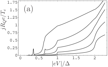
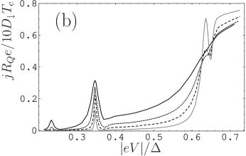
Figure 1: (a) Zero temperature I-V characteristics of dc electric current for $\Theta=0$. $D_{\downarrow}=0.1$, $D_{\uparrow}=0.1$, $0.25$, $0.5$, $0.75$, $1$ from bottom curve to top one. (b) Low-voltage part of I-V characteristics for $\Theta=0$ and $D_{\uparrow}=1$. $D_{\downarrow}=0.02$ (gray solid line), $0.05$ (dashed line), $0.1$ (dotted line) and $0.2$ (solid line). The current $j$ is measured in units $jR_{Q}e/T_{c}$ for the panel (a) and in units $jR_{Q}e/10D_{\downarrow}T_{c}$ for the panel (b). The voltage $|eV|$ is measured in units of superconducting order parameter $\Delta$.

We are interested in the case $eV\sim\Delta$ and high enough transparencies of the junction for one spin direction. Under these conditions Keldysh Green’s function can not be interpreted as a product of density of states and nonequilibrium distribution function. There is an external frequency $2eV$ in the problem under consideration and the above interpretation is only possible in the limit $eV\ll\Delta$. Nevertheless the subharmonic gap structure results from MAR processes between energies corresponding to the poles and continuum spectrum edges of the Green’s function. Therefore we analyze the characteristic features of the Green’s function. For the case $D_{\downarrow}\to 0$ it can be done analytically. The time-independent component of electron spin-up Green’s function $\check{g}_{0,\uparrow}(\epsilon)$ at $D_{\downarrow}\to 0$ and $D_{\uparrow}=1$ has the poles at energies (see Eq.(30) of Appendix)

$$\varepsilon_{1\uparrow}(V)={\rm sgn}\left[\cos\Theta\right]\sqrt{\frac{(\Delta^{2}\cos^{2}\Theta)/2-\left(eV/2\right)^{2}(1-\sin\Theta)}{1+\sin\Theta}}+\frac{eV}{2},~{}~{}~{}|eV|<\Delta(1+\sin\Theta)$$ (11)

$$\varepsilon_{2\uparrow}(V)=-{\rm sgn}\left[\cos\Theta\right]\sqrt{\frac{(\Delta^{2}\cos^{2}\Theta)/2-\left(eV/2\right)^{2}(1+\sin\Theta)}{1-\sin\Theta}}+\frac{eV}{2},~{}~{}~{}|eV|<\Delta(1-\sin\Theta)$$ (12)

These expressions are given for an arbitrary value of spin mixing parameter $\Theta$. The poles (11), (12) of spin-up Green’s function are identical for left and right sides of the interface. The poles of $\check{g}_{0,\downarrow}(\epsilon)$ are obtained from Eqs.(11), (12) by the substitution $\Theta\to-\Theta$ and adding the term $eV{\rm sgn}x$ to the expressions (11) and (12). The corresponding hole Green’s functions at $x<0$ have the poles at the opposite energies $-\varepsilon_{1,2\uparrow}$ and $-\varepsilon_{1,2\downarrow}$.

With decreasing of $D_{\uparrow}$ the poles (11), (12) continuously evolve to the position of Andreev bound states at impenetrable magnetic surface $\varepsilon_{\uparrow}={\rm sgn}\left[\sin(\Theta/2)\right]\cos(\Theta/2)+eV(1+{\rm sgn}x)/2$Fogelstrom00 and merge with the edge of continuum spectrum in the absence of spin mixing $\Theta=0$. The analytical expressions for the poles of Green’s function at $D_{\uparrow}<1$ are quite cumbersome, and so we do not write them here.

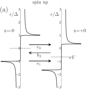
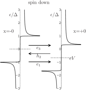
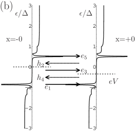
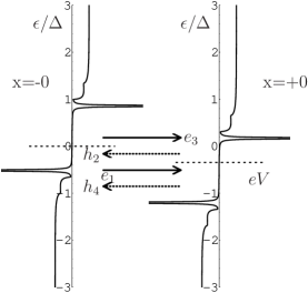
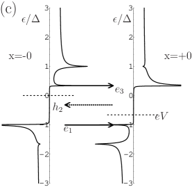
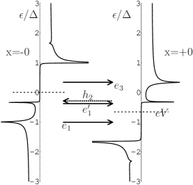
Figure 2: Keldysh part of electron Green’s function as a function of energy. Energy is measured in units of $\Delta$. Each figure represents Green’s functions for left ($x=-0$) and right ($x=+0$) sides of the interface. Left column correspond to spin-up Green’s function and right column to spin-down one. The tunnel limit is presented in panel (a). Panel (b) illustrates the large spin filtering case $D_{\uparrow}=1$, $D_{\downarrow}\to 0$ and panel (c) corresponds to the intermediate case $D_{\uparrow}=0.5$, $D_{\downarrow}\to 0$. Spin mixing angle $\Theta=0$. Horizontal arrows show quasiparticles, which take part in MAR processes. Solid arrows describe electrons and dashed ones correspond to holes. Hole Green’s function is not presented in the figures, but it can be easily obtained from the electron one (see text). The particular voltages taken for the figures are: $|eV|=0.67$ for panel (a), $|eV|=0.34\Delta$ for panel (b) and $|eV|=0.67\Delta$ for panel (c).

To define the subharmonic gap features positions we make use of semiconductor representation. Keldysh part of electron Green’s function $g^{K}_{0,\uparrow,\downarrow}/(-2\pi i)$ for $D_{\downarrow}\to 0$ is presented in Fig.2 as a function of energy for left and right side of the constriction. The temperature is assumed to have zero value. Let $\epsilon=0$ correspond to the Fermi level of the left superconductor, that is $\varepsilon_{F1}=0$. Then for the right superconductor $\varepsilon_{F2}=eV$. We begin by the considering of the tunnel case $D_{\uparrow,\downarrow}\to 0$. This limit is well-known and we only discuss it for comparison to the large spin filtering limit. The corresponding situation is depicted in the panel (a). There are no difference between spin-up and spin-down quasiparticles for $\Theta=0$ and $D_{\uparrow,\downarrow}\to 0$ and so spin-up and spin-down Green’s functions coincide in this case. The only characteristic feature of Green’s function is a square-root singularity at the edge of continuum spectrum. Green’s functions for left and right side of the junction are denoted by the upper case symbols $l,r$. In the tunnel limit $g^{r}(\epsilon)=g^{l}(\epsilon-eV)$ as it is seen in Fig.2(a). Let an electron $e_{1}$ with energy $\epsilon=-\Delta$ pass through the junction region to the right. For $|eV|<2\Delta$ it undergoes Andreev reflection in the right lead and a hole $h_{2}$ with energy $\epsilon=\Delta+2eV$ travels to the left. Then the whole process repeats until an electron in the right lead or a hole in the left lead meets continuum spectrum edge. For an electron $e_{2k+1}$ the condition is $-\Delta-2eVk=\Delta+eV$ and for a hole $h_{2k}$ $2eVk+\Delta=-\Delta$. Consequently, the subharmonic gap steps take place at $|eV|=2\Delta/n$, as it should be.

Fig.2(b) represents the large spin-filtering case $D_{\downarrow}\to 0$, $D_{\uparrow}=1$. For $eV<\Delta$ the most pronounced characteristic features of Green’s function are pole-like singularities. The energies of the poles are given by the expressions (11) and (12). For $eV>\Delta$ the poles merge with the continuum spectrum edge and transform to the gap edge singularities, which disappear when voltage increases further. The subharmonic gap peaks in this case result from MAR processes between the poles of Green’s function. It is important that the poles of spin-up Green’s function are located at the same energies for both sides of the interface. A spin-up electron $e_{1\uparrow}$ with the energy $\varepsilon_{1\uparrow}$ passing through the junction region to the right converts to Andreev reflected hole with the energy $-\varepsilon_{1\uparrow}+2eV$, which travels to the left. Then the process repeats until an electron $e_{2k+1}$ having the energy $\varepsilon_{1\uparrow}-2eVk$ meets the other pole at $\varepsilon_{2\uparrow}$, or a hole with the energy $-\varepsilon_{1\uparrow}+2eVk$ meets the pole of the hole Green’s function at $-\varepsilon_{2\uparrow}$. As a result subharmonic gap peaks appear at

$$|eV_{k}|=(\varepsilon_{2\uparrow}-\varepsilon_{1\uparrow})/2k\enspace.$$ (13)

For the absence of spin mixing this equation gives the following positions of subgap peaks

$$V_{k}=\frac{\Delta}{\sqrt{2k^{2}+1/2}}\enspace.$$ (14)

For low enough voltages (in fact, for $n>2$) we come to the approximate formula by A.Martin-Rodero $\it et.al.$ $eV_{k}=\Delta/\sqrt{2}k$ Cuevas01 . Analogously, as it is seen from Fig.2(b), for spin-down electron MAR processes repeat until an electron $e_{2k+1}$ having the energy $\varepsilon_{1\downarrow}-2eVk$ meets the other pole at $\varepsilon_{2\downarrow}+2eV$, or a hole with the energy $-\varepsilon_{1\downarrow}+2eVk$ meets the pole of the hole Green’s function at $-\varepsilon_{2\downarrow}$. It is worth to note that for spin-down Green’s function the pole energies in the right superconductor are shifted to $\varepsilon_{1,2\downarrow}+2eV$ in comparison to the pole energies $\varepsilon_{1,2\downarrow}$ in the left one. Taking into account the fact that in the left superconductor $\varepsilon_{1,2\downarrow}=-\varepsilon_{2,1\uparrow}$ one obtains the same peak locations as for spin-up current. However, for spin-up current the peak at $eV_{k}$ arises from $2k^{\rm th}$ and $(2k+1)^{\rm th}$ order MAR processes, while for spin-down current the peak at the same voltage results from $(2k-1)^{\rm th}$ and $2k^{\rm th}$ order MAR processes.

For $eV>\Delta$ the poles of Green’s function merge with the gap edge and even gap edge singularities disappear upon further increase of the voltage. For this reason at $eV>\Delta$ MAR processes between gap edges manifest itself in I-V characteristic only by the changes of the slope.

And, finally, intermediate case $D_{\downarrow}\to 0$, $D_{\uparrow}=0.5$ is presented in Fig.2(c). In the intermediate regime Green’s function manifests two types of singularities: the pole-like singularities coming from the large spin filtering case and the gap edge singularities, which are characteristic for the tunneling limit. When $D_{\uparrow}$ gets smaller the upper singularity of $g^{r}_{\uparrow}$ tends to $\Delta+eV$ and the pole at $\varepsilon_{1\uparrow}$ disappears. And, vice versa, for $g^{l}_{\uparrow}$ the pole at $\varepsilon_{2\uparrow}$ disappears, while the bottom singularity tends to $-\Delta$. Correspondingly, spin-up current continuously evolves between the two limits. For spin-down current there is an analogous picture.

The subgap structure smears out with increasing of $D_{\downarrow}$ due to the fact that for non-zero values of $D_{\downarrow}$ Green’s function poles transform to the broadened peaks. It is illustrated in Fig.1(b), where the subharmonic gap structure in the limit $D_{\uparrow}=1$ is presented for several values of spin-down transparency from $D_{\downarrow}=0.02$ up to $D_{\downarrow}=0.2$.

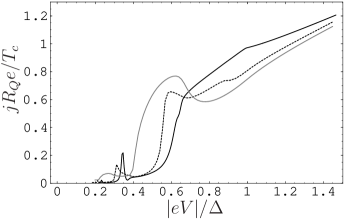
Figure 3: Zero temperature I-V characteristics of dc electric current for $D_{\uparrow}=1$, $D_{\uparrow}=0.1$. $\Theta=0$ (solid line), $\Theta=0.25\pi$ (dotted line), $\Theta=\pi/2$ (gray solid line).

Now let us turn to the effect of spin mixing on the subgap features discussed above. This is illustrated in Fig.3 for $D_{\uparrow}=1$, $D_{\downarrow}=0.1$ and $\Theta=0$, $0.25\pi$ and $\pi/2$. As it can be seen from Eqs.(11),(12), the voltage range where one of the poles exists shrinks with increasing $\Theta$, while it enlarges for the other pole. As a result the peak structure, describing by Eq.(13) only exists at lower voltage range when $\Theta$ grows. For $|eV|>\Delta(1-\sin\Theta)$ one of the poles merges with the edge of the continuum spectrum and evolves to the gap edge singularity. For this reason the peaks get wider with increasing spin mixing. At the same time the peak onsets are practically not shifted due to weak dependence of the pole energies on $\Theta$. It is seen in Fig.3 for $\Theta=0.25\pi$. With further increasing of spin mixing parameter $\Theta$ the gap edge singularity becomes less pronounced and finally disappears. This results in evolving of the peak structure to the hump structure with sharp onsets, as it is illustrated in Fig.3 for $\Theta=\pi/2$. Nevertheless, the hump onsets are well described by the equation (13).

IV Conclusion

The influence of spin filtering and spin mixing, which characterize magnetic interface, on the I-V characteristics of dc electric current for magnetic quantum point contact with superconducting leads is investigated. It is found that with increasing of spin filtering the subharmonic step structure of the dc electric current, typical for low-transparency junction and a junction without spin filtering qualitatively changes. In the lower voltage region the peak structure arises and for higher voltages the slope of I-V characteristic only changes. The subharmonic features are explained in terms of MAR processes between Green’s function singularities and their positions are obtained analytically. In particular, it is found that for large spin filtering the subgap feature at $eV_{k}$ arises from $2k^{\rm th}$ and $(2k+1)^{\rm th}$ order MAR processes for spin-up current and $(2k-1)^{\rm th}$ and $2k^{\rm th}$ order MAR processes for spin-down current. This is in sharp contrast with the tunnel limit, where the step at $eV_{n}$ is known to result from $n^{\rm th}$ order MAR process. The spin mixing results in shrinking of the voltage range where peak structure exists and evolving of the peak structure to the hump structure with sharp onsets.

V Acknowledgments

The support by RFBR Grants 05-02-17175 (I.V.B. and A.M.B.), 05-02-17731 (A.M.B.) and the programs of Physical Science Division of RAS is acknowledged. I.V.B. was also supported by the Russian Science Support Foundation and RF Presidential Grant No.MK-4605.2007.2

*

Appendix A

Substituting the Riccati coherence and distribution functions Eqs. (6), (7) and $(\hat{\Gamma}_{1,2}^{R,A},\hat{\tilde{\Gamma}}_{1,2}^{R,A},\hat{X}_{1,2}^{K},\hat{\tilde{X}}_{1,2}^{K})$ into Eq.(2), after some straightforward algebra we obtain full Green’s function. The Keldysh part of the Green’s function at $x=-0$ corresponding to the incoming trajectory has the following form

$$\frac{\hat{g}^{K}({\bm{p}}_{f})}{-2i\pi}=\hat{\kappa}_{1}\otimes\hat{x}_{1}^{K}\otimes\hat{\kappa}_{1}^{*}-\hat{\kappa}_{2}\otimes{\hat{\tilde{x}}}_{1}^{K}\otimes\hat{\kappa}_{2}^{*}+$$

$$\hat{\kappa}_{3}\otimes\hat{x}_{2}^{K}\otimes\hat{\kappa}_{3}^{*}-\hat{\kappa}_{4}\otimes{\hat{\tilde{x}}_{2}}^{K}\otimes\hat{\kappa}_{4}^{*}\enspace.$$ (15)

Here $~{}^{*}$ means complex conjugation. $\hat{\kappa}_{1,2,3,4}$ are diagonal matrices in spin space and depend on quasiparticle energy $\epsilon$ and time $t$. They can be explicitly written in terms of $S$-matrix elements (9), (10) as follows

$$\kappa_{1\uparrow,\downarrow}=\gamma(\epsilon)\otimes A^{-1}_{\uparrow,\downarrow}(\epsilon,t)\otimes\frac{e^{\displaystyle\mp i\Theta}-\gamma^{2}(\epsilon+eV)\sqrt{R_{\uparrow}R_{\downarrow}}+\gamma(\epsilon)\gamma(\epsilon+eV)\alpha\sqrt{D_{\uparrow}D_{\downarrow}}e^{\displaystyle-2ieVt}}{\sqrt{R_{\downarrow,\uparrow}}e^{\displaystyle\mp i\Theta/2}-\gamma^{2}(\epsilon+eV)\sqrt{R_{\uparrow,\downarrow}}e^{\displaystyle\pm i\Theta/2}}\otimes\frac{1}{\gamma(\epsilon)}\enspace,$$ (16)

$$\kappa_{2\uparrow,\downarrow}=\gamma(\epsilon)\otimes A^{-1}_{\uparrow,\downarrow}(\epsilon,t)\enspace,$$ (17)

$$\kappa_{3\uparrow,\downarrow}=\pm i\kappa_{1\uparrow,\downarrow}\otimes\frac{\sqrt{D_{\uparrow,\downarrow}}e^{\displaystyle\mp i\Theta/2}-\gamma(\epsilon-eV)\gamma(\epsilon)\sqrt{D_{\downarrow,\uparrow}}e^{\displaystyle\pm i\Theta/2}e^{\displaystyle 2ieVt}}{\sqrt{R_{\uparrow,\downarrow}}e^{\displaystyle\mp i\Theta/2}-\gamma^{2}(\epsilon-eV)\sqrt{R_{\downarrow,\uparrow}}e^{\displaystyle\pm i\Theta/2}}\mp$$

$$i\frac{\sqrt{D_{\uparrow,\downarrow}}e^{\displaystyle\mp i\Theta/2}}{\sqrt{R_{\uparrow,\downarrow}}e^{\displaystyle\mp i\Theta/2}-\gamma^{2}(\epsilon-eV)\sqrt{R_{\downarrow,\uparrow}}e^{\displaystyle\pm i\Theta/2}}\enspace,$$ (18)

$$\kappa_{4\uparrow,\downarrow}=\pm i\kappa_{2\uparrow,\downarrow}\otimes\frac{\sqrt{D_{\downarrow,\uparrow}}e^{\displaystyle\mp i\Theta/2}-\gamma(\epsilon+eV)\gamma(\epsilon)\sqrt{D_{\uparrow,\downarrow}}e^{\displaystyle\pm i\Theta/2}e^{\displaystyle-2ieVt}}{\sqrt{R_{\downarrow,\uparrow}}e^{\displaystyle\mp i\Theta/2}-\gamma^{2}(\epsilon+eV)\sqrt{R_{\uparrow,\downarrow}}e^{\displaystyle\pm i\Theta/2}}\enspace,$$ (19)

where we use a notation

$$\gamma(\epsilon)=\left\{\begin{array}[]{l}(\epsilon-i\sqrt{\Delta^{2}-\epsilon^{2}})/\Delta,~{}~{}~{}~{}~{}~{}|\epsilon|<\Delta\\ (\epsilon-{\rm sgn}\epsilon\sqrt{\epsilon^{2}-\Delta^{2}})/\Delta,~{}~{}|\epsilon|>\Delta\enspace.\end{array}\right.$$ (20)

Quasiparticle energy $\epsilon$ has infinitesimal imaginary part $\delta>0$. For numerical integration over $\epsilon$ we introduce finite $\delta=0.003\Delta$, which models inelastic scattering.

Keldysh Green’s function $g(\underline{\bm{p}}_{f})$ for outgoing trajectory can be obtain from Eq.(15) by the following procedure

$$\frac{g_{\uparrow,\downarrow}^{K}(\underline{\bm{p}}_{f})}{-2i\pi}=\frac{1}{\gamma(\epsilon)}\otimes\biggl{\{}\frac{g_{\downarrow,\uparrow}^{K}({\bm{p}}_{f},-V,-\Theta)}{-2i\pi}+$$

$$2{\rm Re}\left[\kappa_{1\downarrow,\uparrow}(-V,-\Theta)\otimes\tilde{x}^{K}_{1}\right]+x^{K}_{1}\biggr{\}}\otimes\frac{1}{(\gamma(\epsilon))^{*}}\enspace.$$ (21)

The function $A^{-1}_{\uparrow,\downarrow}(\epsilon,t)$ is inverse to

$$A_{\uparrow,\downarrow}(\epsilon,t)=a_{0\uparrow,\downarrow}(\epsilon)+a_{1\uparrow,\downarrow}(\epsilon)(e^{-2ieVt}+e^{2ieVt})\enspace,$$ (22)

$$a_{0\uparrow,\downarrow}(\epsilon)=\frac{e^{\displaystyle\mp i\Theta}-\sqrt{R_{\uparrow}R_{\downarrow}}(\gamma^{2}(\epsilon)+\gamma^{2}(\epsilon+eV))+\gamma^{2}(\epsilon)\gamma^{2}(\epsilon+eV)R_{\uparrow,\downarrow}e^{\displaystyle\pm i\Theta}}{\sqrt{R_{\downarrow,\uparrow}}e^{\displaystyle\mp i\Theta/2}-\gamma^{2}(\epsilon+eV)\sqrt{R_{\uparrow,\downarrow}}e^{\displaystyle\pm i\Theta/2}}+$$

$$\frac{D_{\uparrow,\downarrow}e^{\displaystyle\pm i\Theta}\gamma^{2}(\epsilon)\gamma^{2}(\epsilon-eV)}{\sqrt{R_{\downarrow,\uparrow}}e^{\displaystyle\mp i\Theta/2}-\gamma^{2}(\epsilon-eV)\sqrt{R_{\uparrow,\downarrow}}e^{\displaystyle\pm i\Theta/2}}\enspace,$$ (23)

$$a_{1\uparrow,\downarrow}(\epsilon)=\frac{\alpha\sqrt{D_{\uparrow}D_{\downarrow}}\gamma(\epsilon)\gamma(\epsilon+eV)}{\sqrt{R_{\downarrow,\uparrow}}e^{\displaystyle\mp i\Theta}/2-\gamma^{2}(\epsilon+eV)\sqrt{R_{\uparrow,\downarrow}}e^{\displaystyle\pm i\Theta/2}}\enspace.$$ (24)

The function $A^{-1}$ is of great importance for us because it contains all the essential singularities of the Green’s function giving rise to the subgap features in the I-V characteristics. In general, it has the form

$$A^{-1}_{\uparrow,\downarrow}=\sum\limits_{m=-\infty}^{\infty}\rho_{m\uparrow,\downarrow}(\epsilon)e^{2ieVmt}\enspace.$$ (25)

The condition $A^{-1}(\epsilon,t)\otimes A(\epsilon,t)\equiv 1$ leads to the following recurrent equation for $\rho_{m\uparrow,\downarrow}(\epsilon)$

$$\rho_{m\uparrow,\downarrow}(\epsilon)a_{0\uparrow,\downarrow}(\epsilon+eVm)+$$

$$\rho_{m-1\uparrow,\downarrow}(\epsilon-eV)a_{1\uparrow,\downarrow}(\epsilon+eV(m-1))+$$

$$\rho_{m+1\uparrow,\downarrow}(\epsilon+eV)a_{1\uparrow,\downarrow}(\epsilon+eV(m+1))=\delta_{m0}$$ (26)

with the asymptotic conditions $\rho_{m}(\epsilon)\to 0$ for $m\to\pm\infty$. In order to obtain Eq.(26) one should use the following rule

$$c_{1}(\epsilon)e^{2ieVmt}\otimes c_{2}(\epsilon)e^{2ieVnt}=$$

$$c_{1}(\epsilon-eVn)c_{2}(\epsilon+eVm)e^{2ieV(m+n)t}\enspace,$$ (27)

which is valid for any integer $m$ and $n$ and can be easily deduced from the general definition of the noncommutative convolution. For arbitrary values of parameters $D_{\uparrow}$ and $D_{\downarrow}$ we find the coefficients $\rho_{m\uparrow,\downarrow}(\epsilon)$ numerically making use of Eq.(26). However, for the case $a_{1}(\epsilon)=0$ $A^{-1}$ can be easily found analytically. Then the function $A$ does not depend on time and

$$A^{-1}_{\uparrow,\downarrow}(\epsilon)=\frac{1}{a_{0\uparrow,\downarrow}}\enspace.$$ (28)

There are two special cases when Eq.(28) is valid. The first one is the impenetrable surface $D_{\uparrow}=D_{\downarrow}=0$. Then the poles of the Green’s functions, which are determined by the equation

$$a_{0\uparrow,\downarrow}(\epsilon)=0\enspace,$$ (29)

correspond to the well-known energies of Andreev bound states at impenetrable magnetic surface $\varepsilon_{\uparrow,\downarrow}=\pm{\rm sgn}\left[\sin(\Theta/2)\right]\cos(\Theta/2)$ Fogelstrom00 .

The second limit corresponds to full spin-filtering $D_{\downarrow}=0$ (or $D_{\uparrow}=0$) and arbitrary transparency of the other spin channel. In this case the Green’s function also has the poles. The energies of the poles at $x<0$ can be obtained from Eq.(29), which for spin-up quasiparticles is reduced to (we assume $D_{\downarrow}$ to be zero)

$$e^{-i\Theta}-(\gamma^{2}(\epsilon-eV)+\gamma^{2}(\epsilon))\sqrt{R_{\uparrow}}+$$

$$\gamma^{2}(\epsilon-eV)\gamma^{2}(\epsilon)e^{i\Theta}=0\enspace.$$ (30)

The pole equation for spin-down quasiparticles is obtained from (30) by the substitution $\Theta\to-\Theta$ and $\epsilon\to\epsilon+eV$. The poles of spin-up Green’s function at $x>0$ are the same as at $x<0$. For spin-down quasiparticles they are to be deduced from Eq.(30) substituting $\epsilon-eV$ for $\epsilon$ and changing sign of $\Theta$. The explicit expressions of the pole energies are quite cumbersome for arbitrary $D_{\uparrow}$. They are only written for the special case $D_{\uparrow}=1$ (see Eqs.(11) and (12)). It is worth to note that in the case $D_{\uparrow}D_{\downarrow}\neq 0$ the function $A$ depends on time and, consequently, $A^{-1}$ has no true poles. That is the reason for smearing of subgap features when $D_{\downarrow}$ increases.

References

- (1) T.M. Klapwijk, G.E. Blonder, and M. Tinkham, Physica B+C 109-110, 1657 (1982).
- (2) M. Octavio, M. Tinkham, G.E. Blonder, and T.M. Klapwijk, Phys.Rev.B 27, 6739 (1983); K. Flensberg, J.Bindslev Hansen, and M. Octavio, ibid. 38, 8707 (1988).
- (3) G.B. Arnold, J.Low Temp.Phys. 68, 1 (1987).
- (4) E.N. Bratus’, V.S. Shumeiko, and G.Wendin, Phys. Rev. Lett. 74, 2110 (1995).
- (5) D. Averin and A. Bardas, Phys. Rev. Lett. 75, 1831 (1995).
- (6) J.C. Cuevas, A. Martin-Rodero, and A. Levy-Yeyati, Phys. Rev. B 54, 7366 (1996).
- (7) A. Ingerman, G. Johansson, V.S. Shumeiko, and G. Wendin, Phys. Rev. B, 64, 144504 (2001); P. Samuelsson, A. Ingerman, G. Johansson, E.V. Bezuglyi, V.S. Shumeiko, and G. Wendin, ibid. 70, 212505 (2004).
- (8) A. Bardas, and D.V. Averin, Phys.Rev. B, 56, 8518 (1997).
- (9) A.V. Zaitsev, and D.V. Averin, Phys. Rev. Lett. 80, 3602 (1998).
- (10) P. Samuelsson, G. Johansson, A. Ingerman, V.S. Shumeiko, and G. Wendin, Phys. Rev. B, 65, 180514, (2002).
- (11) E.V. Bezuglyi, E.N. Bratus’, V.S. Shumeiko, and G. Wendin, Phys. Rev. Lett. 83, 2050 (1999).
- (12) E.V. Bezuglyi, E.N. Bratus’, V.S. Shumeiko, G. Wendin, and H.Takayanagi, Phys. Rev. B, 62, 14439, (2000).
- (13) A. Brinkman, A.A. Golubov, H. Rogalla, F.K. Wilhelm, and M.Yu. Kupriyanov, Phys. Rev. B 68, 224513 (2003).
- (14) J.C. Cuevas, J. Hammer, J. Kopu, J.K. Viljas, and M. Eschrig, Phys.Rev.B 73, 184505 (2006).
- (15) N. van der Post, E.T. Peters, I.K. Yanson, and J.M. van Ruitenbeek, Phys. Rev. Lett. 73, 2611 (1994).
- (16) E.Scheer, P.Joyez, D.Esteve, C.Urbina, and M.H. Devoret, Phys. Rev. Lett. 78, 3535 (1997).
- (17) E. Scheer, N.Agrait, J.C. Cuevas, A. Levy-Yeyati, B. Ludoph, A. Martin-Rodero, G.R. Bollinger, J.M. van Ruitenbeek, and G. Urbina, Nature (London) 394, 154 (1998).
- (18) B. Ludoph, N. van der Post, E.N. Bratus’, E.V. Bezuglyi, V.S. Shumeiko, G. Wendin, and J.M. van Ruitenbeek, Phys. Rev. B, 61, 8561 (2000).
- (19) J. Kutchinsky et al., Phys.Rev.B 56, R2932 (1997); R. Taboryski et al., Superlattices Microstruct. 25, 829 (1999).
- (20) T. Hoss, C. Strunk, T. Nussbaumer, R. Huber, U. Staufer, and C. Schönenberger, Phys.Rev.B 62, 4079 (2000).
- (21) A. Martin-Rodero, A. Levy Yeyati, J.C. Cuevas Physica C, 352, 117 (2001).
- (22) M. Andersson, J.C. Cuevas, M.Fogelström, Physica C, 367, 117 (2002).
- (23) I.V. Bobkova, Phys.Rev.B 73, 012506 (2006).
- (24) I.V. Bobkova and A.M. Bobkov, unpublished notes.
- (25) Erhai Zhao and J.A. Sauls, Phys. Rev. Lett. 98 , 206601 (2007).
- (26) M. Eschrig, Phys. Rev. B 61, 9061 (2000).
- (27) M. Fogelström, Phys. Rev. B, 62, 11812 (2000).
- (28) Erhai Zhao, Tomas Lofwander, and J.A. Sauls Phys. Rev. B 70, 134510 (2004).
- (29) Yu. S. Barash and I. V. Bobkova, Phys. Rev. B 65, 144502 (2002).