On the evolution of eccentric and inclined protoplanets embedded in protoplanetary disks

Abstract

Context. Young planets embedded in their protoplanetary disk interact gravitationally with it leading to energy and angular momentum exchange. This interaction determines the evolution of the planet through changes to the orbital parameters.

Aims. We investigate changes in the orbital elements of a 20 Earth–mass planet due to the torques from the disk. We focus on the non-linear evolution of initially non-vanishing eccentricity, $e$, and/or inclination, $i$.

Methods. We treat the disk as a two- or three-dimensional viscous fluid and perform hydrodynamical simulations using finite difference methods. The planetary orbit is updated according to the gravitational torque exerted by the disk. We monitor the time evolution of the orbital elements of the planet.

Results. We find rapid exponential decay of the planet orbital eccentricity and inclination for small initial values of $e$ and $i$, in agreement with linear theory. For larger values of $e>0.1$ the decay time increases and the decay rate scales as $\dot{e}\propto e^{-2}$, consistent with existing theoretical models. For large inclinations ($i>6^{\circ}$) the inclination decay rate shows an identical scaling $di/dt\propto i^{-2}$. We find an interesting dependence of the migration on the eccentricity. In a disk with aspect ratio $H/r=0.05$ the migration rate is enhanced for small non-zero eccentricities ($e<0.1$), while for larger values we see a significant reduction by a factor of $\sim 4$. We find no indication for a reversal of the migration for large $e$, although the torque experienced by the planet becomes positive when $e\simeq 0.3$. This inward migration is caused by the persisting energy loss of the planet.

Conclusions. For non gap forming planets, eccentricity and inclination damping occurs on a time scale that is very much shorter than the migration time scale. The results of non linear hydrodynamic simulations are in very good agreement with linear theory for values of $e$ and $i$ for which the theory is applicable (i.e. $e$ and $i\leq H/r$).

1 Introduction

In the early stages of their formation protoplanets are still embedded in the disk from which they formed. Not only will the protoplanet accrete material from the disk, it will also interact gravitationally with it. Planet-disk interaction is an important aspect in the process of planet formation, and has been studied already before the discovery of extrasolar planets through linear analysis (Goldreich & Tremaine 1980; Papaloizou & Lin 1984; Ward 1986). In more recent times this was followed up by non-linear numerical simulations using a two-dimensional setup (Bryden et al. 1999; Kley 1999; Lubow et al. 1999; D’Angelo et al. 2002) and later in three dimensions as well (D’Angelo et al. 2003; Bate et al. 2003; Schäfer et al. 2004).

Since detection of the first extrasolar planet in 1995 there have been about 200 additional discoveries (for an up-to-date list see e.g. http://exoplanet.eu/ by J.Schneider). One of the surprising differences between our own Solar System and these extrasolar planets are their orbital properties. In the Solar System the larger (giant) planets move on almost circular orbits, whereas in contrast most extrasolar planets move on eccentric orbits. For a recent overview see Marcy et al. (2005). The average orbital eccentricity of observed extrasolar planets is $e\simeq 0.3$. Not only are massive planets of several Jupiter masses found in eccentric orbits, but so are lighter planets in the mass range where they cannot open a clean gap in the disk ($M<M_{Jup}$).

One possible origin of the eccentricity is through interaction with the protoplanetary disk. In particular, Goldreich & Sari (2003), Sari & Goldreich (2004) estimate that eccentric Lindblad resonances can cause eccentricity growth for gap forming planets. On the other hand, linear studies, for example by Ward (1988), Papaloizou & Larwood (2000) and Tanaka & Ward (2004), predict eccentricity damping for low mass embedded planets. Numerical hydrodynamical simulations of embedded planets tend to show eccentricity damping as well. For example Papaloizou et al. (2001) find eccentricity growth for bodies on initially circular orbits, but only for companions with a mass greater than 10 $M_{Jup}$. A recent study by D’Angelo et al. (2006), however, suggests that modest disk induced eccentricity growth can occur for planet masses in the Jovian mass range. The origin of the on-average higher eccentricities of the extrasolar planets remains to be definitively addressed, although recent work indicates good agreement between planetary scattering simulations and observational data (Juric & Tremaine 2007).

The linear estimates of the eccentricity evolution of embedded planets (Artymowicz 1993; Ward & Hahn 1994; Tanaka & Ward 2004) concentrate on small eccentricities and predict exponential decay on short timescales $\tau_{ecc}\approx(H/r)^{2}\tau_{mig}$, where $H/r$ is the aspect ratio of the disk and $\tau_{mig}$ and $\tau_{ecc}$ the migration and eccentricity damping time scale, respectively. Papaloizou & Larwood (2000) have also considered larger values for $e$ and they find an extended eccentricity damping time scale such that $de/dt\propto e^{-2}$ if $e>1.1H/r$. Additionally they find positive torques acting on the planet for large values of $e$ and interpret this as outward migration. Recently, Cresswell & Nelson (2006) have performed hydrodynamical simulations of embedded small mass planets and find good agreement with the work by Papaloizou & Larwood (2000).

The influence of the disk on the inclination of the planet has only been analysed in linear studies by Tanaka & Ward (2004). They find exponential damping for any non-vanishing inclinations on similar timescales as the eccentricity damping. In both cases, their results are formally valid only for $e,i\ll H/r$, but numerical experiments (Cresswell & Nelson 2006) suggest that at least their eccentricity damping estimates may be valid for a larger range of values and for a variety of sub-gap opening planet masses.

Here we investigate the dynamical influence the protoplanetary disk has on a protoplanet on an eccentric and/or inclined orbit. To model the disk dynamics we use a fully non-linear hydrodynamical description in both two and three dimensions. The orbit of the embedded planet is allowed to evolve due to the torques from the disk. While in Kley & Dirksen (2006) the possibility of eccentricity growth within the disk due to high mass planets ($>$ 1 Jupiter mass) has been studied, we now analyse the planet-disk interaction of a low-mass planet of 20 Earth masses. Our work extends the recent two-dimensional analysis of Cresswell & Nelson (2006). We vary the initial orbit parameters and analyse the influence of a nonzero eccentricity and inclination on the migration rate of the planet. In particular we investigate if there are important differences between the circular, the low eccentricity and the high eccentricity regimes. We analyse the time scale of the eccentricity and inclination damping and compare to previous linear analysis. We also compare the migration rates for the different orbital parameters with the circular coplanar case and the analytical values from Tanaka et al. (2002), and determine an experimental upper bound on the validity of the exponential decay of eccentricity and inclination modelled by the analytical estimates of Tanaka & Ward (2004).

This paper is organised as follows. In section 2 we discuss the disk models and numerical methods. In section 3 we discuss the results for planets on initially eccentric orbits located in the disk midplane. In section4 we discuss the results for planets on inclined and/or eccentric orbits. Finally we discuss our results and draw conclusions in section 5

2 The Hydrodynamical Model

To study the evolution of an embedded planet in a protoplanetary disk we treat the disk as a viscous fluid. We consider both 2- and 3-dimensional (2D, 3D) models which enables us to analyse the influence of dimensionality directly. Finding the right setup for the 2D models to agree with the more complex 3D results will enable us to reduce computational efforts in the future. The origin of the coordinate system typically is star centred (in particular for the 2D simulations and those 3D models presented in section 4), but for some simulations it is located at the centre of mass of the planet and star system. The $z=0$ plane defines the disk midplane and the planetary inclination is measured with respect to this plane. Many simulations were performed in a reference system that would be initially corotating with the planet if it were on a circular orbit. This rotation rate is kept constant during the simulations so that we do not have to consider extra accelerations. Simulations presented in section 4 were performed in the inertial frame.

For the 2D models we use cylindrical coordinates ($r,\varphi,z$) and consider a vertically averaged, infinitesimally thin disk located at $z=0$. The basic hydrodynamic equations (mass and momentum conservation) describing the time evolution of such a two-dimensional ($r,\varphi$) disk with embedded planets have been stated frequently and are not repeated here (see Kley 1999). The 2D models presented here are calculated basically in the same manner as those described previously in Kley (1998, 1999) using the code RH2D. The reader is referred to those papers for details on the computational aspects of this type of simulations. Other similar models, following explicitly the motion of single planets in disks, have been presented by Nelson et al. (2000) and Bryden et al. (2000).

For the 3-dimensional models we work in spherical coordinates ($r,\varphi,\theta$) where in the third dimension we use a Gaussian density profile, consistent with a locally isothermal equation of state. We also set $H/r=const.$ In the vertical direction the grid extends over several scale heights. This approach is the same as that described in Kley et al. (2001) and D’Angelo et al. (2003).

2.1 Initial Setup

The 3D ($r,\varphi,\theta$) computational domain consists of a complete ring of the protoplanetary disk centred on the star. The radial extent of the computational domain (ranging from $r_{\mathrm{min}}$ to $r_{\mathrm{max}}$) is chosen such that there is sufficient space on both sides of the planet to reduce possible influence of the boundaries. Typically, we assume $r_{\mathrm{min}}=0.4$ and $r_{\mathrm{max}}=2.5$ in units where the planet is located initially at $r=1$. In the azimuthal direction for a complete annulus we have $\varphi_{\mathrm{min}}=0$ to $\varphi_{\mathrm{max}}=2\pi$. In the meridional direction we take a wedge spanning several disk scale heights: $\theta_{min}=75^{\circ}$ and $\theta_{max}=105^{\circ}$. To save computer time, the models without inclination were run in half a disk with $\theta_{max}=90^{\circ}$, using symmetry around the midplane. Finally in the 2D simulations we use the same radial extent as in the 3D case.

The initial structure of the disk (density, temperature, and velocity) is axisymmetric. For the density $\rho(r,\varphi,\theta$) we assume a Gaussian stratification in the vertical direction with a scale length $H$, and a power law for the radial dependence

$$\rho(r,\varphi,\theta)=\rho_{0}(r)\,\exp{[-1/2(r\theta/H)^{2}]}$$ (1)

where we choose $\rho_{0}(r)\propto r^{-1.5}$ such that the initial surface density $\sigma(r)=\int\rho dz$ falls off radially as a power law with index -0.5. If there is no planet, this equilibrium density structure will be preserved for constant kinematic viscosity and closed radial boundaries (Kley et al. 2001). The initial velocity is pure Keplerian rotation ($u_{r}=0,u_{\varphi}=(GM_{*}/r)^{1/2},u_{\theta}=0$). The temperature stratification is always given by $T(r)\propto r^{-1}$ which follows from an assumed constant vertical height $H/r=const$. For these locally isothermal models the temperature profile remains fixed and no energy equation is required. We use a constant kinematic viscosity coefficient $\nu$.

To preserve a constant mass in the disk we use reflecting boundary conditions at the inner and outer boundary. For testing purposes we apply also damping boundary conditions as described in de Val-Borro et al. (2006). In the azimuthal direction, periodic boundary conditions for all variables are imposed. At the upper and lower meridional boundary we also use reflecting boundary conditions to preserve the total mass. In those models where only the upper part of the disk is considered we use symmetric boundary conditions at the midplane to simulate a lower half of the disk that is symmetric to the upper half.

2.2 Model parameters

The computational domain is covered by 131 $\times$ 388 $\times$ 40 ($N_{r}\times N_{\varphi}\times N_{\theta}$) grid cells which are spaced equidistant in radius, azimuth and polar angle. Half the number of cells are used in the meridional direction when symmetry about the midplane is assumed.

The mass of the planet relative to the mass of the star in the different models is 6$\times 10^{-5}$, which corresponds to a 20 $M_{\oplus}$ planet for a Solar mass star. We allowed the planetary orbit to evolve as a result of the torque exerted by the disk. In these models we assume a disk mass inside the computational domain ($r=$ 2.08 to 13 AU for a Solar type star) of $7.0\times 10^{-3}M_{\odot}$.

A constant dimensionless kinematic viscosity $\nu=10^{-5}$ is used for all models. This corresponds to $\alpha=0.004$ for a planet at $a=5.2$ AU, a typical value for a protoplanetary disk. We set $H/r=0.05$.

We let the planet evolve to observe the orbital evolution of the system. The motion of the planet is integrated using a fourth order Runge-Kutta integrator where the time step size is given by the hydrodynamical time step. As a test we have run pure 2 and 3-body problems of one star with one or two planets under the same conditions as in the full hydrodynamical evolution (i.e. identical timestep size) and find that the relative total energy loss is less than $6\times 10^{-6}$ for $\approx 2,500,000$ time steps, which is equivalent to several thousand periods of the planet. The forces from the disk material are calculated in first order and are added when the planet positions are updated. Disk self-gravity is not included.

In these models we did not take into account torques (forces) from disk material that lies closer to the planet than $r_{torq}=0.8-1.0\,R_{Hill}$ where the Hill-radius is given by

$$R_{\mathrm{Hill}}=a_{\mathrm{p}}\,\left(\frac{q}{3}\right)^{1/3}$$ (2)

where $a_{p}$ is the actual semi-major axis of the planet orbit. For the calculations in section 3.4 we use a smoothed transition for the torque cutoff.

2.3 Numerical issues

We use two different codes, NIRVANA and RH2D for our calculations. The numerical method used for both utilises a staggered mesh, spatially second order finite difference method based, where advection is based on the monotonic transport algorithm (van Leer 1977). Due to operator-splitting the code is semi-second order in time. Details of the NIRVANA code have been described in Ziegler (1998), where both the London and Tübingen groups have added their own improvements to the code. Application of the two dimensional code RH2D to the embedded planet problem is described in Kley (1998).

The use of a rotating coordinate system in most of our runs requires special treatment of the Coriolis terms to ensure angular momentum conservation (Kley 1998).

In calculating the gravitational potential of the planet we use a smoothed potential of the form

$$\Phi_{P}=-\frac{Gm_{p}}{(s^{2}+\epsilon^{2})^{1/2}}$$ (3)

where $s$ is the distance from the planet. For the smoothing length $\epsilon$ of the potential we choose the diagonal length of one grid cell in three dimensions (this corresponds to 80 % of the Hill sphere radius), and to simulate the three-dimensional environment as well as possible in two dimensions we use $\epsilon=0.6H$.

The viscous terms, including all necessary tensor components, are treated explicitly.

An important issue in complex numerical hydrodynamical simulations is the study of numerical convergence and consistency. While consistency of our difference equations is satisfied through derivation of them from Taylor-expansions, the question of convergence is typically addressed through resolution studies. As described below, the main results of our simulations are obtained by running two- and three-dimensional disk-planet simulations over several hundreds of orbital periods. Since it is not possible to perform resolution studies on all physical setups we present in the next sections the results obtained with our standard resolution ($131\times 388\times 40$ for a 3D-setup with inclined planet). Additional resolution studies performed on a representative sample are described in more detail in the Appendix, and briefly at the relevant description of the results in the text.

3 Eccentricity evolution

For the study of eccentricity damping of a planet embedded in a protoplanetary disk we use here non-inclined orbits and distinguish two different regimes. First we will investigate the regime of low non-zero eccentricity and then we will look at high eccentricities similar to those observed in exoplanetary systems. The time variation $e(t)$ of the planetary eccentricity is shown for different initial eccentricities $e_{0}$ in Fig. 1.

3.1 Low initial eccentricity

If we start the planet with a sufficiently low eccentricity ($e_{0}\leq 0.1$) we observe an exponential decay of the orbital eccentricity of the planet.

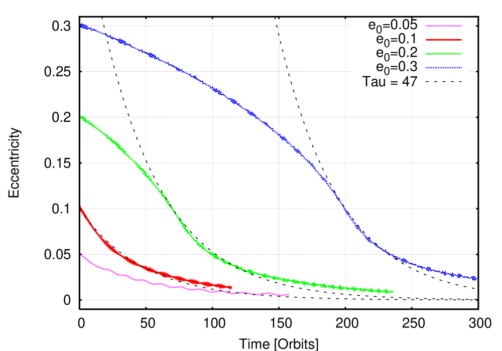
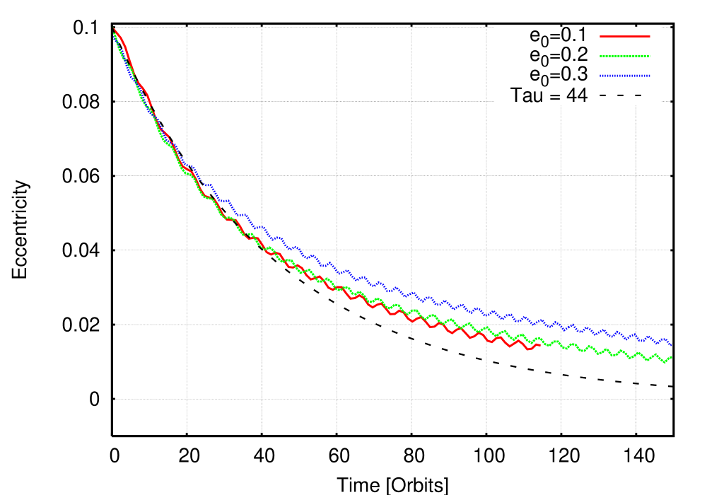
Figure 1: Eccentricity evolution of a 20 $m_{E}$ planet in a 3D protoplanetary disk as a function of time for different initial eccentricities. We find exponential decay in the low-eccentricity regime $e_{0}\leq 0.10$, and slower damping for higher eccentricities. Top: The dashed lines indicate the exponential linear result ($\tau_{ecc}=47$) for this density as derived in Tanaka & Ward (2004). Bottom: Time-shifted results for the late exponential phase of the simulations with large initial $e_{0}\geq 0.1$. The dashed curve indicates here an exponential decay with $\tau_{ecc}=44$.

Figure 2: Semi-major axis evolution of the planet in a 3D protoplanetary disk as a function of time for different initial eccentricities. For small non-zero eccentricities the migration rate increases above the $e=0$ case. For large eccentricities the migration rate is significantly slower.

We find that for the low eccentricity models with $e_{0}\leq 0.10$ the decay time $t_{ecc}=|e/\dot{e}|$ is approximately 44 – 50 orbits. Using linear analysis for small eccentricities Tanaka & Ward (2004) find that the mean eccentricity change (averaged over one planetary orbit) is given by

$$\frac{\overline{de/dt}}{e}=-\frac{0.780}{t_{wave}}$$ (4)

with characteristic time

$$t_{wave}=q^{-1}\left(\frac{\sigma_{p}a^{2}}{M_{*}}\right)^{-1}\left(\frac{c_{s}}{a\Omega_{p}}\right)^{4}\Omega_{p}^{-1}$$ (5)

where $q$ is the mass ratio between the planet and the star, and $\sigma_{p}$ the local surface density at the planetary orbit. For a planet of 20 Earth masses at 5.2 AU in a MMSN nebula ($\sigma_{p}=1490\ {\rm kg\leavevmode\nobreak\ m^{-2}}$), as in our model, the characteristic time is $t_{wave}=438$ yrs $=37$ orbits. This gives an eccentricity damping time scale of about $\tau_{ecc}=t_{wave}/0.78=47$ orbits. This expected exponential eccentricity evolution is indicated in Fig. 1 (upper panel) by the dashed curves for $e_{0}=0.1$ and (shifted) for $e_{0}=0.2$ and $0.3$ matched to the point where the curves cross $e=0.1$. In the lower panel of Fig. 1 we overlay the eccentricity evolution for different $e_{0}$ such that they overlap at $e=0.1$. The exponential decay phase is very similar for the different initial eccentricities (see also below). As seen from the plot our calculated $e$-damping time scale is only differs slightly, being about 44 orbital periods for $e=0.1$ and increasing later as the eccentricity damps further. This increase in damping time relative to that obtained by Tanaka & Ward (2004) is probably due to the influence of the gravitational softening in our 3D simulations.

Overall, the linear estimates of Tanaka & Ward (2004) are therefore in good agreement with our numerical results for eccentricities $e\leq 0.1$. Formally it is expected that agreement should hold for $e\leq H/r$, and for our disks $H/r=0.05$, so the linear estimates appear to be good over twice their formal range of applicability.

As can be seen in Fig. 2 an eccentric orbit will also change the migration rate of the planet. The nearly straight solid line denotes the migration for a planet on a circular orbit with $e_{0}=0.0$. Notice that in this case we always maintain the zero eccentricity. For the eccentric planets the migration rate shows sinusoidal variations that are caused by the orbital variations of the torques acting on the planet.

An interesting effect can be seen when one looks at the migration time scale of the planet. For small initial eccentricities in the exponential damping regime, here $e_{0}=0.05$ and $e_{0}=0.10$, we find a slightly faster migration rate for the planet than in the circular case. This result is obtained for all codes used in this study, and is found in both 2D and 3D runs. Its long term influence on the migration rates of protoplanets is not significant, however, as the eccentricity damping time scale is shorter than the migration time by a factor on the order of $(H/r)^{2}$.

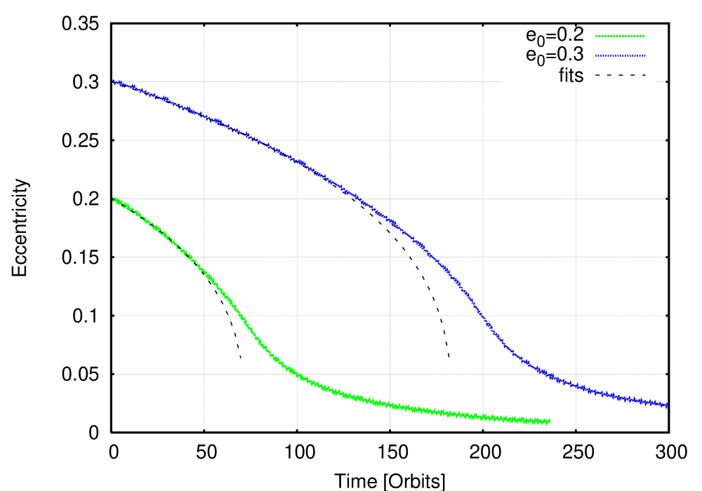
Figure 3: The models with $e_{0}=0.2$ and $0.3$ are fitted to a theoretical model with $\dot{e}\propto{e^{-2}}$. As can be seen this scaling works extremely well as long as the eccentricity is larger than about 2.5 $H/r$.

3.2 High initial eccentricity

If we start the planet with a high eccentricity ($e_{0}>0.1$) we also observe a decay of the orbital eccentricity of the planet, but it is slower and the decay rate is no longer exponential, as can be seen in the two upper curves in Fig. 1. In fact it fits well with the theoretical model described in Papaloizou & Larwood (2000), which predicts $\dot{e}\propto e^{-2}$. In Fig. 3 the calculations with $e_{0}=0.2$ and $0.3$ are fitted with such a model. The fits are extremely good. The characteristic damping time at $t=0$ for this non-exponential damping with $\dot{e}=Ke^{-2}$ is given by

$$\tau_{e}=\left.\frac{e}{\dot{e}}\right|_{t=0}\,=\,\frac{e_{0}^{3}}{K}$$ (6)

From Fig. 3 we obtain $\tau_{e}=71$ for $e_{0}=0.2$, and for $e_{0}=0.3$ we find $\tau_{e}\approx 183$ orbital periods, more than a four-fold increase over the exponential decay. Also notice that when the eccentricity falls beneath the value for which exponential damping occurs, the lines in Fig. 1 (lower panel) look similar to shifted copies of each other, indicating that the planet has no memory of its previously higher eccentricity. In the large $e_{0}=0.3$ case the additional evolution in semi-major axis may account for the observed (slight) difference in decay time.

For these high initial eccentricities we find additionally a reduced migration rate (Fig. 2). In Fig. 4 the relative migration rate compared to the $e=0$ model is plotted. For small eccentricities the migration rate may increase by as much as 60% before dropping off in the manner expected for larger eccentricities. For a large eccentricity of $e=0.3$ the migration rate is 5 times smaller than for a planet on a circular orbit.

Figure 4: The relative initial migration rate as a function of eccentricity for a planet with mass ratio $q=6\times 10^{-5}$. For low eccentricities the migration rate can increase by up to 60%, for high eccentricities we find a substantial slowing of the migration.

Figure 5: The long term evolution of the semi-major axis for different initial eccentricities for a 20 $m_{E}$ planet for 3D models. All models except the one with the largest initial eccentricity converge to the same migration rate, and this large $e$ run eventually converges also after a longer run time.

In the long term evolution of the migration rate we see in Fig. 5 that all models converge to the circular migration rate when approaching $e=0$, as expected. This turnover to the circular migration rate occurs at a residual eccentricity of about $e=0.05\approx H/r$, i.e. for the model with $e_{0}=0.10$ at around $t=20$ and for the model with $e_{0}=0.2$ at around $t=80$. For the $e=0.3$ model the eccentricity has not dropped enough to reach the turnover from the slow migration regime (large $e$) to the standard migration regime (small nonzero $e$), but will eventually reach the same migration rate as the other models in Fig. 1 (see also the two-dimensional models in section 3.3).

The turnover from the slower migration rate for larger initial $e_{0}$ to the circular rate occurs through a brief phase of rapid migration when the actual eccentricities are in a range of $0.1$ to $0.05$. This occurs for the $e_{0}=0.20$ model during the time $t=60$ to $t=80$.

3.3 Comparison with two-dimensional models

To investigate the influence of dimensionality, we have rerun all the previously described models with a low mass eccentric planet in a two-dimensional (2D) disk as well. Our initial conditions for the disk are identical to the models in three dimensions, only vertically averaged. The grid structure is the one described in section 2.2. The evolution of the semi-major axis and eccentricity of a 20 Earth-mass planet starting on an eccentric orbit with initial eccentricity between 0 and 0.3 for the two-dimensional models is shown in Fig. 6. In the top panel the semi-major axis is shown. When the potential smoothing described in section 2.3 takes the value $\epsilon=0.6H$, the migration rate in the two-dimensional disk agrees well with for the migration rate in three dimensions obtained using linear theory. The dashed reference lines refer to these linear 3D values as given by Tanaka et al. (2002). The obtained migration rate agrees with our 3D-results as shown above. Similarly to the 3D case, the models with small eccentricities $e\leq 0.10$ migrate initially at a faster rate, while those for larger $e$ are migrating at a slower rate. Another feature that is preserved from the three-dimensional calculations is the sharp change in migration rate when the eccentricity drops below $\approx$ 0.10. For the $e_{0}=0.30$ model this happens after approximately 240 orbits, for the $e_{0}=0.20$ model after approximately 70 orbits. As described above, at this point during the evolution the eccentricity damping changes from the slower $\dot{e}\propto e^{-2}$ behaviour to the faster exponential behaviour during which migration is slightly accelerated. Only when the eccentricities become very small the migration is slowed again and the standard (circular) rate is approached for all models.

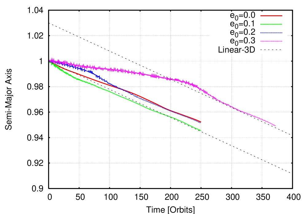
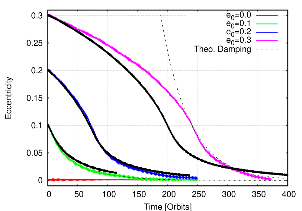
Figure 6: Top: Semi-major axis as a function of time for $q=6\times 10^{-5}$ in a 2D disk for different initial eccentricities. For very high eccentricities the speed of migration is significantly reduced as in the 3D case. Dashed lines indicate the result from linear analysis for 3D disks. Bottom: Eccentricity as a function of time for the same runs. The dashed lines indicate the linear results from Tanaka & Ward (2004) with $\tau_{ecc}=47$. Our 3D results are over-plotted using the small black symbols. For larger initial eccentricities 2D and 3D runs begin to differ; by about 20% for the $e_{0}=0.3$ case. Possible reasons for this behaviour are discussed in the text.

There are also some distinct differences. In the bottom panel of Fig. 6 the eccentricity is plotted as a function of time. Over-plotted (dashed curves) are the linear damping rates by Tanaka & Ward (2004), where our damping is again slightly faster. Our damping rates for the 2D and 3D cases agree very well for the smaller eccentricities while for the large value $e_{0}=0.3$ the 3D run gives a significantly faster damping. However, the generic features and scaling of the damping process for large $e_{0}$ is captured correctly in both 2D and 3D runs, and the differences in the eccentricity damping are at the 20% level even for the largest $e_{0}$.

To examine the origin of this discrepancy, we performed additional 2D and 3D models with larger disks, $0.25\leq r\leq 3.5$, while preserving grid resolution, to rule out the possibility that boundary effects are the cause. A small difference in eccentricity reduction was observed at the transition to linear damping, $de/dt\propto e$, with longer non-linear and shorter linear $e$-folding times than for our standard disk model, but the difference is only a few percent and not of the order observed in Fig. 6. Runs with enhanced damping at the radial boundaries to reduce reflections did not change the results considerably, some damping is clearly required however, to avoid unphysical influence due to the boundaries.

As a next step we analysed the role of potential softening in more detail. While the use of a larger softening ($\epsilon=0.6H$) to approximate 3D disk structure is a well-known approach in 2D modelling, for sufficiently eccentric orbits in which a large region of the disk is sampled, our results indicate that a simple prescription for potential softening may no longer be sufficient to obtain agreement between 2D and 3D simulations. This may be due in part to the fact that for highly eccentric orbits the planet is crossing the resonances that drive the disk-planet interaction, such that a strong sensitivity to the softening prescription is expected (Papaloizou & Larwood 2000). Further calculations that we have performed indicate that a considerably more complex prescription for softening the gravitational potential will be required if 2D models are to be constructed that agree with 3D models for both high and low orbital eccentricities. Clearly, a softening that is spatially fixed and does not vary with radius (which $H$ does in fact) will not be correct, a conclusion which applies to the 3D case as well in case the simulation is resolution limited. In our case at $r=1$ the standard grid resolution yields a diagonal length of $\Delta\approx 0.9R_{Hill}$ for one gridcell. The torque cutoff $r_{torq}$ should also scale with the radial distance of the planet from the star and not be a function of semi-major axis alone.

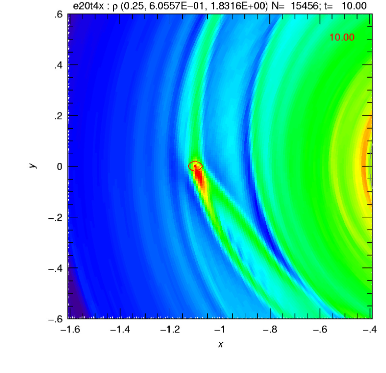
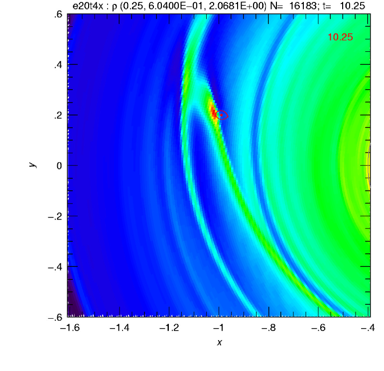
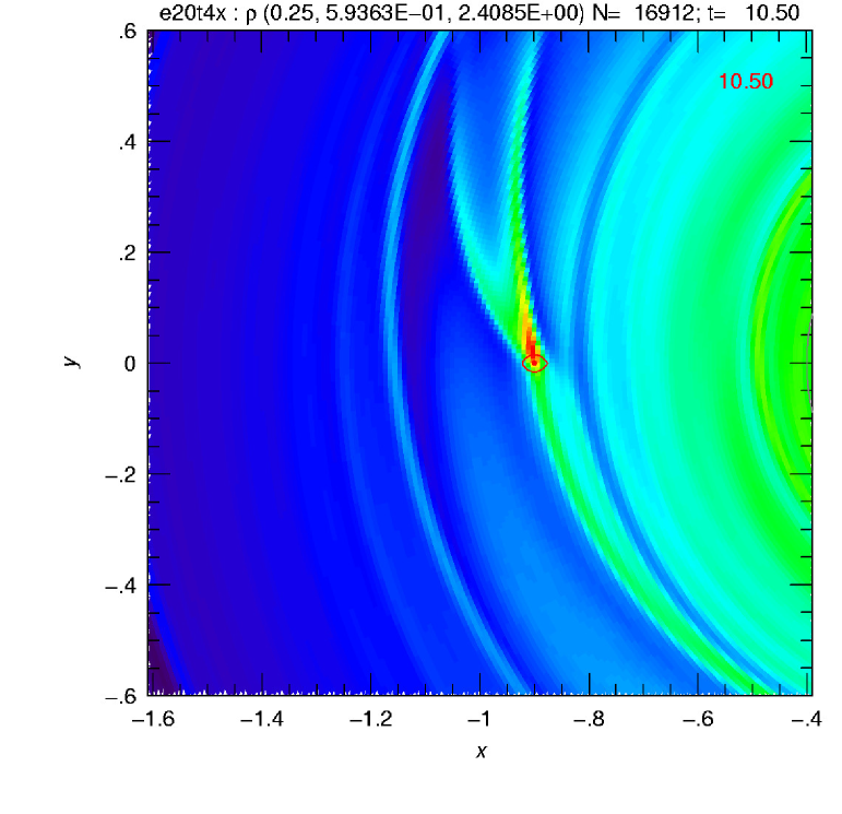
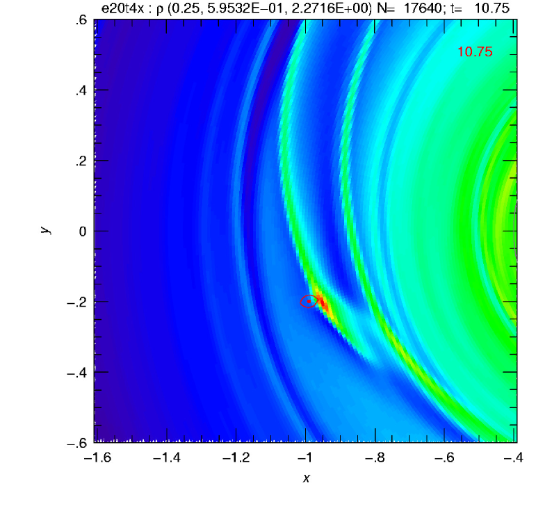
Figure 7: Density contour plot for a 20 Earth-mass planet on an fixed $e=0.1$ orbit imbedded in a 2D disk at four different times during one orbit. The snapshots are separated by 1/4 orbits.

We would like to point out that increasing the resolution of our models in the two- and three-dimensional case changes the time evolution of the semi-major axis only marginal, but lead to a slightly faster eccentricity damping. However, the observed discrepancy in timescales between the 2D and 3D case is not altered. See Appendix for a more detailed discussion on resolution issues.

3.4 Dynamics of the flow

To analyse the dynamical structure of the flow we consider the change of the flow field in the case of an eccentric planet for a 2D case. In Fig. 7 we display the density structure of the disk with an embedded $q=6\times 10^{-5}$ planet on an eccentric orbit with fixed $e=0.1$ at four different phases in the orbit, separated by 1/4 orbits, ranging from $t=10$ to $t=10.75$. At $t=10$ the planet is at apoastron (top left) and at $t=10.5$ at periastron (bottom left). In contrast to the evolution with zero eccentricity where two stationary trailing arms exist, one in the outer disk ($r>r_{p}$) and one in the inner disk ($r<r_{p}$), in this eccentric case spiral arms and additional flow features appear and disappear periodically in phase with the orbit. During periastron a pronounced outer spiral attached to the planet is visible while at apoastron this has changed to an inner spiral. This periodic shift of the spiral arm strengths will result in a corresponding periodic variation of the torque acting on the planet. We note also that a significant density enhancement appears in the close vicinity of the planet. At apoastron it clearly lies in front of the planet (and thus exerts a strong positive torque), and at periastron it lags behind the planet (exerting a strong negative torque). This flow feature appears to arise because when the orbit is eccentric the flow in the planet vicinity becomes similar to a Bondi-Hoyle flow. At apoastron the planet moves more slowly through the gas, and so is over-taken by the disk matter on trajectories that lie both inside and outside the planet orbit. These flow lines are distorted by the gravitational field of the planet and come to a focus in front of the planet, forming the high density feature seen in the top left panel of Fig. 7. The same effect happens in reverse at periastron, leading to a high density feature that forms behind the planet. These features become dominant in determining the torques experienced by the planet.

This is exemplified in Fig. 8 where we display the variation of the torque (see Eq. 9) acting on the planet and its radial distance form the star as a function of time for two different planetary eccentricities (top: $e=0.1$, and bottom: $e=0.3$). The top plot ($e=0.1$) refers directly to Fig. 7. Clearly in apoastron (strong inner spiral and leading high density feature) the total total torque is positive, while at periastron (strong outer spiral and lagging high density feature) the contribution is negative. Additionally there appears to be a small phase shift between the distance and the torques. Typically, for an embedded protoplanet the direction of migration and its magnitude is attributed to the sign and value of the torque acting on it. For the highly eccentric case ($e=0.3$) the average torque is clearly positive and one might expect outward migration.

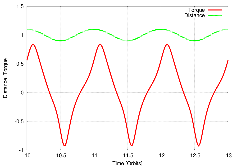
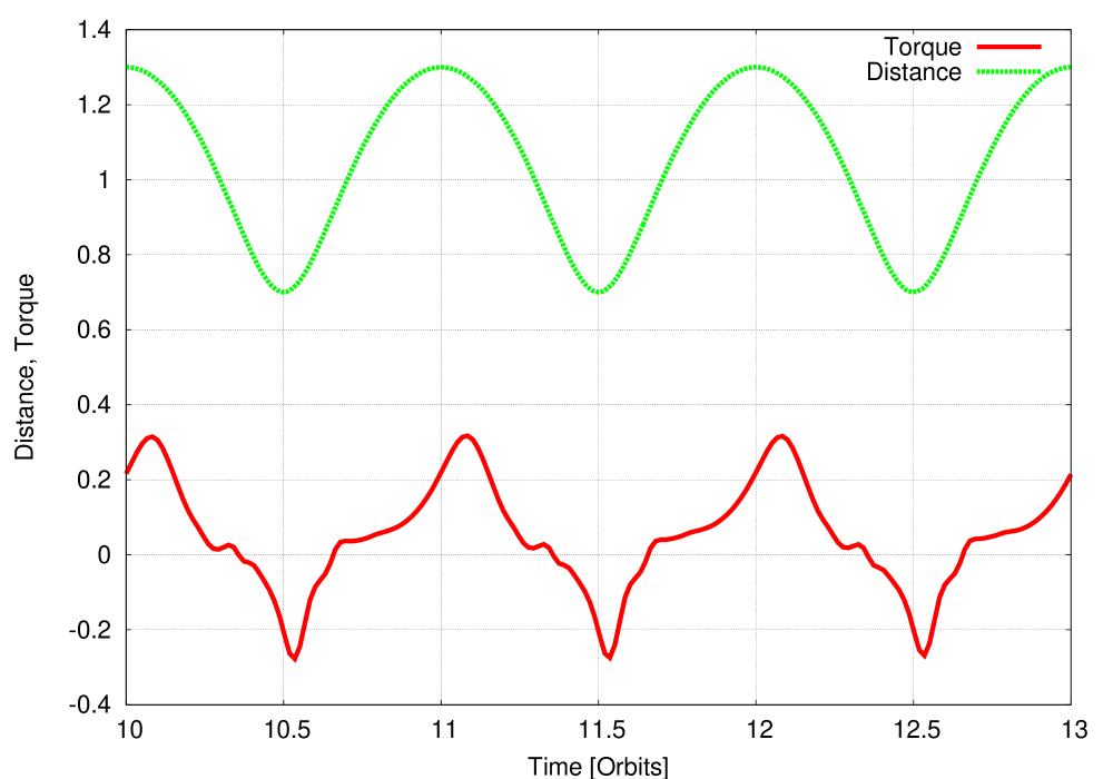
Figure 8: The change of the distance of the planet from the star and total disk torque acting on the planet as a function of time, where the torque is rescaled appropriately. The planet is held fixed on its orbit. Top: $e=0.1$ and Bottom: $e=0.3$.

However, this conclusion must be corrected for possible changes in the eccentricity of the planet. For a planet on an eccentric orbit its angular momentum $L_{\mathrm{p}}$ is given by

$$L_{\mathrm{p}}=m_{\mathrm{p}}\,\sqrt{GM_{*}a}\,\sqrt{1-e^{2}}$$ (7)

and the rate of change of the semi-major axis and eccentricity can be obtained from

$$\frac{\dot{L}_{\mathrm{p}}}{L_{\mathrm{p}}}=\frac{1}{2}\,\frac{\dot{a}}{a}-\frac{e^{2}}{1-e^{2}}\,\frac{\dot{e}}{e}\ =\,\frac{T_{\mathrm{disk}}}{L_{\mathrm{p}}}$$ (8)

Here $T_{\mathrm{disk}}$ is the total torque exerted by the disk onto the planet

$$T_{\mathrm{disk}}\,=\,\int_{Disk}\,\left.(\@vec{r}_{p}\times\@vec{F})\right|_{z}\,df$$ (9)

where $\@vec{r}_{p}$ denotes the radius vector from the star to the planet, $\@vec{F}$ the (gravitational) force per unit area between the planet and a disk element (at location $\@vec{r}$ from the star), and $df$ the surface element. Eq. (8) implies that a positive torque may also result in eccentricity damping rather than outward migration. From our simulations we are able to disentangle the different contributions.

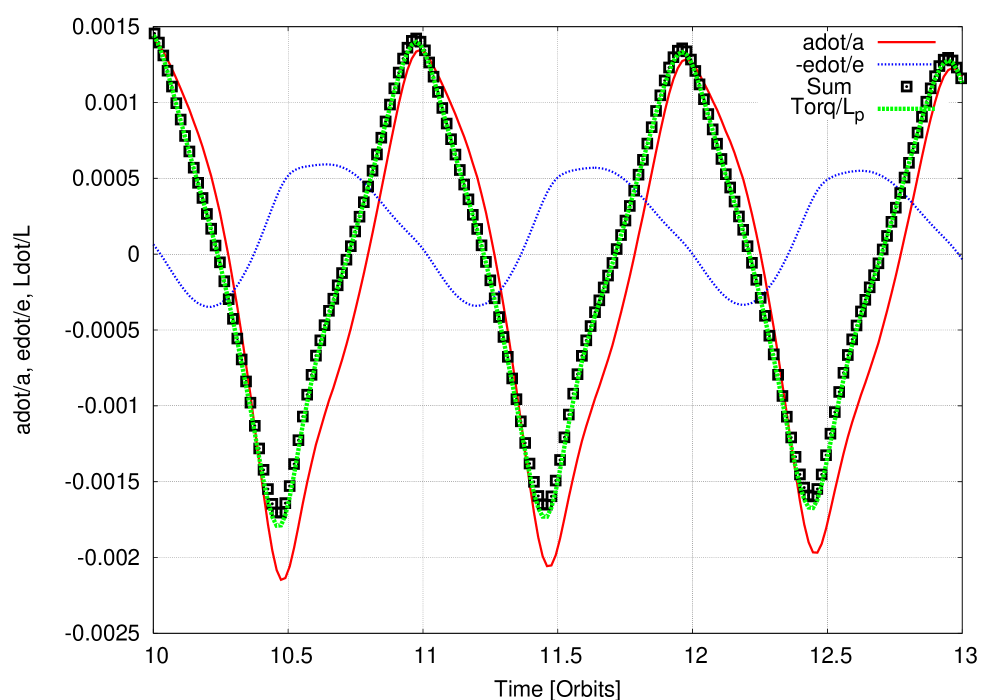
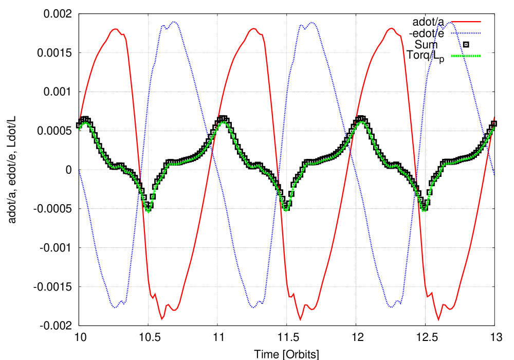
Figure 9: The time changes of the semi-major axis ($1/2\dot{a}/a$, solid curve), the eccentricity ($-e^{2}/(1-e^{2})\,\dot{e}/e$, thin dashed line), and the normalised torque ($T_{\mathrm{disk}}/L_{\mathrm{p}}$) for an evolving eccentric planet in a 2D disk. The sum of the first two contributions is given by the symbols. Top: $e_{0}=0.1$ and Bottom: $e_{0}=0.3$.

The evolution of the semi-major axis and eccentricity changes are displayed in Fig. 9 for two different initial eccentricities in the time interval 10 to 13 orbits. After this time the flow has equilibrated and the contribution of the individual terms in Eq. (8) can be analysed. In these calculations we have used a smoothed torque cutoff to reduce the noise in the curves. In both cases ($e_{0}=0.1$ and $e_{0}=0.3$) the sum of the two terms for $\dot{a}$ and $\dot{e}$ in Eq. (8) (thick dashed line) equals exactly the total disk torque as given by the squared symbols. The periodic behaviour of all quantities is again clearly visible, they all fluctuate around their zero value. Quite clearly, the contribution of the $\dot{e}$ term has comparable magnitude to the $\dot{a}$ value. Hence, a positive average total disk torque as for example in the $e=0.3$ case does not necessarily imply an outward migration of the planet, since the total torque is “shared” between semi-major axis and eccentricity change (see Eq. 8). A positive torque implies only that the angular momentum of the planet has to increase. For an eccentric orbit this can be achieved in two ways, either by increasing $a$ (outward migration) or by reducing $e$ (circularization). Indeed, for the semi-major axis to increase the planet’s total energy must increase. As described below, we find that it in fact decreases even though the angular momentum increases through the positive torque.

3.5 Migration rate

As noticed in the previous sections the migration rate depends on the eccentricity of the embedded planet and can vary by about 60% (cf. Fig. 4), an effect seen in the 2D as well as in the 3D simulations. For small eccentricities, that are less than or equal to about twice the disk aspect ratio ($e\leq 2H/r$), we find an increase in the migration rate. For larger values of $e$ the rate is reduced with respect to the circular case, but always directed inward. To analyse this effect we have performed additional simulations in 2D with varying eccentricities. To measure the values of the torque, the planet was held again on a fixed orbit.

In Fig. 10 we display the the evolution of the torque (top) and mechanical power (bottom) as a function of time over 2 orbital periods for different eccentricities. Here the energy change per time (power) of the planet due to the work done by the gravitational forces of the disk is given by

$$P_{\mathrm{disk}}\,=\,\int_{Disk}\,\@vec{r}_{\mathrm{p}}\cdot\@vec{F}\,df$$ (10)

The energy of the planet depends only on the semi-major axis $a$ and is given by

$$E_{\mathrm{p}}\,=\,-\,\frac{1}{2}\,\frac{GM_{*}m_{\mathrm{p}}}{a}$$ (11)

For the energy loss and semi-major axis change we then obtain

$$\frac{\dot{E}_{\mathrm{p}}}{|E_{\mathrm{p}}|}=\frac{\dot{a}}{a}\ =\,\frac{P_{\mathrm{disk}}}{|E_{\mathrm{p}}|}$$ (12)

Restriction to circular orbits with $e=0$ yields

$$\frac{\dot{E}_{\mathrm{p}}}{|E_{\mathrm{p}}|}=2\,\frac{\dot{L}_{\mathrm{p}}}{L_{\mathrm{p}}}$$ (13)

or for the normalized torque and power

$$\frac{P_{\mathrm{disk}}}{|E_{\mathrm{p}}|}=2\,\frac{T_{\mathrm{disk}}}{L_{\mathrm{p}}}$$ (14)

This relationship which can be directly verified from Fig. 10 where the normalised torque and energy loss is displayed as a function of time for various eccentricities. For low eccentricities ($e=0$: inverted triangles, $e=0.02$: open diamonds) the shape of the curves are in good agreement, and only scaled by a factor of 2. However, for eccentric non-circular motion this simple relation is not satisfied anymore.

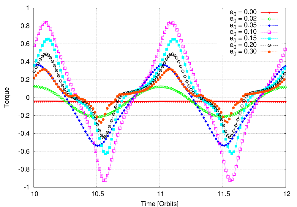
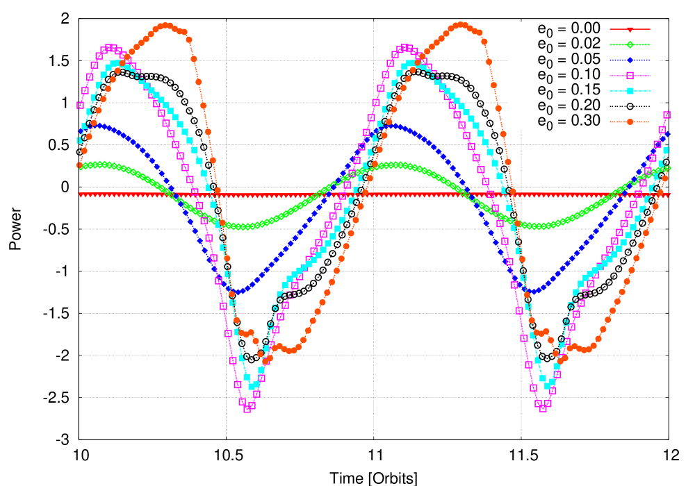
Figure 10: Top: Normalised Torque ($T_{\mathrm{disk}}/{L_{\mathrm{p}}}$) vs. time for various eccentricities, where the orbit is not allowed to evolve. Bottom: the corresponding energy loss ($P_{\mathrm{disk}}/{|E_{\mathrm{p}}|}$). The values have been amplified vertically by the same amount as in Fig. 8.

Already at very low eccentricities the variations of the power exceed the mean value for $e=0$ by a large margin. For zero eccentricity the value for the power is about -0.09 in the displayed units (solid curve with inverted triangles). For $e=0.02$ (light dashed curve with open diamonds) we find an amplitude of 0.37, and for $e=0.05$ (dark dashed curve with filled diamonds) it has increased to 1.00 (bottom plot in Fig. 10). Hence, a small asymmetry in the power may lead to a substantial change in the migration rate. From Fig. 10 it is clear that in particular during periapses ($t=10.5$ and $11.5$) the planets experiences a large energy loss which reaches a maximum for an eccentricity around $e=0.10$. As a consequence the mean value (of $P_{disk}$) has significantly dropped below the circular case, leading to the enhanced inward migration found previously. For larger $e$ the amplitude of the power variation remains approximately at the same value but becomes more symmetric, leading to a reduction in the migration rate. As the orbit–integrated power remains negative for the high eccentricity cases (i.e. $e\simeq 0.3$), the migration remains inward even though the orbit integrated torque is positive.

The variation of the torque for non-vanishing eccentricities also increases substantially above the zero eccentricity value (Fig. 10 top panel). Here, for larger values of $e$ above about $e=0.1$ the mean value becomes clearly positive. However, due to the corresponding change in eccentricity and energy the migration is still directed inwards (cf. Figs. 8 and 9).

To illuminate this effect from a different perspective we have performed a set of simulations where the planet was not allowed to move and remained on a fixed orbit during the simulations. We used 22 different values for the eccentricity ranging from $e=0$ to $e=0.40$ and ran all models up to a final time of 100 orbits where the torques and the power acting on the planet have reached an equilibrium on average. For the last 20 orbits (from $t=80$ to $100$) we calculate the time average of $T_{\mathrm{disk}}$ and $P_{\mathrm{disk}}$. All these models are performed using the two-dimensional setup and utilize a $256\times 700$ grid with a logarithmic spacing in the radial direction. Additionally, to increase performance the runs use the FARGO-algorithm for differentially rotating flows (Masset 2000). The results are displayed in Fig. 11 where the inverted triangles refer to the torque and the solid dots to the power acting on the planet, both given in dimensionless units. Clearly, as already found through the previous analysis an increase in the eccentricity leads to a non-monotonic behaviour of both $T_{\mathrm{disk}}$ and $P_{\mathrm{disk}}$. For circular motion both are identical and negative, leading the the well known inward migration of the planet. Upon increasing the eccentricity both quantities initially drop even more and increase later again. The power remains negative for all eccentricities leading to the inward migration which only slows down for larger $e$. This leads to the behaviour of migration time scales as shown in Fig. 4 above, which are shortest for $e\approx 0.08$. The torque becomes positive for all $e>0.08$ and reaches a maximum for $e\approx 0.17$.

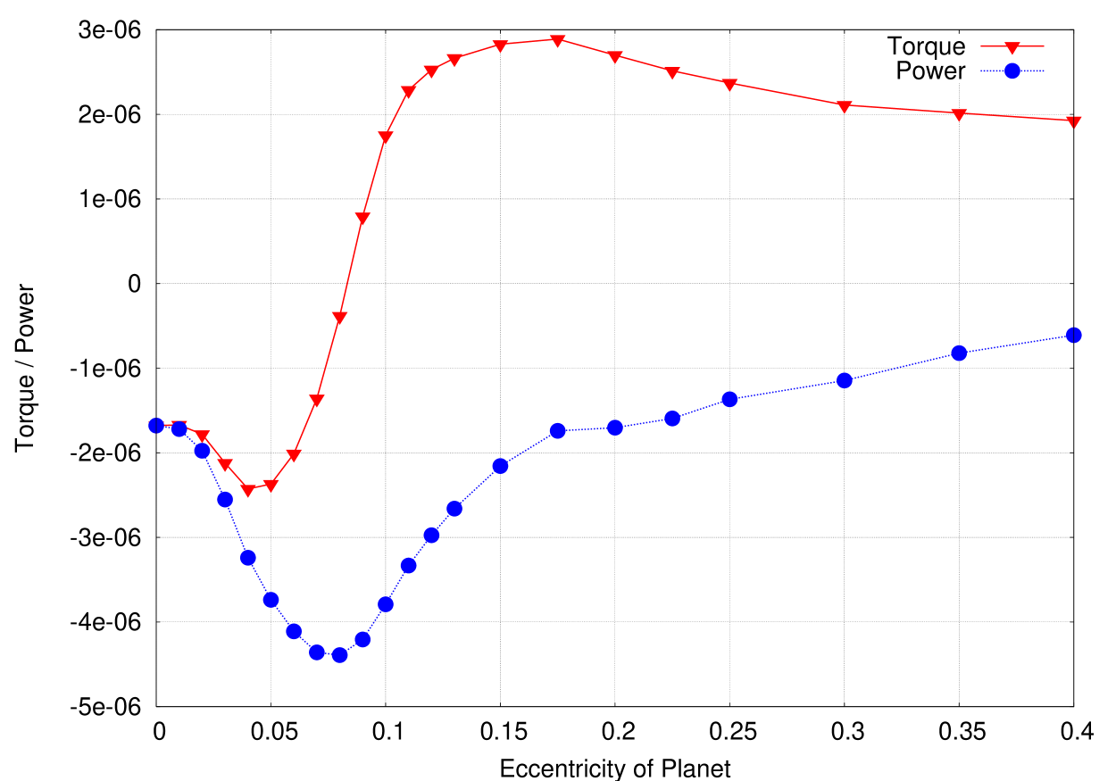
Figure 11: Dimensionless torque ($T_{\mathrm{disk}}$) and energy loss (power, $P_{\mathrm{disk}}$) experienced by the planet for different eccentricities. The values are obtained by keeping the planet on a fixed orbit and using time averages over 20 orbits (from $t=80$ to $100$).

3.6 Changing the disk’s density profile

All the previous simulations have been peformed using a surface density profile which varies as $\Sigma(r)\propto r^{-p}$, where we used $p=1/2$ which is the equilibrium profile for a constant kinematic viscosity and closed radial boundaries ($\dot{M}=0$). The corotation torques acting on the planet and the resulting changes in migration speed depend (for circular orbits) on the density slope of the disk (Tanaka et al. 2002; Masset et al. 2006). To test the possible influence of the density slope on the orbital evolution of eccentric (non-inclined) planets, we have varied the value of $p$ from 0 to 1.5 for our highest value of the eccentricity, $e=0.3$. The results of our simulations are displayed in Fig. 12. For an increasing density slope the migration occurs monotonically at a faster rate, in agreement with standard linear estimates for the torques (Tanaka et al. 2002). The eccentricity evolution is much less affected, the largest change occurs only for the steepest slope $p=1.5$. These results indicate that in the case of eccentric planets the importance of the corotation torques are greatly reduced. This is probably because during each orbit, the planet moves a distance radially that is larger than the width of the horseshoe region, where the corotation torque is generated. Clearly it is expected that the corotation torque will weaken significantly under these conditions. In all four cases with different $p$ the average torque is clearly positive while the power is negative. As in the previous $p=1/2$ case this leads to inward migration and eccentricity damping. In particular our results concerning the positive torque are in agreement with the earlier findings of Papaloizou & Larwood (2000) who used $p=1.5$, but fixed the planetary orbit and did not measure the power.

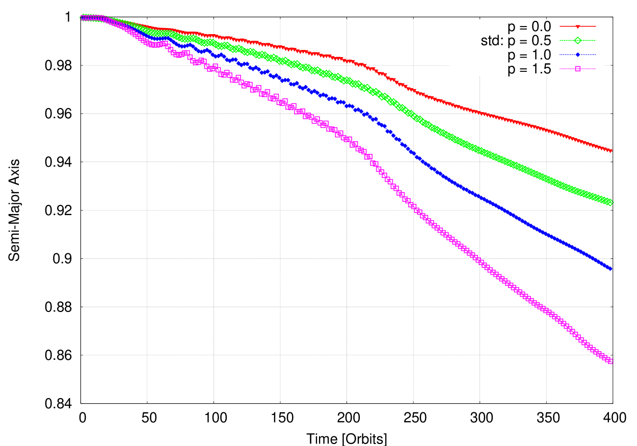
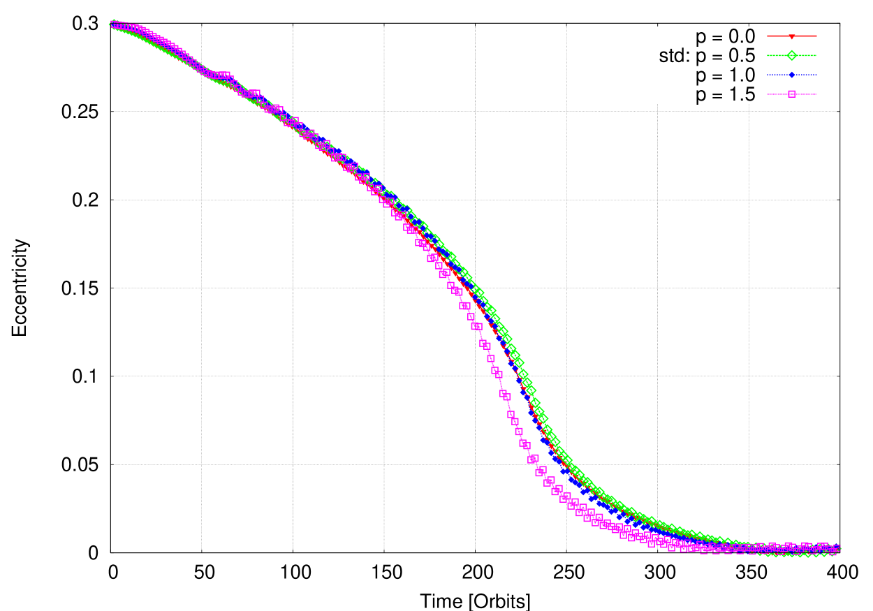
Figure 12: Top: Time-change in semi-major axis for different surface density profils of the disk, given by $\Sigma(r)\propto r^{-p}$. Bottom: Corresponding eccentricity evolution.

4 Inclined orbits

In addition to the eccentric planetary orbits we now study the additional degree of freedom provided by inclined orbits. We begin by considering inclined, circular orbits, before discussing the general case when both $e$ and $i$ are non-vanishing initially.

4.1 Circular Orbit

If we start a low mass planet on a circular but inclined orbit the orbital inclination will be damped (cf. Fig. 13). For $i\simeq e$, the time scale for inclination damping is somewhat longer than for the eccentricity damping, but of the same order of magnitude. Again we find two different regimes. For $i<H/r$ ($i$ in radians) the planet remains inside the main body of the disk and the damping is exponential: $di/dt\propto i$. The damping rate (averaged over one planetary orbit) for a small planet mass and small inclinations is obtained through linear calculations by Tanaka & Ward (2004) as

$$\frac{\overline{di/dt}}{i}\,=\frac{1}{\tau_{inc}}\,=-\frac{0.544}{t_{wave}}$$ (15)

with $t_{wave}$ defined in equation (5). For our simulations this gives an inclination damping time scale $\tau_{inc}$ of about 68 orbits. The two lower curves in the upper panel of Fig. 13 show the inclination damping for small initial inclinations (2^∘ and 5^∘ respectively). The fitted dashed line for $i_{0}=2^{\circ}$ corresponds to an exponential damping with a timescale of 90 orbits. This obtained $\tau_{inc}$ is larger than the linear estimate (Tanaka & Ward 2004) by the same factor as the eccentricity damping time $\tau_{ecc}$.

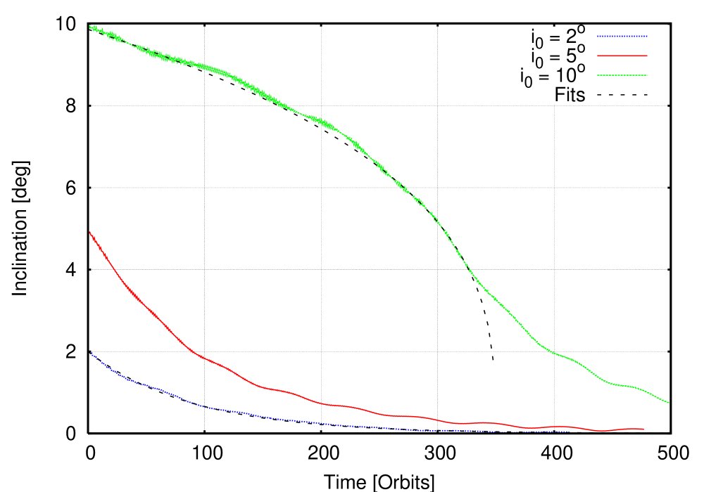
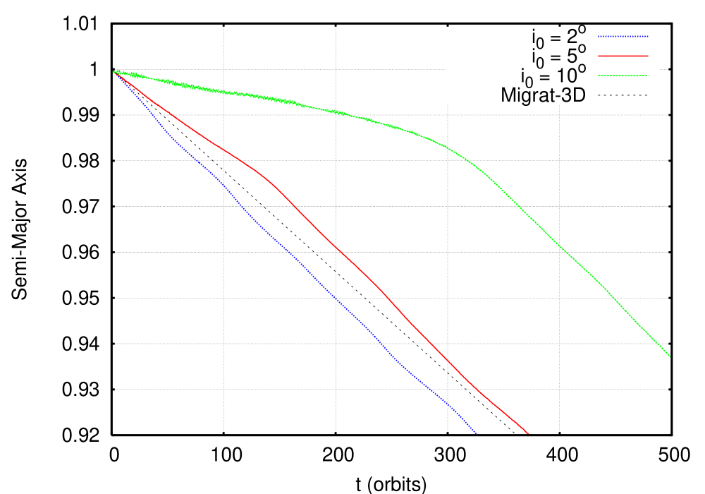
Figure 13: Orbital inclination (top panel) and semi-major axis (lower panel) as a function of time for different initial values of $i$ for a 20 Earth-mass planet on a circular orbit. We find exponential decay of $i$ as long as $i\leq 6^{\circ}$; the thin dashed line superimposed on the lowest $i_{0}=2^{\circ}$ curve corresponds to an exponential with a damping timescale $\tau_{inc}=90$. For higher inclinations the damping timescale increases dramatically. A very good fit is found for a model with $di/dt\propto i^{-2}$ (thin dashed line for $i_{0}=10^{\circ}$).

For higher inclinations we find a slower inclination damping rate as can be seen in Fig. 13 for $i_{0}=10^{\circ}$. For our disk parameters, the damping rate departs from being exponential for values of $i$ in the interval 6${}^{\circ}<i<8^{\circ}$. Just as for the damping of eccentricities, we therefore find that the linear calculations of Tanaka & Ward (2004) provide a good approximation for over twice their formal range of applicability, i.e.  up to $i\sim 2H/r$ - where here $i$ is measured in radians. For $i\geq 8^{\circ}$ the damping rate strongly deviates from being exponential, and the best fit to the model with the highest initial inclination of 10^∘ is given by $di/dt\propto i^{-2}$ (upper dashed line in Fig. 13). Interestingly, this dependency is identical to the behaviour of the eccentricity damping for large eccentricities. However, here the reduced damping comes from the fact that for inclinations significantly larger than $H/r$ the planet’s contact with the disk is reduced, and its velocity relative to local disk gas as it crosses the midplane is increased.

As with increasingly eccentric planar orbits, the migration rate is observed to decrease with increased inclination, as shown in Fig. 13 (lower panel). The effect of an increased inclination is weaker than for a comparable value of eccentricity: circular, inclined orbits lead only to weaker torques on the planet, and not the possibility of torque sign reversal. Migration rates return smoothly to values close to the planar, circular rate once the inclination drops beneath about 5^∘.

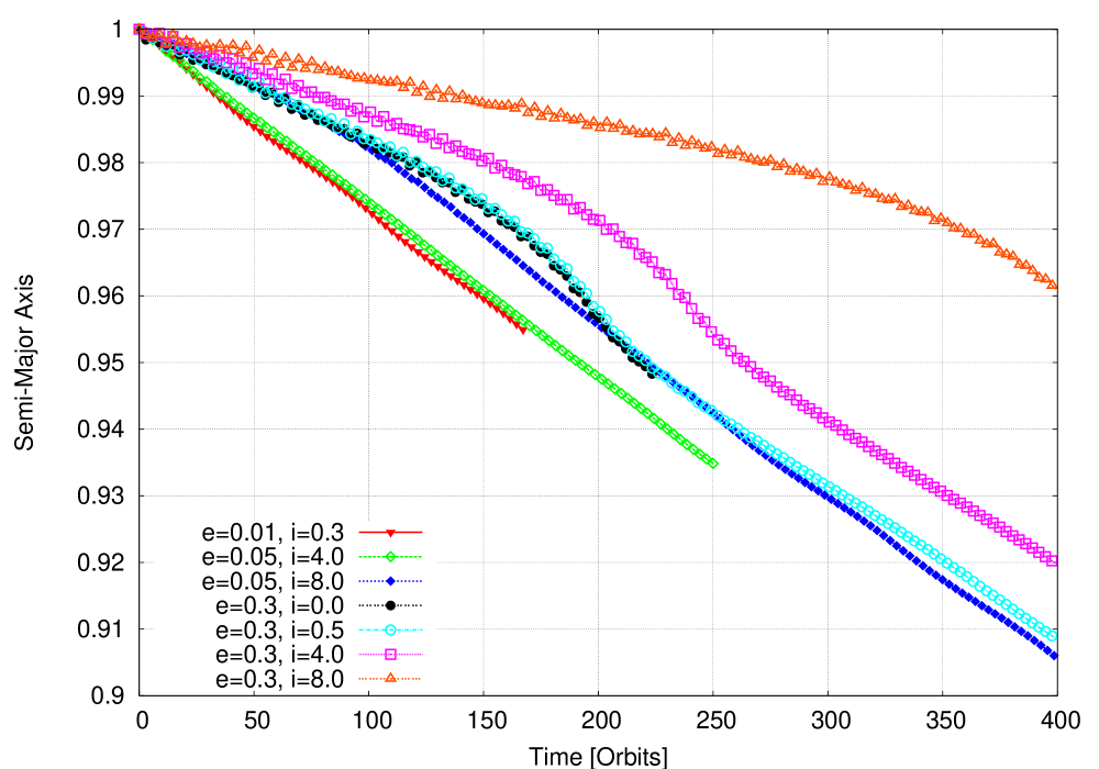
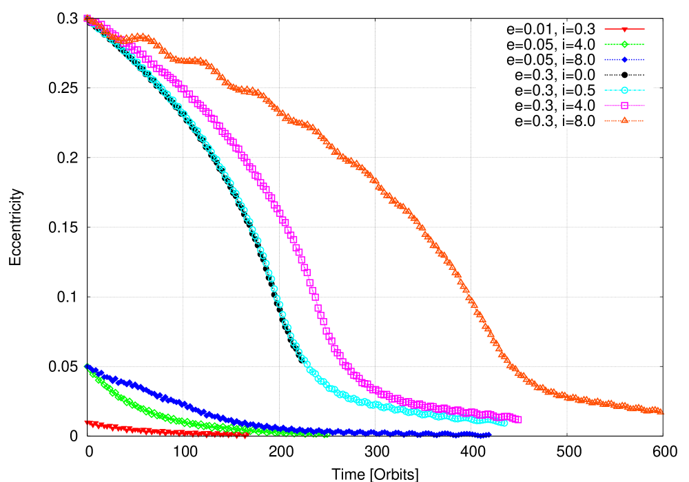
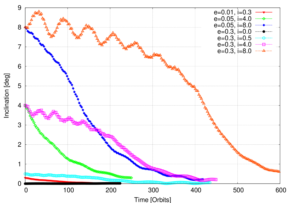
Figure 14: Semi-major axis, eccentricity and inclination as a function of time for a 20 $m_{E}$ planet with different initial eccentricities and inclinations. In the top panel the time coordinate has been stretched to show effects more clearly.

4.2 Non-circular Orbits

Finally we investigate several models in which both the initial eccentricity and the initial inclination are nonzero with $0<e_{0}<0.30$ and $0<i_{0}<8^{\circ}$. Each system was initialised with the planet at apocentre above the midplane, with the longitude of pericentre $\omega=\pi/2$. Our results are summarised in Fig. 14.

4.2.1 Small $e$ and small $i$

We begin by considering the evolution of orbits for which the planets are initiated to have small values of eccentricity and inclination (i.e. $e_{0}\lesssim H/R$ and $i_{0}\lesssim H/R$, where $i_{0}$ is measured in radians).

Examining the top panel of Fig. 14 we can see the migration behaviour for runs with ($e_{0}=0.01$ and $i_{0}=0.3^{\circ}$) and ($e_{0}=0.05$ and $i_{0}=4^{\circ}$). It is clear that for small values of both $e_{0}$ and $i_{0}$ the migration behaves as if the orbit was essentially uninclined. Small values of the inclination such that $i\leq H/R$, with $i$ measured in radians, cause migration to be slowed, but only very slightly.

Examining the middle panel of Fig. 14, we can see that small values of $e_{0}$ and $i_{0}$ lead to exponential decay of the planet eccentricity, with the rate of damping only slightly increased by the small inclination. Examining Fig. 1 we see that the time taken for the $e_{0}=0.1$ case to halve its eccentricity is $\simeq 35$ orbits, and the time required for the $e_{0}=0.05$, $i_{0}=4^{\circ}$ case shown in Fig. 14 to also halve its eccentricity is approximately 40 orbits.

The lowest panel in Fig. 14 shows the inclination evolution. In common with the eccentricity damping, we find that the inclination damping for an orbit with small initial values of $e$ and $i$ occurs exponentially on a time scale very similar to the case when the orbit is circular but inclined.

4.2.2 Small $i$ and large $e$

We now consider the orbital evolution when the inclination is small ($i\lesssim H/R$) and the eccentricity is large ($e>H/R$). This is represented by the runs shown in Fig. 14 with ($e_{0}=0.3$ and $i_{0}=0.5^{\circ}$) and ($e_{0}=0.3$ and $i_{0}=4^{\circ}$). Also shown for reference is a case with ($e_{0}=0.3$ and $i_{0}=0$). The migration is shown in the top panel. We have already shown in previous sections that an uninclined, high eccentricity orbit undergoes slower inward migration than a circular orbit does. We see that increasing the inclination increases the migration time further. A very small inclination ($i=0.5^{\circ}$) has very little effect, but an inclination of $i=4^{\circ}$ begins to make a noticeable difference, decreasing the migration rate by $\simeq 25\%$.

The eccentricity evolution of these runs is shown in the middle panel of Fig. 14. The discussion presented in previous sections showed that an uninclined, highly eccentric orbit shows an eccentricity decay rate $de/dt\propto e^{-2}$. We can see that a very small inclination ($i=0.5^{\circ}$) has essentially no effect, but an inclination of $i=4^{\circ}$ extends the damping time by about 25%, while preserving the shape of the curve of $e$ versus time.

The inclination evolution is shown in the lowest panel. If we consider the evolution of the runs with $i_{0}=4^{\circ}$, then we see a fairly dramatic change in the inclination damping once $e_{0}>>H/R$. For small values of $e_{0}$ we see the usual exponential decline of $i$. When $e_{0}$ is large, however, the inclination damping rate is small (even for small inclination) and almost constant with superimposed oscillations until the eccentricity falls below $e\simeq 0.1$, after which it recovers the exponential decay. For example, the $i_{0}=4^{\circ}$ and $e_{0}=0.3$ case shows an inclination decay time scale $i_{0}/(di/dt)\sim 700$ orbits initially. Once the eccentricity has damped to $e\leq 0.1$ after approximately 200 orbits, the inclination declines exponentially on an e-folding timescale of $\simeq 90$ orbits. The period of the oscillations seen in the inclination corresponds approximately to the precession period of the nodal line of the planet.

4.2.3 Large $i$ and small $e$

We now consider the evolution when the inclination $i$ is large and the eccentricity is small, which is represented in Fig. 14 by the run with ($i_{0}=8^{\circ}$ and $e_{0}=0.05$). The migration is shown in the top panel, and we can see that compared to the run with ($i_{0}=4^{\circ}$ and $e_{0}=0.05$) the migration rate for the more inclined planet is slower by about 40%, such that a doubling of the initial inclination leads to a migration rate that is almost halved. After just over 220 orbits the migration rate approaches that for uninclined orbits as the inclination has decreased sufficiently after this time.

The eccentricity evolution for this run is shown in the middle panel of Fig. 14. Comparing this run with the one with ($i_{0}=4^{\circ}$ and $e_{0}=0.05$) we see that having a large inclination substantially increases the damping time. Close to the beginning of the simulation the low inclination run has its eccentricity reduced by about 50% within $\simeq 40$ orbits, whereas the more inclined run shows only a 20% change in eccentricity after this time. The damping of eccentricity also shows a strong deviation from exponential decay for the high inclination run, with the eccentricity decay rate being almost constant until the inclination has damped down to $\simeq 4^{\circ}$. Once the inclination has declined down to this value the eccentricity decay becomes exponential.

We have already discussed the inclination evolution for circular orbits, and have shown that for large values of $i$ the inclination damping rate is no longer exponential, but scales as $di/dt\propto i^{-2}$. The addition of a small eccentricity ($e_{0}=0.05$) barely changes the decay rate for large inclinations, as shown in the lowest panel of Fig. 14. The effect of this small eccentricity is simply to lengthen the damping time by about $10\%$.

4.2.4 Large $i$ and large $e$

We now consider the evolution of orbits with both large inclination and eccentricity. The run with ($e_{0}=0.3$ and $i=8^{\circ}$), plotted in Fig. 14 illustrates this case. The migration rate, shown in the top panel, is seen to be reduced substantially compared to both the cases with ($e_{0}=0.3$ and $i_{0}=4^{\circ}$), and ($e_{0}=0.05$ and $i_{0}=8^{\circ}$). An increase of inclination from $4^{\circ}$ to $8^{\circ}$, with eccentricity $e=0.3$ leads to a $\simeq 50\%$ reduction in the initial migration rate. However, we note that the rapid damping of inclination and eccentricity means that this reduction in migration rate is short lived, and can at most only increase the total migration time through the disk by $<10\%$ in the absence of a mechanism to maintain $e$ and $i$ at large values (Cresswell & Nelson 2006).

The eccentricity evolution shown in the middle panel demonstrates that when $e_{0}=0.3$, increasing the inclination from $4^{\circ}$ to $8^{\circ}$ causes a significant lengthening of the initial eccentricity damping time (by about a factor of 2). As for the other high eccentricity/inclination runs, the damping is no longer exponential while $e>0.1$ or $i>4^{\circ}$, but becomes so once the eccentricity and inclination fall beneath these values.

The inclination damping shows similar behaviour to the eccentricity damping for this large $e$ and $i$ run, although the dependence of $di/dt$ on $i$ is slightly weaker than that seen for $de/dt$. Increasing the inclination from $i=4^{\circ}$ to $i=8^{\circ}$ with $e_{0}=0.3$ decreases the initial inclination damping rate by about 40%, with little change to the overall shape of the curve. We see that both the eccentricity and inclination decay on similar time scales (within about 300 orbits for $e$ and 350 orbits for $i$), and once they have reached small values they under go exponential decay toward zero.

5 Conclusions

We have performed fully non-linear 2- and 3-dimensional hydrodynamical simulations of a planet embedded in a protoplanetary disk. The planet was allowed to change its orbit due to the torques from the disk material. We investigated the orbital evolution of the planet in the linear low mass regime (Type I migration) for which analytical studies of the eccentricity and inclination damping rates are known.

Concerning the damping of eccentricities and inclinations, for small values $e<0.1$ and $i<5^{\circ}$ we find very good agreement between our non-linear results and existing linear theory (Tanaka & Ward 2004). The damping occurs for both, $i$ and $e$, exponentially with a time scale $\tau\propto(H/r)^{2}\tau_{mig}$. The quantitative agreement of our numerical results with the estimates of the linear calculations for the eccentricity and inclination damping are at the 20-30% level, which is very encouraging considering that one always has to use both gravitational smoothing and torque–cutoff within the planet Hill sphere in numerical simulations. Papaloizou & Larwood (2000) have shown through linear calculations that the absolute magnitude of the torque depends on the value of the gravitational smoothing $\epsilon$, and the slightly longer damping times that we find in 3D simulations is probably an indication that softening is playing a role. In addition, Masset et al. (2006) have suggested that departures from the linear results may occur for 20 Earth mass planets that we have considered, so we should probably not expect perfect agreement with the results of Tanaka & Ward (2004).

For our adopted $H/r=0.05$, the critical values for $e$ and $i$ (in radians) lie approximately at $2H/r$. Above those critical values the time behaviour changes for both, eccentricity and inclination. In both cases we find a damping following $dy/dt\propto y^{-2}$ with $y\in\{e,i\}$, which (for the eccentricity) has been suggested recently by Papaloizou & Larwood (2000). For the inclination we attribute this behaviour to the fact that on highly inclined orbits the planet loses contact with the disk and experiences only reduced damping, while for the eccentricity it is has been attributed to the varying planetary velocity with respect to the disk material (Papaloizou & Larwood 2000).

For the migration rates as a function of eccentricity we find some surprising results: For low eccentricities in the exponential damping regime we find faster migration than in the case of zero eccentricity - an increase of up to 60% is observed. Through a detailed analysis of torque and energy loss balance during the planetary orbit we attribute this increased migration rate to an increase in the energy loss during periapse of the planet which reaches a maximum at $e\approx 0.1$. For larger eccentricities the migration rate is reduced significantly below the circular case but is still directed inward even for $e=0.3$, even though the average torques are clearly positive. Migration can still be inward in this case because the torque largely goes into damping of the eccentricity while the planet continues to lose energy on average. If a situation were to arise where this energy loss could be compensated for, for example by gravitational interaction with surrounding planets, then in principle the positive disc torque could drive outward migration. Simulations by Cresswell & Nelson (2006) have explored this possibility, but find that eventually the eccentricity of all planets damps and inward migration of the planetary swarm occurs.

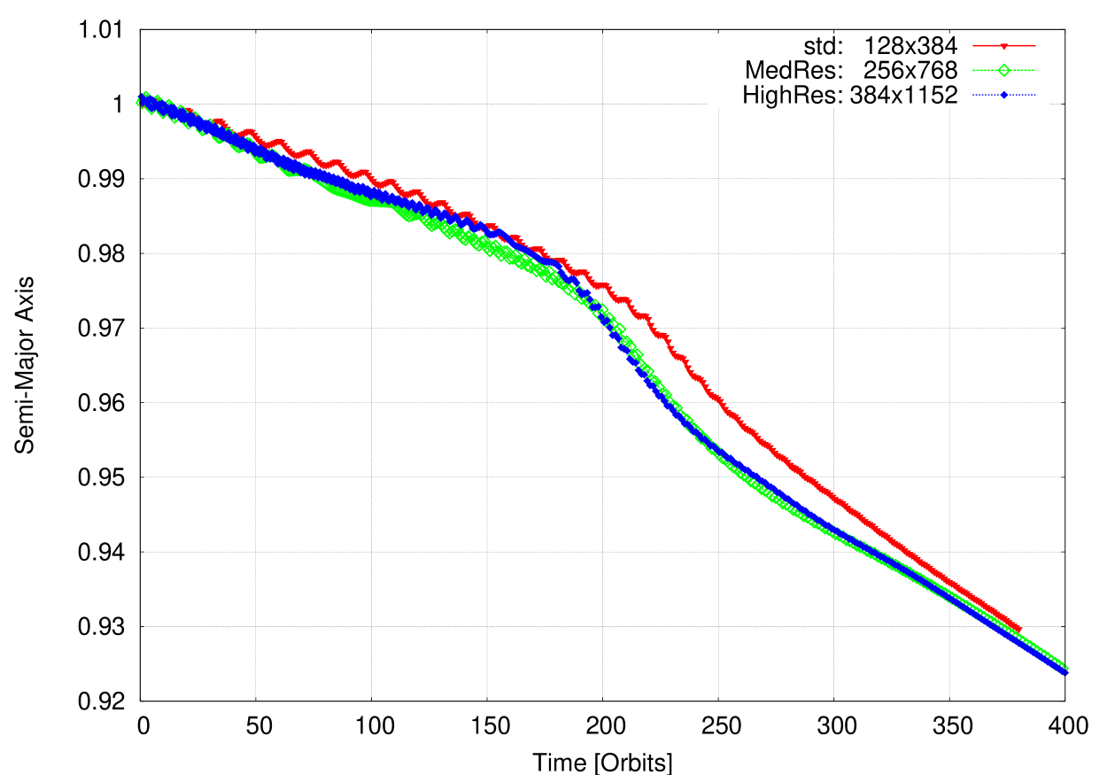
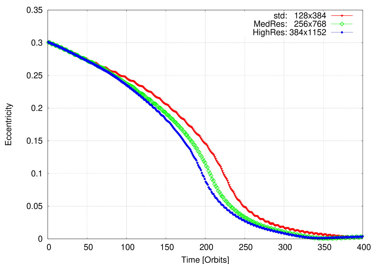
Figure 15: Semi-major axis and eccentricity as a function of time for a two-dimensional disk with a 20 $m_{E}$ planet and an initial eccentricity $e_{0}=0.3$ for different grid resolutions.

We compare our 3D results in detail with corresponding 2D simulations in the case of vanishing inclinations. For coplanar orbits and small eccentricities the results of the 2D and 3D simulations are in excellent agreement with respect to the migration rate and the eccentricity damping time scale. The increased migration for small non-zero eccentricities is also reproduced. For eccentricities $e>0.25$, agreement between the 2D and 3D is poorer. While the qualitative behaviour is still very similar, we find differences in the time scales. For example, the eccentricity damping rate between 2D and 3D differs by 10-20% for the $e_{0}=0.3$ case. As the planet samples a large range of cell sizes and the interaction becomes more sensitive to the smoothing length selected. This issue can be solved if detailed knowledge of the problem under examination is known beforehand, but with the increased availability of high-performance and parallel computing facilities, it is questionable as to whether the results are worth the investment. Hence, the evolution of embedded planets can be studied in 2D, for eccentricities of up to several scaleheights, if the right smoothing length is chosen for the potential. For larger values of eccentricity, $e$-folding times are typically overestimated.

For the combined general case, non-zero eccentricity and inclined orbits, we find that provided the eccentricity or inclination remains small, the previous formulae remain a good approximation of a planet’s behaviour. Inclination produces a weaker departure from the circular, planar case than the same value of eccentricity, and non-linear effects set in sooner for lower $e$ when both parameters are non-zero. The migration rate may be moderately (factors of $\sim$ 2 – 3) reduced if both $e$ and $i$ are towards the upper limits of this range. Once both parameters enter the non-linear regime however, cross-terms become significant in both the damping and migration, and the previous correspondences ($de/dt\propto e^{-2},di/dt\propto i^{-2}$) are lost. Secular effects from the disk can lead to moderate, short-term oscillations in $e$ and $i$.

Our results indicate that the interaction of a small mass planet (here 20 $m_{E}$) with its protoplanetary disk always leads to a rapid damping of its eccentricity and inclination. Additionally, the main effects and timescales are captured very well by a two-dimensional approach which greatly simplifies the computational effort. Only if additional perturbers, such as other planets or a stellar binary companion, are present may the eccentricity/inclination of the planet and the disk be excited.

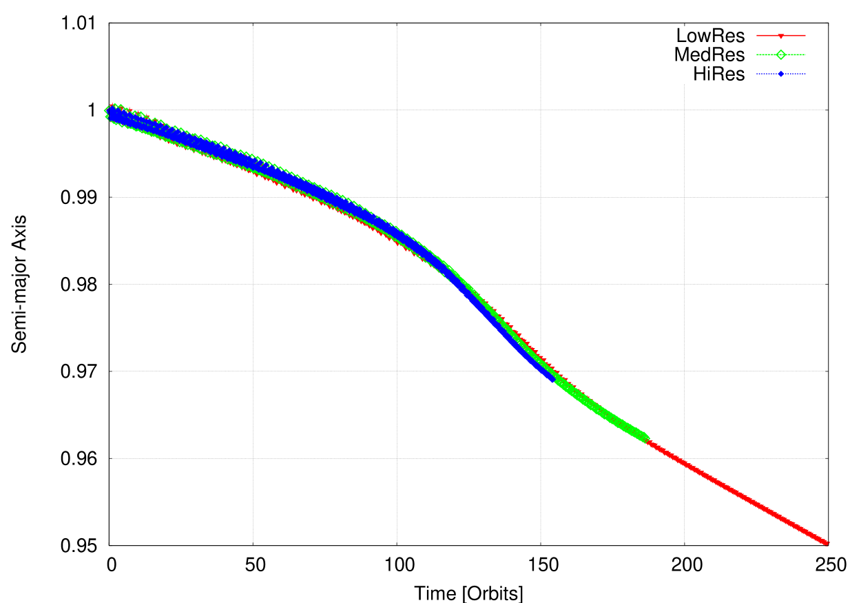
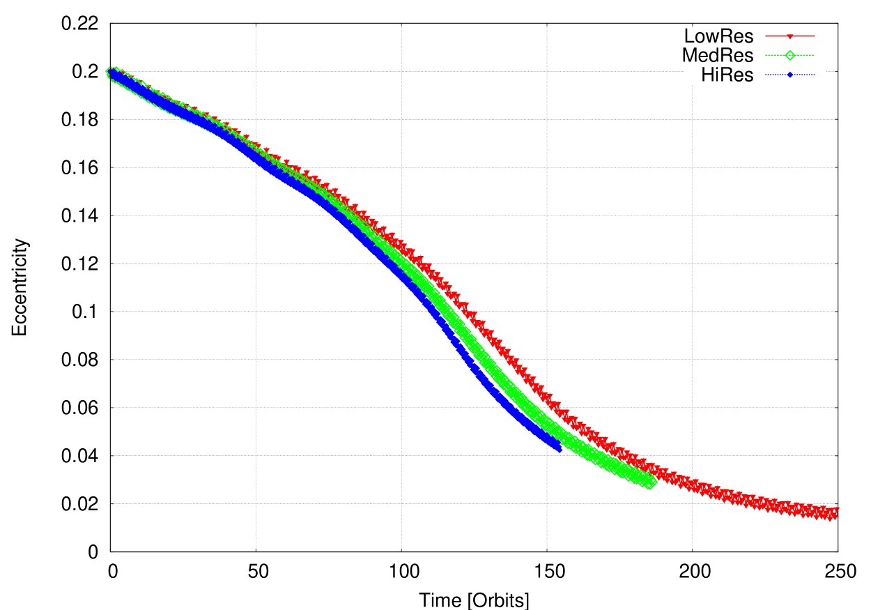
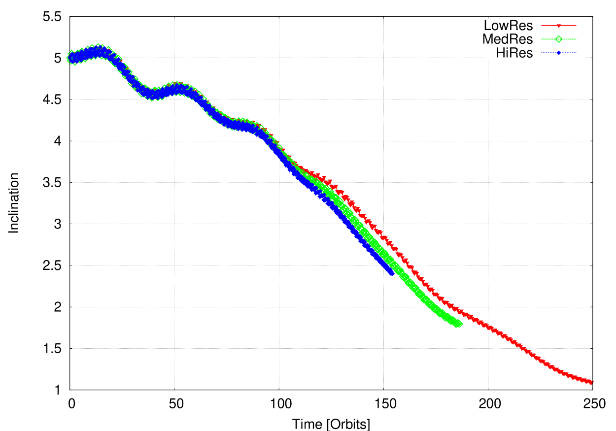
Figure 16: Semi-major axis, eccentricity and inclination as a function of time for a 20 $m_{E}$ planet in a three-dimensional disk, for different grid resolutions (see text).

Appendix A Numerical convergence

To test the issue of numerical convergence we have run a subset of the previously described models with a higher grid resolution. In all simulations we use a torque cutoff of $r_{torq}=0.8R_{Hill}$ and (in the 3D cases) a smoothing length of identical extension.

The first set of simulations refer to the two-dimensonal setup (2D-disks). From our standard resolution in 2D with $N_{r}\times N_{\varphi}=128\times 384$ we first doubled the number of gridpoints in each dimenension to a medium resolution of $256\times 768$ and then increased it by again a factor of $\sqrt{2}=1.41$ to $384\times 1152$, our high resolution case. The results for an initial eccentricity of $e_{0}=0.3$, as displayed in Fig. 15, indicate first a qualitatively identical behaviour for all cases, with only a minor shortening of the eccentricity damping timescale with higher resolution, which amounts to about 15% difference in $\tau_{e}$ between the standard and the HiRes case. The differences in the migration can be attributed to the changing eccentricity damping, as in the initial phase of the evolution the migration rate is nearly identical for all three models. By chosing the highest value for the eccentricity we intended to pick out the most extreme case, and we expect the variations to be smaller for lower eccentricities.

Running a set of three-dimensional simulations on a typical parameter set with $e_{0}=0.2,i_{0}=5^{\circ}$ with obtain the results displayed in Fig. 16. Here, low resolution refers to $(N_{r},N_{\theta},N_{\varphi})=(132,40,390)$, medium resolution to $(N_{r},N_{\theta},N_{\varphi})=(184,56,560)$ and high resolution to $(N_{r},N_{\theta},N_{\varphi})=(264,80,800)$, i.e. the three cases differ by about a factor of $\sqrt{2}$ in the number of grid cells in each dimension, which gives about a factor of 16 in computation time between the highest and lowest resolution. The results are very similar to the 2D case for the eccentricity and migration. The eccentricity damping time scale shortens slightly (by about 10 %) when comparing the highest and lowest resolution runs, while the migration rate hardly changes at all. The inclination damping time shortens as well upon increasing the resolution (Fig. 16), but this is largely a result of the change in eccentricity damping time (see below). Additional resolution studies performed in 3D for $e_{0}=0.2,i_{0}=0$ and $e_{0}=0,i_{0}=5$ yielded very similar results and are not shown here. In the case with $e_{0}=0,i_{0}=5$ degrees, we found that the inclination damping time was hardly affected by the changes in resolution, which is why the deviation in inclination damping times shown in fig. A.2 is actually due to changes in the eccentricity damping time.

Both 2D and 3D resolution studies indicate that there are still residual changes at the 10 % level when the resolution changes, and this change mainly occurs in the eccentricity damping rate. Altogether our results demonstrate very clearly that the effect of an increased migration and inclination damping for larger $e$ and $i$ in a locally isothermal disc is a robust effect independent on resolution. The absolute magnitude will depend on physical details in the vicinity of the planet, where physics that we have not included in our models (e.g. thermal and radiative effects, MHD turbulence) will play a role amongst others (Nelson & Papaloizou 2004; Nelson 2005; Paardekooper & Mellema 2006)

References

- Artymowicz (1993) Artymowicz, P. 1993, ApJ, 419, 166
- Bate et al. (2003) Bate, M. R., Lubow, S. H., Ogilvie, G. I., & Miller, K. A. 2003, MNRAS, 341, 213
- Bryden et al. (1999) Bryden, G., Chen, X., Lin, D. N. C., Nelson, R. P., & Papaloizou, J. C. B. 1999, ApJ, 514, 344
- Bryden et al. (2000) Bryden, G., Różyczka, M., Lin, D. N. C., & Bodenheimer, P. 2000, ApJ, 540, 1091
- Cresswell & Nelson (2006) Cresswell, P. & Nelson, R. P. 2006, A&A, 450, 833
- D’Angelo et al. (2002) D’Angelo, G., Henning, T., & Kley, W. 2002, A&A, 385, 647
- D’Angelo et al. (2003) D’Angelo, G., Kley, W., & Henning, T. 2003, ApJ, 586, 540
- D’Angelo et al. (2006) D’Angelo, G., Lubow, S. H., & Bate, M. R. 2006, ApJ, 652, 1698
- de Val-Borro et al. (2006) de Val-Borro, M., Edgar, R. G., Artymowicz, P., et al. 2006, MNRAS, 370, 529
- Goldreich & Sari (2003) Goldreich, P. & Sari, R. 2003, ApJ, 585, 1024
- Goldreich & Tremaine (1980) Goldreich, P. & Tremaine, S. 1980, ApJ, 241, 425
- Juric & Tremaine (2007) Juric, M. & Tremaine, S. 2007, ArXiv Astrophysics e-prints
- Kley (1998) Kley, W. 1998, A&A, 338, L37
- Kley (1999) —. 1999, MNRAS, 303, 696
- Kley et al. (2001) Kley, W., D’Angelo, G., & Henning, T. 2001, ApJ, 547, 457
- Kley & Dirksen (2006) Kley, W. & Dirksen, G. 2006, A&A, 447, 369
- Lubow et al. (1999) Lubow, S. H., Seibert, M., & Artymowicz, P. 1999, ApJ, 526, 1001
- Marcy et al. (2005) Marcy, G., Butler, R. P., Fischer, D., et al. 2005, Progress of Theoretical Physics Supplement, 158, 24
- Masset (2000) Masset, F. 2000, A&AS, 141, 165
- Masset et al. (2006) Masset, F. S., D’Angelo, G., & Kley, W. 2006, ApJ, 652, 730
- Nelson (2005) Nelson, R. P. 2005, A&A, 443, 1067
- Nelson & Papaloizou (2004) Nelson, R. P. & Papaloizou, J. C. B. 2004, MNRAS, 350, 849
- Nelson et al. (2000) Nelson, R. P., Papaloizou, J. C. B., Masset, F. S., & Kley, W. 2000, MNRAS, 318, 18
- Paardekooper & Mellema (2006) Paardekooper, S.-J. & Mellema, G. 2006, A&A, 459, L17
- Papaloizou & Lin (1984) Papaloizou, J. & Lin, D. N. C. 1984, ApJ, 285, 818
- Papaloizou & Larwood (2000) Papaloizou, J. C. B. & Larwood, J. D. 2000, MNRAS, 315, 823
- Papaloizou et al. (2001) Papaloizou, J. C. B., Nelson, R. P., & Masset, F. 2001, A&A, 366, 263
- Sari & Goldreich (2004) Sari, R. & Goldreich, P. 2004, ApJ, 606, L77
- Schäfer et al. (2004) Schäfer, C., Speith, R., Hipp, M., & Kley, W. 2004, A&A, 418, 325
- Tanaka et al. (2002) Tanaka, H., Takeuchi, T., & Ward, W. R. 2002, ApJ, 565, 1257
- Tanaka & Ward (2004) Tanaka, H. & Ward, W. R. 2004, ApJ, 602, 388
- van Leer (1977) van Leer, B. 1977, Journal of Computational Physics, 23, 276
- Ward (1986) Ward, W. R. 1986, Icarus, 67, 164
- Ward (1988) —. 1988, Icarus, 73, 330
- Ward & Hahn (1994) Ward, W. R. & Hahn, J. M. 1994, Icarus, 110, 95
- Ziegler (1998) Ziegler, U. 1998, Computer Physics Communications, 109, 111