Dissipative Dynamics of Matter Wave Soliton in Nonlinear Optical Lattice

Abstract

Dynamics and stability of solitons in two-dimensional (2D) Bose-Einstein condensates (BEC), with low-dimensional (1D) conservative plus dissipative nonlinear optical lattices are investigated. In the case of focusing media (with attractive atomic systems) the collapse of the wave packet is arrested by the dissipative periodic nonlinearity. The adiabatic variation of the background scattering length leads to metastable matter-wave solitons. When the atom feeding mechanism is used, a dissipative soliton can exist in focusing 2D media with 1D periodic nonlinearity. In the defocusing media (repulsive BEC case) with harmonic trap in one dimension and one dimensional nonlinear optical lattice in other direction, the stable soliton can exist. This prediction of variational approach is confirmed by the full numerical simulation of 2D Gross-Pitaevskii equation.

I Introduction

The dynamics of optical and matter wave solitons with different type of management of system parameters has been under intensive investigations in the last years AGKT ; MalomedB . Two types of modulations have been considered: dispersion and nonlinearity management, which can both occur in time and space. Temporal strong and rapid modulations of the dispersion are more interesting in optical fibers due to many advantages of dispersion managed solitons for optical communicationsGT ; Doran ; ABS and storage of information. Temporal modulations of nonlinearity are promising in fiber ring lasers and Bose-Einstein condensates (BEC) Berge ; TM ; Kartashov . In the latter case, the suppression of collapse, implying in the existence of stable multidimensional solitons in attractive BEC, and the generation of periodic patterns of matter waves, have been predicted AKKB ; ACMK ; SU ; Mont ; Zhar ; ATMK ; AG ; Stefanov ; adhi . In optics, nonlinearity managed solitons have also been observed, as described in Refs. Ablow ; Kevr ; torres ; ciattoni .

Recently, the attention has been devoted also to the periodic spatial management in nonlinear optics and Bose-Einstein condensates. In optical media, the nonlinear Kerr coefficient can be periodically modulated in space, leading to the problem of optical beam in a 2D medium with nonlinearity management. In BEC, the spatial variation of scattering length is possible AS ; AGT ; FK ; AG05 ; SM ; GA ; BGV , for example, by using optically induced Feshbach resonance Fed ; Theis . In elongated condensates new types of localized matter waves packets can exist. In 2D case, the situation is less clear. The study of one-dimensional (1D) nonlinear periodic potential in two-dimensional (2D) non-linear Schrödinger equation (NLSE) shows that broad solitons are unstable. As verified in Ref. Fibich1 , narrow solitons centered on the maximum of the lattice potential can be stable, but the stability region is so narrow that they are physically unstable. Stable gap solitons can exist in the BEC under combination of a linear and nonlinear periodic potentials bludov ; AAG ; DH .

However, models considered till now are strongly idealized. In particular, using the optically induced Feshbach resonances we can generate mixture of conservative and dissipative nonlinear optical lattice. In view of that, around the Feshbach resonance, one can observed non-vanishing contributions to the imaginary part of the scattering length.

In this work, after an analysis of a conservative system with nonlinear optical lattice, we will consider the influence of nonlinear dissipation on the dynamics and the stability of solitons. In particular, we note that the role of such kind of dissipation can be crucial for the existence of solitons in multi dimensional nonlinear optical lattices. Such hope is supported by the well known fact that the homogeneous nonlinear dissipation can arrest collapse in the cubic focusing multi-dimensional NLSE Fibich2 . The possibility of existence of dissipative solitons is investigated, considering compression effects and atom feeding.

The organization of the paper is as follows. The model is described in the next section. In Sec. 3, it is investigated the properties of localized states in case of attractive and repulsive 2D condensates in 1D nonlinear optical lattice, with or without harmonic trap in one of the dimensions. In Sec. 4, it is performed an analysis of the evolution of 2D soliton under 1D periodic nonlinearity and dissipation, using the variational approach and by direct numerical simulation of the GP equation.

II The model

Recently, it has been suggested to generate nonlinear optical lattices in BEC by two counter propagating laser beams near the optical induced Feshbach resonance AG05 ; SM . The spatial variation of the optical intensity leads to a spatial periodic variation of the atomic scattering length. Such structure can support new types of localized nonlinear states. The GP equation for the wave function $\psi\equiv\psi(x_{1},x_{2},t)$ has the form

$${\rm i}\hbar\frac{\partial{\psi}}{\partial t}=-\frac{\hbar^{2}}{2m}\left(\frac{\partial^{2}{\psi}}{\partial x_{1}^{2}}+\beta\frac{\partial^{2}{\psi}}{\partial x_{2}^{2}}\right)-g(x_{1},x_{2})|\psi|^{2}\psi,$$ (1)

where

$$g(x_{1},x_{2})\equiv\frac{g_{0}}{2}+(g_{1}+{\rm i}g_{2})\left(\cos^{2}(kx_{1})+\delta_{0}\cos^{2}(kx_{2})\right).$$ (2)

$g_{0}$ is related to the $s-$wave two-body scattering length $a_{s}$, $g_{0}\equiv(4\pi\hbar^{2}/m)a_{s}$, with $g_{0}>0$ ($g_{0}<0$) for attractive (repulsive) condensates; $g_{1}$ ($>0$) is related to the optical intensity; and $g_{2}$ parametrize dissipative effects.

The optically induced scattering length and the inelastic collision rate coefficient $K_{inel}$(imaginary part of $a_{s}$) are described by Fed

$$\Re(a_{s})=a_{s0}+\frac{1}{2k_{i}}\left[\frac{\Gamma_{stim}(x)\Delta}{\Delta^{2}+(\Gamma_{spon}/2)^{2}}\right],$$ (3)

$$K_{inel}\equiv\Im(a_{s})=\frac{2\pi\hbar}{m}\frac{1}{k_{i}}\left[\frac{\Gamma_{stim}(x)\Gamma_{spon}}{\Delta^{2}+(\Gamma_{spon}/2)^{2}}\right],$$ (4)

where $a_{s0}$ is the scattering length without light, $\Delta$ is the detuning from the photo-associated resonance, and $\hbar k_{i}$ is the relative momentum of the collision. $\Gamma_{stim}$ is the resonant transition rate between the continuum state and the molecular state, proportional to the laser intensity $I(x)$. Far from the resonance, the imaginary part of the scattering length is small, such that $\Im(a)\ll\Re(a)$. It was shown in Ref. Theis that, in the experiment with ⁸⁷Rb one can obtain optically induced large variations of the scattering length. The laser intensity was 460 W/cm² and the variations $a_{s}$ occurred from $10a_{0}$ to $190a_{0}$ (with $a_{s0}=100a_{0}$ and $a_{0}$ the Bohr radius).

By considering the following variable changes and definitions in (1),

$$\kappa x=2kx_{1},\;\;\kappa y=2kx_{2},\;\;\tau=\frac{4w_{R}t}{\kappa^{2}},\;\;$$ (5)

$$w_{R}=\frac{E_{R}}{\hbar},\;\;E_{R}=\frac{\hbar^{2}k^{2}}{2m},\;\;\gamma_{i=0,1,2}=\frac{g_{i}}{2|g_{0}|},$$ (6)

we obtain the dimensionless equation

$${\rm i}\frac{\partial{u}}{\partial\tau}+\frac{\partial^{2}{u}}{\partial x^{2}}+\beta\frac{\partial^{2}{u}}{\partial y^{2}}+\gamma(x,y)|u|^{2}u=0,$$ (7)

where

$$\gamma(x,y)\equiv\gamma_{0}+(\gamma_{1}+i\gamma_{2})(1+\delta_{0}+\cos(\kappa x)+\delta_{0}\cos(\kappa y)),$$ (8)

and the wave-function was redefined such that

$$u\equiv u(x,y,\tau)=\sqrt{\frac{\kappa^{2}|g_{0}|}{4E_{R}}}\psi.$$ (9)

From (6) to (9), we should note that $\gamma_{0}$ is fixed to $-1/2$ for attractive condensates; and $+1/2$ for repulsive condensates. Different cases can be considered: 1D geometry is realized when $\beta=\delta_{0}=0$. Anisotropic 2D case is realized for $\beta=1$, $\delta_{0}=0$. And the 2D isotropic case can be achieved with $\beta=\delta_{0}=1$. Next, we consider more explicitly in our study the anisotropic 2D case, with $\beta=1$ and $\delta_{0}=0$. As the soliton is completely free in the $y-$direction, we also examine the possibility to have a harmonic trap $m\omega_{2}^{2}x_{2}^{2}/2$. Following the transformations (5), a dimensionless frequency $\omega$ is also defined, such that

$$\omega\equiv\kappa^{2}\frac{\omega_{2}}{8w_{R}},\;\;\;\frac{m}{2}\omega_{2}^{2}x_{2}^{2}=\left(\frac{4E_{R}}{\kappa^{2}}\right)\omega^{2}y^{2}.$$ (10)

In order to extend our study of the stability conditions in a few realistic cases, it is also verified the effect of a compression, which can be achieved by an adiabatic time variation of the background value of a scattering length AS , by modifying $\gamma_{0}$ as

$$\gamma_{0}\to\gamma_{0}(\tau)=\gamma_{0}\exp{\left[2\alpha\left(\tau-\tau_{c}\right)\right]\theta(\tau-\tau_{c})}.$$ (11)

Compression effect can also be achieved by a feeding process, which can be described by an additional term $i\alpha_{f}u$ in the GP equation DK . Note: If the modulation of nonlinearity in time is induced by increasing the transverse frequency of the trap, then we should multiply the full nonlinear term by $\exp(2\alpha\tau).$ With these considerations, the Eq. (7) can be written as

$${\rm i}\frac{\partial{u}}{\partial\tau}=-\frac{\partial^{2}{u}}{\partial x^{2}}-\frac{\partial^{2}{u}}{\partial y^{2}}-\gamma(x,y,\tau)|u|^{2}u+\omega^{2}y^{2}u+{\rm i}\alpha_{f}u,$$ (12)

where

$$\gamma(x,y,\tau)\equiv\gamma_{0}(\tau)+(\gamma_{1}+{\rm i}\gamma_{2})\left[1+\cos(\kappa x)\right].$$ (13)

In the above, one should take $\alpha_{f}=0$ when $\alpha\neq 0$ in (11), as such parameters have similar role in the formalism.

III Conservative system

It is useful to describe shortly the solitons and their stability in the conservative case ($\gamma_{2}=0$). One dimensional conservative case has been considered by using a variational approach (VA) in SM . Using an exact approach, the 2D case with 1D nonlinear optical lattice was studied in Fibich1 , where the authors have considered the case with attractive background nonlinearity ($\gamma_{1}>0$). Looking for perspective applications to BEC, we will consider here the 2D problem with 1 D nonlinear optical lattice. Following Ref. SM , we start our analysis using the VA formalism.

With $u(x,y,\tau)\equiv v(x,y)\exp(-{\rm i}\mu\tau)$ in (12), and taking $\alpha_{f}$, $\alpha$ and $\gamma_{2}$ equal zero, we obtain

$$\mu\;v=-\frac{\partial^{2}{v}}{\partial x^{2}}-\frac{\partial^{2}{v}}{\partial y^{2}}-\left(\tilde{\gamma}_{0}+\gamma_{1}\cos(\kappa x)\right)v^{3}+\omega^{2}y^{2}v,$$ (14)

where we are redefining $\gamma_{0}$ to $\tilde{\gamma}_{0}\equiv\gamma_{0}+\gamma_{1}$. In view of our definitions in (5), this implies that for attractive condensed systems we have $\tilde{\gamma}_{0}=\gamma_{1}+1/2$; and, for repulsive ones, $\tilde{\gamma}_{0}=\gamma_{1}-1/2$. The sign of $\tilde{\gamma}_{0}$ gives the sign of the background field. But, we should note that we can have situations where the same $\tilde{\gamma}_{0}\geq 0$ can refer to attractive or repulsive condensates. Example:
$\tilde{\gamma}_{0}=1$ with $\gamma_{1}=1/2$ and $\gamma_{0}=1/2$ (attractive);
$\tilde{\gamma}_{0}=1$ with $\gamma_{1}=3/2$ and $\gamma_{0}=-1/2$ (repulsive).
These two situations differ in (14), because the strength of the oscillatory term is different. However, as the results are similar, we prefer to analyze separately the cases of repulsive condensates with negative background field, which occur when $0<\gamma_{1}<1/2$ ($0>\tilde{\gamma}_{0}\geq-1/2$).

The corresponding averaged Lagrangian $L$ is obtained from the density ${\cal L}$, as

$$L = \int_{-\infty}^{\infty}dx\int_{-\infty}^{\infty}dy\;{\cal L},$$ (15)

$$2\;{\cal L}=\mu\;v^{2}-\left|\frac{\partial{v}}{\partial x}\right|^{2}-\left|\frac{\partial{v}}{\partial y}\right|^{2}+\frac{\tilde{\gamma}_{0}+\gamma_{1}\cos(\kappa x)}{2}v^{4}-\omega^{2}y^{2}v^{2}.$$ (16)

Here, it is interesting to observe that a scaling given by $\kappa$ is applied to the observables obtained from the above equations, as the root-mean-square radius in $x$ and $y$ directions, chemical potentials, frequencies and energies. In order to see that, we can redefine all the observables using the variable transformation, $\bar{x}\equiv\kappa x$ and $\bar{y}\equiv\kappa y$, such that we have no $\kappa$ dependence in a new set of observables (represented with a “bar”) that are being calculated. This scaling essentially implies to consider $\kappa\equiv 1$ in all the equations. At the end, the physical observables will be given by the relations (5) (with $\kappa=1$). For example, in the case of mean-square radius we will have

$$\langle x_{1}^{2}\rangle=\frac{\langle x^{2}\rangle}{4k^{2}}\;\;\;{\rm and}\;\;\;\langle x_{2}^{2}\rangle=\frac{\langle y^{2}\rangle}{4k^{2}}.$$ (17)

Next, in our VA we consider the Gaussian ansatz

$$v(x,y)=A\exp{\left(-\frac{x^{2}}{2a_{1}^{2}}-\frac{y^{2}}{2a_{2}^{2}}\right)},$$ (18)

which has the normalization given by $N=\pi a_{1}a_{2}A^{2}$. The corresponding averaged Lagrangian is given by

$$L = \int_{-\infty}^{\infty}dx\int_{-\infty}^{\infty}dy\;{\cal L}=\frac{N}{2}\left[\mu-\left(\frac{1}{2a_{1}^{2}}+\frac{1}{2a_{2}^{2}}\right)\right.$$ (19)

$$- \left.\frac{\omega^{2}a_{2}^{2}}{2}+\frac{N}{4\pi a_{1}a_{2}}\left(\tilde{\gamma}_{0}+\gamma_{1}e^{-\kappa^{2}a_{1}^{2}/8}\right)\right].$$

From the Euler-Lagrange equations for the parameters, $\partial L/\partial N=0$ and $\partial L/\partial a_{i=1,2}=0$, we obtain:

$$2\mu=\frac{1}{a_{1}^{2}}+\frac{1}{a_{2}^{2}}-\frac{N}{\pi a_{1}a_{2}}\left(\tilde{\gamma}_{0}+\gamma_{1}e^{\frac{-\kappa^{2}a_{1}^{2}}{8}}\right)+{\omega^{2}a_{2}^{2}},$$ (20)

$$N = \frac{4\pi a_{2}}{a_{1}[\tilde{\gamma}_{0}+\gamma_{1}e^{-\kappa^{2}a_{1}^{2}/8}(1+\frac{\kappa^{2}a_{1}^{2}}{4})]},$$ (21)

$$\omega^{2}a_{2}^{4} + \frac{a_{2}^{2}}{a_{1}^{2}}\frac{\left(\tilde{\gamma}_{0}+\gamma_{1}e^{-\kappa^{2}a_{1}^{2}/8}\right)}{[\tilde{\gamma}_{0}+\gamma_{1}e^{-\kappa^{2}a_{1}^{2}/8}(1+\frac{\kappa^{2}a_{1}^{2}}{4})]}-1=0.$$ (22)

In the case that $\omega=0$, this set of equations, for $\mu$, $N$, and $a_{2}$, can be expressed in terms of $a_{1}$, as

$$\mu_{0} = -\frac{1}{a_{1}^{2}}\left(\frac{{\tilde{\gamma}_{0}+\gamma_{1}e^{-\kappa^{2}a_{1}^{2}/8}}\left[1-\frac{\kappa^{2}a_{1}^{2}}{8}\right]}{\tilde{\gamma}_{0}+\gamma_{1}e^{-\kappa^{2}a_{1}^{2}/8}\left[1+\frac{\kappa^{2}a_{1}^{2}}{4}\right]}\right)$$ (23)

$$a_{2,0} \equiv {a_{1}\sqrt{\frac{\tilde{\gamma}_{0}+\gamma_{1}e^{-\kappa^{2}a_{1}^{2}/8}(1+\frac{\kappa^{2}a_{1}^{2}}{4})}{\tilde{\gamma}_{0}+\gamma_{1}e^{-\kappa^{2}a_{1}^{2}/8}}}}$$ (24)

$$N_{0} = \frac{4\pi}{\sqrt{\left[\tilde{\gamma}_{0}+\gamma_{1}e^{-\kappa^{2}a_{1}^{2}/8}(1+\frac{\kappa^{2}a_{1}^{2}}{4})\right]\left[{\tilde{\gamma}_{0}+\gamma_{1}e^{-\kappa^{2}a_{1}^{2}/8}}\right]}}.$$ (25)

For the case that $\omega\neq 0$, the relation for $a_{2}$ in terms of $a_{1}$ can be obtained from (22) and (24):

$$a_{2}=\frac{1}{\omega a_{2,0}}\sqrt{\left[\sqrt{\frac{1}{4}+{\omega^{2}a_{2,0}^{4}}}-\frac{1}{2}\right]}.$$ (26)

Equations (26), (20) and (21) form the set of equations for $\omega\neq 0$.

Next, we consider separately the cases of attractive systems, with ${\tilde{\gamma}}_{0}=\gamma_{1}+\frac{1}{2}>0$, and repulsive ones with $\tilde{\gamma}_{0}=\gamma_{1}-\frac{1}{2}<0$.

III.0.1 Attractive condensate ($\tilde{\gamma}_{0}=\gamma_{1}+1/2$)

This case, which corresponds to $\gamma_{0}=1/2$ and $\gamma_{1}>0$, has been investigated recently in Fibich1 . With $\omega=0$, it is applied the set of equations (23), (25) and (24). In the general case with $\omega\neq 0$, we should consider Eqs. (20), (21), and (26).

Let us first verify the analytic limiting cases of the VA expressions, for $\omega=0$:

$${a_{2,0}} \to {a_{1}},\;\;{\rm for}\;\;a_{1}<<1\;\;{\rm and}\;\;a_{1}>>1;$$

$${\mu_{0}} \to -1/{a_{1}^{2}},\;\;{\rm for}\;\;a_{1}<<1\;\;{\rm and}\;\;a_{1}>>1;$$

$${N_{0}} \to \frac{4\pi}{\tilde{\gamma}_{0}+\gamma_{1}}=\frac{4\pi}{2\gamma_{1}+1/2},\;\;{\rm for}\;\;a_{1}=0;$$

$${N_{0}} \to \frac{4\pi}{\tilde{\gamma}_{0}}=\frac{4\pi}{\gamma_{1}+1/2},\;\;{\rm for}\;\;a_{1}\to\infty;$$

Limiting cases of the VA expressions, for $\omega\neq 0$:

$${a_{2}} \to \left\{\begin{array}[]{ll}{a_{1}},\;\;{\rm for}\;\;a_{1}<<1;\\ {1}/{\sqrt{\omega}},\;\;{\rm for}\;\;a_{1}>>1\end{array}\right.$$ (29)

$${\mu} \to \left\{\begin{array}[]{ll}-1/{a_{1}^{2}},\;\;{\rm for}\;\;a_{1}<<1\\ -2/{a_{1}^{2}}+\omega\to\omega,\;\;{\rm for}\;\;a_{1}>>1;\end{array}\right.$$ (32)

$${N} \to \frac{4\pi}{\tilde{\gamma}_{0}+\gamma_{1}},\;\;{\rm for}\;\;a_{1}=0;$$

$${N} \to \frac{4\pi a_{2}}{\tilde{\gamma}_{0}a_{1}}\to 0,\;\;{\rm for}\;\;a_{1}\to\infty.$$

In Fig. 1, we plot the corresponding results for the chemical potential $\mu$ as a function of $N$ (upper frame) and $N$ as a function of $a_{1}$ (lower frame). Numerical soutions to PDE results were done with algorithm presented in Ref. Brtka . Considering the Vakhitov-Kolokolov (VK) criterion VK for the soliton stability, $d\mu/dN<0$, from the results given in the upper frame of Fig. 1, we note that the solitons are unstable. This result is in agreement with the prediction of Ref. Fibich1 . We note, from the VA results, that in the limit of large $a_{1}$ the system has a tendency to stabilize, indicating that with just a small trapping potential we can produce a stable region. This behavior is shown by the VA results given in Fig. 2. The variational approach, besides an expected small quantitative shift, provides a good qualitative picture of the results when compared with full numerical predictions. If one is first concerned with the stability of the system (instead of the quantitative results of the observables), the VA provides a nice and reliable picture.

Figure 1: Attractive case, with $\tilde{\gamma}_{0}=1$ and $\gamma_{1}=0.5$. Results for the chemical potential $\mu$, as a function of $N$ (upper frame) and $N$ versus $a_{1}$ (lower frame), obtained using variational approach (VA) and full numerical calculations. The variational parameter for the width, $a_{1}$, and the root-mean-square radius, $\sqrt{\langle x^{2}\rangle}$, are related by $a_{1}=\sqrt{2\langle x^{2}\rangle}$ [Actually, the physical observables depend on $k$ as given by (5) and (17].

Figure 2: Attractive case, with $\tilde{\gamma}_{0}=1$ and $\gamma_{1}=0.5$. VA results for the chemical potential $\mu$, as a function of $N$ (upper frames) and $N$ versus $a_{1}$ (lower frame). The results are given for $\mu$ near zero, considering three values of the frequency: $\omega=$ 0 (solid line), 0.01 (dashed line) and 0.045 (dotted line).

In our VA, when we keep $\omega$ fixed (zero or nonzero) and increase the value of $\gamma_{1}$, we observe that the general picture in respect to stability of the system does not change. This lead us to conclude that we cannot improve the stability of the system by increasing the strength of the lattice periodicity for attractive condensates. In the following, we are going to analyze the cases with $\tilde{\gamma}_{0}<0$.

III.0.2 Repulsive condensate, with $\tilde{\gamma}_{0}<0$ ($\tilde{\gamma}_{0}=\gamma_{1}-1/2$).

We should remind that by repulsive condensate we mean an atomic system where the particles have originally positive two-body scattering length, such that in (2) we have $g_{0}<0$; or $\gamma_{0}=-1/2$. So, given $\gamma_{1}$ (parameter of the spatial periodic variation of the atomic scattering length), $\tilde{\gamma}_{0}=\gamma_{1}-1/2$. And, if we also consider a negative background, such that $\tilde{\gamma}_{0}<0$, $\gamma_{1}$ will be restricted to the interval $0<\gamma_{1}<1/2$.

Some other limitations are applied in the parameters, considering that the widths and $N$ must be real positive quantities. The relation between the widths $a_{2}$ and $a_{1}$, Eq. (24) for $\omega=0$, implies in a limitation to the values of $a_{1}$:

$$e^{-\frac{\kappa^{2}a_{1}^{2}}{8}}\geq\frac{1}{2\gamma_{1}}-1,\;\;\to\;\;a^{2}_{1,max}={\frac{8}{\kappa^{2}}\ln\left(\frac{\gamma_{1}}{\frac{1}{2}-\gamma_{1}}\right)}.$$ (33)

This limit, $a_{1,max}$, is necessary in order to have $a_{2}$ and $N$ real and positive quantities for any values of $\omega$. It will also restrict the actual values of the parameter $\gamma_{1}$ to 1/4$<\gamma_{1}<$1/2. The cases with $\gamma_{1}>1/2$ are also allowed, in principle, without upper limit for $a_{1}$. However, such cases will correspond to positive background field, $\tilde{\gamma}_{0}>0$, that have already been considered in the previous subsection.

In view of the above, let us also verify in this case the analytic VA limits. For $\omega=0$:

$${a_{2,0}} \to \left\{\begin{array}[]{ll}{a_{1}},&{\rm for}\;\;a_{1}<<1;\\ \infty,&{\rm for}\;\;a_{1}=a_{1,max}.\end{array}\right.$$ (36)

$${\mu_{0}} \to \left\{\begin{array}[]{ll}-1/{a_{1}^{2}},&{\rm for}\;\;a_{1}<<1;\\ 1/{(2a_{1}^{2})},&{\rm for}\;\;a_{1}=a_{1,max}.\end{array}\right.$$ (39)

$${N_{0}} \to \left\{\begin{array}[]{ll}{8\pi}/{(4\gamma_{1}-1)},&{\rm for}\;\;a_{1}=0;\\ \infty,&{\rm for}\;\;a_{1}=a_{1,max}.\end{array}\right.$$ (42)

And for $\omega\neq 0$:

$${a_{2}} \to \left\{\begin{array}[]{ll}{a_{1}},&{\rm for}\;\;a_{1}<<1;\\ {1}/{\sqrt{\omega}},&{\rm for}\;\;a_{1}=a_{1,max}.\end{array}\right.$$ (45)

$${\mu} \to \left\{\begin{array}[]{ll}-1/{a_{1}^{2}},&{\rm for}\;\;a_{1}<<1;\\ 1/{(2a_{1}^{2})}+\omega,&{\rm for}\;\;a_{1}=a_{1,max}.\end{array}\right.$$ (48)

$${N} \to \left\{\begin{array}[]{ll}{8\pi}/{(4\gamma_{1}-1)},&{\rm for}\;\;a_{1}=0;\\ {32\pi}/{[(1-2\gamma_{1})\sqrt{\omega}\kappa^{2}a^{3}_{1,max}}],&{\rm for}\;\;a_{1}=a_{1,max}.\end{array}\right.$$ (51)

In Fig. 3, we plot $N$ versus $a_{1}$ and the chemical potential $\mu$ versus $N$, for $\tilde{\gamma}_{0}=-0.1$ and $\gamma_{1}=0.4$, considering VA and four values of $\omega$ (0, 0.07, 0.1, 0.3). In the case of $\omega=0$, we also include results obtained from exact PDE calculations. Following the VK criterion for stability, $d\mu/dN<0$, we notice that stable regions start to appear with $\omega\approx 0.1$. With $\omega>0.3\kappa^{2}$ the unstable regions almost disappear. However, as one can observe in the lower frame, the width $a_{1}$ is quite limited due to the condition (33). The observables $\mu$ and $a_{i}$ depend on the wave parameter $k$ of to the spatial periodic variation of the atomic scattering length through the scaling relations (5) and (6) with $\kappa=1$. However, contrary to some discussions and conclusions of Ref. Fibich1 , specific values of the parameter $k$ cannot affect the conclusions on stability. In such cases of conservative systems, the stability results from combined effects given by the parameters $\tilde{\gamma}_{0}$, $\gamma_{1}$ and $\omega$. Our main conclusion is that, without the trapping potential (included in the $y-$direction), taking $\omega=0$, the optical lattice cannot stabilize the solutions, neither for repulsive nor for attractive condensates.

Figure 3: Repulsive case, with $\tilde{\gamma}_{0}=-0.1$ and $\gamma_{1}=0.4$, for $\mu$ versus $N$ (upper frame), and $N$ versus $a_{1}$ (lower frame). In both frames, we show the results using the variational approach, for $\omega=$ 0, 0.07, 0.1 and 0.3. In the upper frame, the exact PDE results are also shown in two cases: $\omega=0$ (for which the system is unstable) and $\omega=0.3$ (for which the system is stable). In this last case, near the region where the VA presents a small unstable branch ($22<N<25$), our exact numerical results are shown only for $N>24$. As observed, the VA is giving a general picture of the exact solutions.

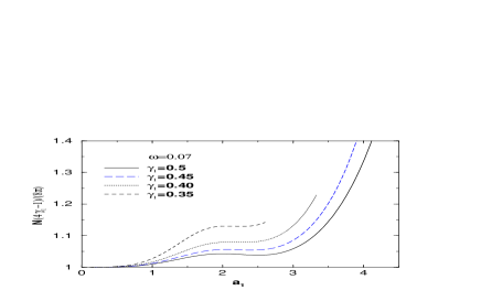
Figure 4: VA results for the repulsive case, with $\tilde{\gamma}_{0}=-0.1$ and $\omega$ fixed to 0.07, considering $\gamma_{1}=$ 0.35, 0.4, 0.45 and 0.5. In the upper frame we have $\mu$ versus $N/N(a_{1}=0)$; and, in the lower frame, $N/N(a_{1}=0)$ versus $a_{1}$.

Figure 5: The soliton profile in the stable region predicted by the VK criterion for $\omega=0.3$, $\tilde{\gamma}_{0}=-0.1$, $\gamma_{1}=0.4$, $\mu=0.1$, $N\approx 33$ at the time $t=50$. Solid line is x-direction, dashed line is y-direction.

In order to further check the role of the optical lattice, for the repulsive case we also investigate the case with constant $\omega$ and different values of $\gamma_{1}$. From the results shown in Fig. 3, for $\gamma_{1}=0.4$, we found appropriate to consider $\omega=0.07$, which has a marginal stability near $\mu\approx 0.05$. The results are shown in Fig. 4, where we first observe that a larger $\gamma_{1}$ can help to allow the width $a_{1}$ to increase, within the limiting condition (33). However, the marginal stability remains for corresponding different values of the chemical potential. In order to keep the plots of Fig.4 for different values of $\gamma_{1}$ in the same frames, we have normalize the number $N$ such that it is equal to one when $a_{1}$ is zero.

The plots of the evolution of profiles are presented for $\omega=$ 0 and 0.3 in Fig. 5, confirming the VK prediction. The results using the VA have good agreement with PDE prediction, as shown for $\omega=$0 and 0.3. The profile at $t=50$ is practically undistinguishable from the initial soliton form.

IV Evolution of 2D soliton under 1D periodic nonlinearity and dissipation

In this section, we will consider the case we have $\gamma_{2}\neq 0$ in (12). To study the dynamics of a 2D soliton with 1D periodic nonlinearity and dissipation, we also apply a variational approach and full numerical calculations. In the Gaussian ansatz (18) we should also include parameters related to dissipative effects and initial conditions. For a bright soliton, the ansatz can be taken in the following form:

$$u = A\exp\left[-\frac{(x-x_{0})^{2}}{2a_{1}^{2}}-\frac{y^{2}}{2a_{2}^{2}}\right]\times$$ (52)

$$\times \exp\left[{\rm i}b_{1}(x-x_{0})^{2}+{\rm i}b_{2}y^{2}+{\rm i}\phi(\tau)\right],$$

where $b_{i}$ ($i=$1,2) are related to dissipative effects, with $x_{0}$ and the phase $\phi$ related to initial condition.

The Lagrangian density for Eq.(12) is

$${\cal L}(x,\tau)=\frac{\rm i}{2}(u_{\tau}u^{\ast}-u_{\tau}^{\ast}u)-|u_{x}|^{2}-|u_{y}|^{2}+\frac{\gamma(x)}{2}|u|^{4},$$ (53)

where $\gamma(x)$ is given by (13). Next, from the ansatz (52), we obtain the corresponding averaged Lagrangian:

$$L = \int_{-\infty}^{\infty}dx\int_{-\infty}^{\infty}dy{\cal L}$$ (54)

$$= -\frac{\pi}{2}A^{2}a_{1}a_{2}\left[a_{1}^{2}(b_{1\tau}+4b_{1}^{2})+\frac{1}{a_{1}^{2}}+a_{2}^{2}(b_{2\tau}+4b_{2}^{2})\right.$$

$$+ \left.\frac{1}{a_{2}^{2}}+2\phi_{\tau}-\frac{A^{2}}{2}\left(\tilde{\gamma}_{0}+\gamma_{1}\cos(\kappa x_{0})e^{-\kappa^{2}a_{1}^{2}/8}\right)\right].$$

The equations for the soliton parameters $\eta_{i}=[A,a,b,\phi]$ in the VA are derived from(see for exampleFAGT )

$$\frac{\partial L}{\partial\eta_{i}}-\frac{d}{d\tau}\frac{\partial L}{\partial\eta_{i,\tau}}=\int_{-\infty}^{\infty}dx\int_{-\infty}^{\infty}dy[R\frac{\partial u^{\ast}}{\partial\eta_{i}}+c.c],$$ (55)

where the perturbation term $R$ is

$$R=-{\rm i}\gamma_{2}(1+\cos(\kappa x))|u|^{2}u+{\rm i}\alpha_{f}u.$$ (56)

Here we are taking into account a linear amplification term ($\alpha_{f}$) describing the atoms feeding. Finally, from the above, we obtain the following system of five coupled ordinary differential equations (ODE) to be solved for the parameters of our variational approach (VA):

$$(A^{2}a_{1}a_{2})_{\tau} = -\gamma_{2}A^{4}a_{1}a_{2}e^{-\kappa^{2}a^{2}/8}\cos(\kappa x_{0})-\gamma_{2}A^{4}a_{1}a_{2}+2\alpha_{f}A^{2}a_{1}a_{2},$$ (57)

$$(A^{2}a_{1}^{3}a_{2})_{\tau} = 8A^{2}a_{1}^{3}a_{2}b_{1}-\frac{\gamma_{2}}{2}A^{4}a_{1}^{3}a_{2}[1+\frac{1}{4}\cos(\kappa x_{0})(4-\kappa^{2}a_{1}^{2})e^{-\kappa^{2}a_{1}^{2}/8}]+2\alpha_{f}A^{2}a_{1}^{3}a_{2},$$ (58)

$$(A^{2}a_{1}a_{2}^{3})_{\tau} = 8A^{2}a_{1}a_{2}^{3}b_{2}-\frac{\gamma_{2}}{2}A^{4}a_{2}^{3}a_{1}[1+e^{-\kappa^{2}a_{1}^{2}/8}\cos(\kappa x_{0})]+2\alpha_{f}A^{2}a_{1}a_{2}^{3},$$ (59)

$$b_{1\tau} = \frac{1}{a_{1}^{4}}-4b_{1}^{2}-\frac{\tilde{\gamma}_{0}A^{2}}{4a_{1}^{2}}-\frac{\gamma_{1}A^{2}}{4a_{1}^{2}}\cos(\kappa x_{0})e^{-\kappa^{2}a_{1}^{2}/8}(1+\frac{\kappa^{2}a_{1}^{2}}{4}),$$ (60)

$$b_{2\tau} = \frac{1}{a_{2}^{4}}-4b_{2}^{2}-\frac{\tilde{\gamma}_{0}A^{2}}{4a_{2}^{2}}-\frac{\gamma_{1}A^{2}}{4a_{2}^{2}}\cos(\kappa x_{0})e^{-\kappa^{2}a_{1}^{2}/8}.$$ (61)

By taking into account that the norm $N=\pi A^{2}a_{1}a_{2}$, with $i,j=$ 1,2 ($i\neq j$), we have:

$$N_{\tau} = -\frac{\gamma_{2}N^{2}}{\pi a_{1}a_{2}}\left[1+e^{-\kappa^{2}a_{1}^{2}/8}\cos(\kappa x_{0})\right]+2\alpha_{f}N,$$ (62)

$$(a_{i}^{2})_{\tau} = 8a_{i}^{2}b_{i}+\frac{\gamma_{2}Na_{i}}{2\pi a_{j}}\left[1+e^{-\kappa^{2}a_{1}^{2}/8}\cos(\kappa x_{0})\left(1+\delta_{i,1}\frac{\kappa^{2}a_{1}^{2}}{4}\right)\right]$$ (63)

$$b_{i,\tau} = \frac{1}{a_{i}^{4}}-4b_{i}^{2}-\frac{N}{4\pi a_{i}^{3}a_{j}}\left(\gamma_{0}+\gamma_{1}\left[1+e^{-\kappa^{2}a_{1}^{2}/8}\cos(\kappa x_{0})\left(1+\delta_{i,1}\frac{\kappa^{2}a_{1}^{2}}{4}\right)\right]\right)$$ (64)

In the next, we present some of our results, when considering periodic nonlinearity with dissipative effects. Considering the scaling of observables with $\kappa$, discussed for the conservative systems in section III, which can also be verified in the present case, we have the corresponding transformation $b_{i}\to b_{i}/\kappa^{2}$.

In Fig. 6, we have results for the of full numerical simulations (PDE) for the evolution of the matter wave packet under combination of the conservative and dissipative nonlinear optical lattice in the case of the attractive condensate $\gamma_{0}=1/2$. As we can see the collapse is arrested by the dissipative nonlinear optical lattice. The results are compared with the prediction of the VA approach (ODE). We observe a good agreement of the VA with full-numerical calculations.

Figure 6: Results for the amplitude as a function of $\tau$, using variational approach (VA) and full numerical calculations. The VA and the full numerical calculations have the value of $\mu$ fixed to the same value for $\tau=0$, implying in a small shift of $A(0)$, as shown by the results.

We also have investigated the role of a deviation $\delta$ of the given norm from the critical norm, in the initial wave packet: $A\to A(1+\delta)$. The results of the full numerical simulations are presented in Fig. 7. Increasing the deviation $\delta$ from the critical norm, multiple peaks are observed, corresponding to revivals of the wave packet during the collapse. The number of peaks growths as $\delta$ varies from 0.02 to 0.5. The focusing-defocusing cycles connect the action of the periodically varying in the space with the inelastic three-body interactions. In linear conservative optical lattice, with inelastic three-body interactions, the focusing-defocusing oscillations have been studied in Ref. AS1 .

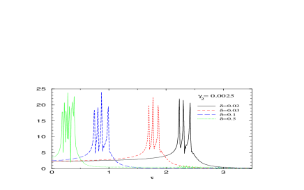
Figure 7: Results for the amplitude as a function of $\tau$, showing the collapsing behavior for $\kappa=4\pi$. The dissipation is fixed to $\gamma_{2}=0.0025$ and $\delta$ is increasing from 0.02 to 0.5.

The spreading out of the pulse after the collapse is arrested, observed in Fig. 6, can be compensated, as we note previously, by an adiabatic variation of the background scattering length, described by a time variation of $\gamma_{0}$. When we consider a time dependent $\gamma_{0}$, as given in Eq. (11), the feeding term parameter $\alpha_{f}$ should be zero, because one can show (with a redefinition of the wave-function) that it has a similar effect. In Fig. 8, we show our full numerical results confirming the stabilization of the condensate after the collapse was arrested. The mechanism of this stabilization was given by an appropriate tunning of the parameters $\alpha$ and $\tau_{c}$ of Eq. (11).

Figure 8: Soliton stabilization via compression effect, with $\tau_{c}=5$ and $\alpha=0.018$ in Eq. (11). The other parameter are $\gamma_{2}=0.006$, $\delta=0.01$, and $\kappa=4\pi$.

V Conclusion

Dynamics and stability of matter-wave solitons in the mixture of conservative and dissipative nonlinear optical lattices are investigated, considering 2D BEC, with 1D conservative plus dissipative nonlinear optical lattices.

In the first part of this work, it was analyzed conservative systems, with nonlinear optical lattices, for attractive and repulsive condensates. It was clarified the role of the scales when calculating the observables as the chemical potential and the widths. Our conclusion is that, in a 2D system, a nonlinear periodic lattice in one direction by itself cannot give stable solutions, satisfying the VK criterium VK . Such periodic lattice in the $x-$direction cannot compensate the collapsing effect which results from the other dimension. We verify that stable solutions can be obtained by controlling the soliton with a harmonic trap in the $y-$direction. For repulsive condensates, the 2D stable soliton can exist in the geometry with 1D nonlinear optical lattices in one direction and harmonic trap in the other direction.

In the second part of the work we analyze the dynamics of the above 2D system, with periodic nonlinearity in $x-$direction and without trap in the $y-$direction, when we add non-conservative nonlinear optical lattice terms. We show that the collapse of the condensate can be arrested by a dissipative periodic nonlinearity. To study the evolution of 2D wavepacket we apply the time-dependent variational approach. To compensate the wavepacket broadening, the adiabatic time variation of scattering length is used. It is shown that the metastable dissipative soliton can exist in 2D condensate with 1D periodic nonlinearity. Analytical predictions are confirmed by the numerical simulations of full 2D GP equation.

Ackhowledgments

We thank Fundação de Amparo à Pesquisa do Estado de São Paulo for partial support. LT and AG also thank Conselho Nacional de Desenvolvimento Científico e Tecnológico for partial support.

References

• (1) F.Kh. Abdullaev, A. Gammal, A.M. Kamchatnov and L. Tomio, Int. J. Mod. Phys. B 19, 3415 (2005).
• (2) B.A. Malomed, Soliton Management in Periodic Systems (Springer, New York, 2006).
• (3) I. Gabitov, and S.K. Turitsyn, Opt. Lett. 21, 327 (1996).
• (4) N.J. Smith et al., Electr. Lett. 32, 54 (1996).
• (5) F.Kh. Abdullaev, B.B. Baizakov, and M. Salerno, Phys. Rev. E 68, 066605 (2003).
• (6) L. Bergé et al., Opt. Lett. 25, 1037 (2000).
• (7) I. Towers and B.A. Malomed, J. Opt. Soc. Am. B 19, 537 (2002).
• (8) Z.Y. Xu, Y.V. Kartashov, and L. Torner, Phys.Rev.Lett. 95, 113901 (2005).
• (9) F.Kh. Abdullaev, A.M. Kamchatnov, V.V. Konotop, and V. Brazhnyi, Phys. Rev. Lett. 90, 230402 (2003).
• (10) F.Kh. Abdullaev, J.G. Caputo, B.A. Malomed, and R.A. Kraenkel, Phys. Rev. A 67, 013605 (2003).
• (11) H. Saito and M. Ueda, Phys. Rev. Lett. 90, 040403 (2003).
• (12) G.D. Montesinos, V.M. Perez-Garcia, and P.J. Torres, Physica D 191, 193 (2004).
• (13) V. Zharntsky and D. Pelinovsky, Chaos 15, 037105 (2005).
• (14) F.Kh. Abdullaev, E.N. Tsoy, B.A. Malomed, and R.A. Kraenkel, Phys. Rev. A 68, 053606 (2003).
• (15) F.Kh. Abdullaev and J. Garnier, Phys. Rev. E 72, 035603(R) (2005).
• (16) P.G. Kevrekidis, D.E. Pelinovsky, and A. Stefanov, J. Phys. A 39, 479 (2006); M.A. Porter, P.G. Kevrekidis, B.A. Malomed, and D.J. Frantzeskakis, Physica D 229, 104 (2007).
• (17) S.K. Adhikari, Phys. Rev. A 69, 063613 (2004).
• (18) Q. Quraishi, S.T. Cundiff, B.Ilan, and M. Ablowitz, Phys. Rev. Lett., 94, 243904 (2005).
• (19) M. Centurion, M.A. Porter, P.G. Kevrekidis, and D. Psaltis, Phys. Rev. Lett. 97, 033903 (2006).
• (20) P.J. Torres, Nonlinearity 19, 2103 (2006).
• (21) A. Ciattoni, C. Rizza, E. DelRe and E. Palange, Phys. Rev. Lett. 98, 043901 (2007).
• (22) F.Kh. Abdullaev and M. Salerno, J. Phys. B 36, 2851 (2003).
• (23) F.Kh. Abdullaev, A. Gammal, and L. Tomio, J. Phys. B 37, 635 (2004).
• (24) G. Theocharis et al. Phys. Rev. A 72, 033614 (2005).
• (25) F.Kh. Abdullaev and J. Garnier, Phys. Rev. A 72, 061605(R) (2005).
• (26) H. Sakaguchi and B.A. Malomed, Phys. Rev. E 72, 046610 (2005); Phys. Rev. E 73, 026601 (2006).
• (27) J.Garnier and F.Kh. Abdullaev, Phys. Rev. A 74, 01304 (2006).
• (28) J. Belmonte-Beita, V.M. Perez-Garcia, V. Vekslerchik, and P. Torres, Phys. Rev. Lett. 98, 064102 (2007).
• (29) P.O. Fedichev, Yu. Kagan, G.V. Schlyapnikov, and J.T.M. Walraven, Phys. Rev. Lett. 77, 2913 (1996).
• (30) M. Theis, et al., Phys. Rev. Lett. 93, 123001 (2004).
• (31) G. Fibich, Y. Sivan, and M.I. Weinstein, Physica D 217, 31 (2006); Phys. Rev. Lett. 97, 193902 (2006).
• (32) Y. Bludov and V.V. Konotop, Phys. Rev. A 74, 043616 (2006).
• (33) F.Kh. Abdullaev, A.A. Abdumalikov, and R.M. Galimzyanov, Phys.Lett. A in press (2007).
• (34) G. Dong and B. Hu, Phys. Rev. A 75, 013625 (2007).
• (35) G. Fibich, SIAM J. Appl. Math. 61, 1680 (2001).
• (36) P.D. Drummond and K.V. Kheruntsyan, Phys. Rev. A 63, 013605 (2001).
• (37) M. Brtka, A. Gammal, and L. Tomio, Phys.Lett. A 359, 339 (2006).
• (38) N. G. Vakhitov and A. A. Kolokolov, Radiophys. Quantum Electron. 16, 783 (1973).
• (39) V. Filho, F.Kh. Abdullaev, A. Gammal, and L. Tomio, Phys. Rev. A 63, 053603 (2001).
• (40) F.Kh. Abdullaev and M. Salerno, Phys. Rev. A 72, 033617 (2005).