Universal spectral correlations from the ballistic sigma model

Abstract

We consider the semiclassical ballistic $\sigma$-model as an effective theory describing the quantum mechanics of classically chaotic systems. Specifically, we elaborate on close analogies to the recently developed semiclassical theory of quantum interference in chaotic systems and show how semiclassical ’diagrams’ involving near action degenerate sets of periodic orbits emerge in the field theoretical description. We further discuss how the universality phenomenon (i.e. the fact that individual chaotic systems behave according to the prescriptions of random matrix theory) can be understood from the perspective of the field theory.

I Introduction

In recent years, significant progress has been made in understanding the semiclassical basis of universality in quantum chaos. In a sequence of steps aleinerlarkin ; sieber_richter01 ; smueller1 ; smueller2 ; smueller3 ; aa+haake , the theory of action correlations and periodic orbits has advanced to a stage, where the full information stored in the spectral correlation functions of random matrix theory (RMT) has become accessible by semiclassical methods. An important element in this development has been the establishment of a cross-link between semiclassics and the so-called zero dimensional sigma model (which in turn had long been known efetov to be in one-to-one correspondence to RMT): under conditions of global hyperbolicity and for low energies (energies lower than the inverse $\hbar/t_{E}$ of the so-called Ehrenfest time, $t_{E}$), individual contributions to the semiclassical expansion of spectral correlation functions become fully universal in that they depend on combinatorics and topology of the underlying orbit correlations, but not on system specific details. Each such term has a corresponding contribution to the loop expansion of the zero dimensional sigma model around one of its saddle points. From a certain perspective, the semiclassical analysis of spectral correlations has, thus, been tantamount to a reduction of the full microscopic information stored in the Green functions of an individual chaotic system down to the core data encapsulated in the zero dimensional sigma model.

In this paper, we discuss an alternative reduction scheme, which is similar in spirit, but methodologically different. Our starting point will be the observation that the zero dimensional $\sigma$-model affords an alternative interpretation, viz. as the globally uniform mean field limit of the ballistic $\sigma$-model. The ballistic $\sigma$-model in its variant considered here is an effective field theory of chaotic systems, obtained from a microscopic parent theory bsm ; ASAA1 ; ASAA2 by projection onto the sector of fields fluctuating on length scales $\gtrsim\hbar$. We will present various arguments to the effect that this projection captures the essential physics of the problem. The resulting effective field theory is defined on shells of conserved energy in classical phase space. Its dynamics is controlled by the – equally classical – Liouville operator. Quantum mechanics enters the theory through a feature known as ’non-commutativity’. In practice, non-commutativity implies that points in phase space can be defined only up to a maximal resolution set by the Planck cell. (Notice that the typical linear extensions of Planck cells are of $\mathcal{O}(\hbar^{1/2})$, much bigger than the cutoff length of the theory.) Below we will explore the conspiracy of classical hyperbolicity and Planck cell resolution in the long time dynamics of chaotic systems.

Specifically, we will show that a perturbative expansion of the model leads to structures that are remarkably similar, if not equivalent, to those arising in periodic orbit theory: taking the first quantum correction to the spectral correlation function (the ’Sieber-Richter term’ sieber_richter01 ) as an example, we will recover information on the phase space available to individual families of periodic orbits, and the corresponding action correlations. The actual integrals describing these corrections turn out to be identical to those of periodic orbit theory. This finding suggests a quantitative identification of the Feynman diagrams of the theory with the action-correlated orbit pairs of semiclassical analysis (However, an extension of the calculation to higher orders in perturbation theory, necessary to substantiate this claim, is beyond the scope of the present paper.)

Going beyond perturbation theory, we will demonstrate that for correlation energies smaller than the inverse of the Ehrenfest time non-uniform fluctuations in phase space are effectively suppressed. The resulting theory of uniform fluctuations (viz. the zero dimensional $\sigma$-model) predicts universal behavior, in agreement with the predictions of RMT. Field theory thus provides a comparatively simple way of understanding the basis of the Bohigas-Gianonni-Schmid BGS universality hypothesis, alternative to the explicit summation over infinite hierarchies of periodic orbits aa+haake . The computational efficiency of the ’mean field plus fluctuations’ approach to universality arguably represents the most important advantage of the present formalism.

The rest of the paper is organized as follows: in section II we review the semiclassical ballistic $\sigma$-model. In sections III and IV, repsectively, we explore the field theory approach to universality, and the connections to periodic orbit theory. A number of issues relating to the derivation of the theory will be addressed in appendix A.

II Ballistic $\sigma$-model

We wish to explore correlations in the level density, $\rho(E)$, of globally hyperbolic (chaotic) quantum systems, as characterized by the two point correlation function $R_{2}(s)\equiv\Delta^{2}\langle(\rho(E+{\Delta s\over 2\pi})-\langle\rho(E+{\Delta s\over 2\pi})\rangle)(\rho(E)-\langle\rho(E)\rangle)\rangle$. Here, $\langle\dots\rangle$ denotes averaging over $E$ over an interval $[E_{0}-E_{\rm av}/2,E_{0}+E_{\rm av}/2]$, where $E_{\rm av}\ll E_{0}$. The goal is to show that for energies $\omega=s\Delta/\pi\lesssim\hbar t_{\mathrm{E}}^{-1}$ the function $R_{2}(s)$ approaches the spectral correlation functions of RMT. Here, $t_{\mathrm{E}}\equiv\lambda^{-1}\ln(c^{2}/\hbar)$ is the Ehrenfest time, $\lambda$ the dominant Lyapunov exponent of the system and $c^{2}$ some classical reference scale of dimension ’action’ whose specific value will not be of much relevance. fn1

We represent the spectral correlation function in terms of a replica generating functional (Choosing the replica variant of the theory is motivated by its high suitability to perturbative calculations smueller2 ; it is a matter of a straightforward redefinition of the field target space to upgrade the formalism to a supersymmetric field theory.),

$$R_{2}(s)=-{1\over 2}{\rm Re}\,\lim_{R\to 0}{1\over R^{2}}\partial_{s}^{2}Z(s),$$ (1)

where $R$ is the number of replicas and the generating function is defined as

$$Z(s)\equiv\int DT\,\exp(-S[T]),\qquad S[T]={\beta\pi\hbar\over 2\Delta}\int_{\Gamma}(d{\bf x}){\rm tr}\Big{(}T^{-1}\ast\Lambda\{H,T\}+{is\Delta\over 2\pi\hbar}\,\Lambda T^{-1}\ast\Lambda T\Big{)}.$$ (2)

Eq. (2) has the status of an effective field theory in classical phase space, obtained from a microscopic parent theory – the energy averaged field integral representations of the microscopic Green functions bsm ; ASAA1 ; ASAA2 – by elimination of field configurations fluctuating on short scales $<\hbar$. In Appendix A we will argue that Eq. (2) relates to the microscopic formalism in much the same way the semiclassical Gutzwiller sum relates to the microscopic Feynman path integral.

The integration variables in (2), $T({\bf x})=\{T^{\alpha\alpha^{\prime}}({\bf x})\}$ are matrix valued fields defined on shells $\Gamma=\{{\bf x}|H({\bf x})=E_{0}\}$ of constant energy in classical phase space. Here, ${\bf x}\equiv({\bf q},{\bf p})$ where ${\bf q}$ and ${\bf p}$ are coordinates and momenta, respectively, $H({\bf x})$ is the Hamiltonian function of the system, and the integral over the energy-shell is normalized to unity, $\int_{\Gamma}(d{\bf x})=1$. For time reversal and spin rotation invariant systems (orthogonal symmetry class, $\beta=1$), the ’internal’ structure of the matrices $T^{\alpha\alpha^{\prime}}$ is described by a composite index $\alpha=(a,r,t)$, where $a=+/-$ discriminates between the advanced and retarded sector of the theory, $r=1,\dots,R$ is a replica index, and $t=1,2$ accounts for the operation of time reversal. Time reversal symmetry reflects in the relation $\sigma_{2}^{\rm tr}\ T^{T}\ \sigma_{2}^{\rm tr}=T^{-1}$, where $\sigma_{i}$ are Pauli matrices and the superscript ’tr’ indicates action in time reversal space. For time reversal non-invariant systems (unitary symmetry, $\beta=2$) no time-reversal structure exists and $\alpha=(a,r)$. In either case, the matrices $T$ carry a coset space structure in the sense that configurations $T$ and $TK$ are identified if $[K,\Lambda]=0$, where $\Lambda=\sigma_{3}^{\rm ar}$ and ’ar’ stands for action in advanced/retarded space.

The fluctuation behavior of the fields $T$ in (2) is governed by the classical Liouville operator $\{H,\;\}$ (where $\{\;,\;\}$ is the Poisson bracket.) Quantum mechanics enters the problem through the back-door, viz. by the presence of Moyal products ’$\ast$’ in (2). The Moyal product between two phase space functions $A$ and $B$ is defined as

$$(A\ast B)({\bf x})=\int{d^{f}{\bf x}_{1}\over(\pi\hbar)^{f}}{d^{f}{\bf x}_{2}\over(\pi\hbar)^{f}}\,e^{{2i\over\hbar}{\bf x}_{1}^{T}I{\bf x}_{2}}A({\bf x}+{\bf x}_{1})B({\bf x}+{\bf x}_{2}),$$ (3)

where $I\equiv\left(\begin{smallmatrix}0&\openone\cr-\openone&0\end{smallmatrix}\right)$ is the symplectic unit matrix. (For all practical purposes, the definition (3) will be more convenient than the standard representation moyal , $(A\ast B)({\bf x})=\exp({i\hbar\over 2}\partial^{T}_{{\bf x}^{\prime}}I\partial^{\vphantom{\dagger}}_{\bf x})\;A({\bf x}^{\prime})B({\bf x})\big{|}_{x=x^{\prime}}$.) The presence of the Moyal product implies that (a) all quantities appearing in the theory get effectively averaged (smoothened) over Planck cells. Relatedly, (b) the generator of classical time evolution $\{H,\;\}$ acts on distributions smooth in phase space on scales $\sim\hbar^{f}$, rather than on mathematical points. In the following sections we will explore how the interplay of hyperbolic dynamics ($\{H,\;\}$) and Planck cell smearing ($\ast$) determines the output of the theory.

III Universal limit

We wish to explore the behavior of the theory (2) for correlation energies $\omega\sim 2\pi\hbar\,t_{H}^{-1}\ll\hbar\,t_{\mathrm{E}}^{-1}$ of the order of the inverse Heisenberg time $t_{H}=2\pi\hbar\Delta^{-1}$ and much smaller than the inverse of the Ehrenfest time. For simplicity, we will consider systems with broken time reversal invariance throughout this section.

For energies $\omega\gg\Delta\Leftrightarrow s\gg 1$, the partition function $Z(s)$ may be evaluated by perturbative methods. To prepare the perturbative expansion of the action, we introduce the rational parameterization

$$T=\openone+W,\qquad W=\left(\begin{matrix}&-B^{\dagger}\cr B&\end{matrix}\right),$$ (4)

where the block structure is in advanced/retarded space and the generators $B$ are $R\times R$ complex matrices. Substitution of this representation then leads to a series $S[B,B^{\dagger}]=\sum_{n=1}^{\infty}S^{(2n)}[B,B^{\dagger}]$, where $S^{(n)}$ is of $n$th order in $B$ and $B^{\dagger}$. Specifically,

$$S^{(2)}[B,B^{\dagger}]=t_{H}\int_{\Gamma}(d{\bf x})\,{\rm tr}(B^{\dagger}{\cal L}_{\omega}B),$$ (5)

where

$${\cal L}_{\omega}=-i\omega/\hbar-\{H,\;\}$$ (6)

and the Moyal product stars have been omitted for notational simplicity. Higher order terms in the action contain traces over (Moyal) products of matrices $BB^{\dagger}\dots B^{\dagger}$. Due to the Planck-cell ’averaging’ inherent to the product (3), the Wick contraction of individual matrix elements of $B$ and $B^{\dagger}$ will generate expressions

$$P_{\omega}(\check{{\bf x}},\check{{\bf x}}^{\prime})=\int_{0}^{\infty}dt\,e^{i\omega t\hbar^{-1}}P_{t}(\check{\bf x},\check{\bf x}^{\prime})$$ (7)

where

$$P_{\omega}\equiv(-i\omega/\hbar-\{H,\;\})^{-1},\qquad P_{t}\equiv e^{t\{H,\;\}},$$ (8)

are the (retarded) Liouville propagators in the energy and time representation, respectively, ${\bf x}$ and ${\bf x}^{\prime}$ are arbitrary points in phase space and

$$f(\check{\bf x})\equiv{1\over\hbar^{f}}\int_{\hbar^{f}}d^{f}{\bf y}\,f({\bf x}+{\bf y})$$

is symbolic notation for coordinate averaging over a Planck cell. We interpret $P_{t}(\,\cdot\,,\check{\bf x}^{\prime})$ as the dynamical evolution of a smooth phase space distribution of extension $\hbar^{f}$ and centered around ${\bf x}^{\prime}$. It has been rigorously shown by methods of symbolic dynamics ruelle that for times $t<t_{\mathrm{E}}$, these distributions are centered around the classical trajectory through ${\bf x}^{\prime}$, i.e. the dynamics is approximately described by the Liouville evolution of ${\bf x}^{\prime}$. However, beyond $t\simeq t_{\mathrm{E}}$, the distribution rapidly (over time scales comparable to $t_{\rm mix}$) crosses over to a uniform distribution in phase space. These structures are summarized in the ansatz

$$P_{t}(\check{\bf x},\check{\bf x}^{\prime})\equiv\left\{\begin{array}[]{ll}\Omega\,\delta({\bf x}-{\bf x}^{\prime}(t)),&t\lesssim t_{\mathrm{E}},\cr 1,&t>t_{\mathrm{E}},\end{array}\right.$$ (9)

where $\Omega={h^{f}\over\Delta}$ is the volume of the energy-shell, and the normalization is such that for our unit-normalized phase space integral, $\int_{\Gamma}(d{\bf x})\,P_{t}(\check{\bf x},\check{\bf x}^{\prime})=1$.

For energy scales $\omega<\hbar t_{\mathrm{E}}^{-1}$ the dominant contribution to the time integral in (7) comes from large times $t_{\mathrm{E}}<t\lesssim\hbar\omega^{-1}$. One expects that in this regime phase space fluctuations will have effectively relaxed to spatial uniformity. To describe the damping of inhomogeneous modes in more explicit terms we follow a prescription formulated by Kravtsov and Mirlin kravtsovmirlin , then in the context of diffusive systems: employing the ansatz

$$T({\bf x})=T_{0}(1+W_{P}({\bf x}))$$ (10)

we isolate the inhomogeneous contents of the fields $T$. Here, $T_{0}={\rm const.}$ describes the zero mode sector and

$$W_{P}({\bf x})\equiv W({\bf x})-W_{Q}({\bf x}),\qquad W_{Q}({\bf x})\equiv\int_{\Gamma}(d{\bf x})\,W({\bf x}),$$

is a projection onto purely fluctuating field configurations: $\int(d{\bf x})\,W_{P}({\bf x})=0$. Substitution of Eq. (10) into the action and expansion to second order in $W_{P}=\left(\begin{smallmatrix}&-B_{P}^{\dagger}\\ B_{P}&\end{smallmatrix}\right)$ generates the decomposition

$$S[T_{0},W_{P}]=S_{0}[Q_{0}]+S^{(2)}[B^{\vphantom{\dagger}}_{P},B_{P}^{\dagger}]+S_{c}[T_{0},B^{\vphantom{\dagger}}_{P},B_{P}^{\dagger}],$$ (11)

where

$$S_{0}[Q_{0}]={i\omega\pi\over 2\Delta}{\,\rm tr}(Q_{0}\Lambda),\qquad Q_{0}=T_{0}\Lambda T_{0}^{-1}$$ (12)

is the zero mode action, and

$$S^{(2)}[B^{\vphantom{\dagger}}_{P},B_{P}^{\dagger}]=t_{H}\int_{\Gamma}(d{\bf x})\,{\rm tr}(B_{P}^{\dagger}{\cal L}_{0}B^{\vphantom{\dagger}}_{P}),$$ (13)

the quadratic action of the fluctuating fields governed by the generator ${\cal L}_{0}={\cal L}_{\omega=0}=\delta-\{H,\;\}$, $\delta\searrow 0$ of the time integrated dynamics. Finally,

$$S_{c}[T_{0},B^{\vphantom{\dagger}}_{P},B_{P}^{\dagger}]=-{i\omega t_{H}\over 2\hbar}\int_{\Gamma}(d{\bf x})\times$$ (14)

$$\times{\,\rm tr}\left((T_{0}^{-1}\Lambda T_{0})^{11}B^{\dagger}_{P}B_{P}^{\vphantom{\dagger}}-(T_{0}^{-1}\Lambda T_{0})^{22}B^{\vphantom{\dagger}}_{P}B_{P}^{\dagger}\right)({\bf x}),$$

where the superscripts refer to advanced-retarded space. Following Ref. kravtsovmirlin, , we expand in $S_{c}$, retaining only contributions of minimal order in $\omega$:

$$S_{0}[Q_{0}]\to S_{\rm eff}[Q_{0}]=S_{0}[Q_{0}]+$$

$$\hskip 8.5359pt+\langle S_{c}[T_{0},B^{\vphantom{\dagger}}_{P},B_{P}^{\dagger}]\rangle-{1\over 2}\langle(S_{c}[T_{0},B^{\vphantom{\dagger}}_{P},B_{P}^{\dagger}])^{2}\rangle,$$

where $\langle\dots\rangle\equiv\int D(B_{p}^{\vphantom{\dagger}},B_{P}^{\dagger})\,\exp(-S^{(2)}[B_{P}^{\vphantom{\dagger}},B_{P}^{\dagger}])\,(\dots)$. While the contraction of the $B$’s in the first contribution to the second line vanishes in the replica limit, the second term generates the effective action

$$S_{\rm eff}[Q_{0}]=S_{0}[Q_{0}]-{\omega^{2}\over 16\hbar^{2}}({\rm tr}(Q_{0}\Lambda))^{2}\times$$

$$\hskip 14.22636pt\times\int_{\Gamma}(d{\bf x})(d{\bf x}^{\prime})(P_{P})_{0}({\bf x},{\bf x}^{\prime})(P_{P})_{0}({\bf x}^{\prime},{\bf x}),$$ (15)

where, again, the subscript $P$ stands for projection onto the fluctuating sector:

$$(P_{P})_{0}({\bf x},{\bf x}^{\prime})\equiv\Big{(}1-\int_{\Gamma}{(d{\bf x})}\Big{)}\Big{(}1-\int_{\Gamma}{(d{\bf x}^{\prime})}\Big{)}P_{0}({\bf x},{\bf x}^{\prime})$$

$$\hskip 14.22636pt=\int_{0}^{\infty}dt\,\left(\delta({\bf x}-{\bf x}^{\prime}(t))-\Omega^{-1}\right),$$ (16)

and in the last line we have switched to a time representation. Notice that the Liouville propagator in Eq. (III) is evaluated on single phase space points, ${\bf x}$ and ${\bf x}^{\prime}$, rather than on Planck-cells $\check{\bf x}$ and $\check{\bf x}^{\prime}$. This is because the phase space integral of the Moyal-product of two operators collapses to the ordinary product jmueller , i.e.

$$\int_{\Gamma}(d{\bf x}){\,\rm tr} \left((T_{0}^{-1}\Lambda T_{0})^{11}B^{\dagger}_{P}\ast B_{P}^{\vphantom{\dagger}}\right)({\bf x})$$

$$= \int_{\Gamma}(d{\bf x}){\,\rm tr}\left((T_{0}^{-1}\Lambda T_{0})^{11}B^{\dagger}_{P}({\bf x})B_{P}^{\vphantom{\dagger}}({\bf x})\right).$$

Substituting the result Eq. (III) into Eq. (III), we obtain

$$S_{\rm eff}[Q_{0}]=S_{0}[Q_{0}]-{t_{\mathrm{E}}\Omega\over 16\hbar^{2}}(\omega{\rm tr}(Q_{0}\Lambda))^{2}\times$$ (17)

$$\hskip 14.22636pt\times\int_{0}^{\infty}dt\int_{\Gamma}(d{\bf x})\,\left(\delta({\bf x}-{\bf x}(t))-\Omega^{-1}\right).$$

According to Eq. (17), the correction term is given by the integrated weight of periodic orbits ${\bf x}\stackrel{{\scriptstyle t}}{{\to}}{\bf x}$ of duration $t$, minus the total phase volume. Using that gaspard

$$\lim_{T\rightarrow+\infty}\int_{0}^{T}dt\,\int_{\Gamma}(d{\bf x})\,\Omega\,\delta({\bf x}-{\bf x}(t))=T,$$

one concludes that this term cancels, i.e. to lowest order in the expansion, fluctuations of the inhomogeneous modes do not change the universal zero-mode action. At higher orders in the expansion, we are met with expressions (cf. Eq. (7))

$$(P_{P})_{\omega}(\check{\bf x},\check{\bf x}^{\prime})=$$

$$\hskip 5.69046pt=\int_{0}^{\infty}dt\,e^{i{\omega t\over\hbar}}\Big{(}1-\int_{\Gamma}{(d{\bf x})}\Big{)}\Big{(}1-\int_{\Gamma}{(d{\bf x}^{\prime})}\Big{)}P_{t}(\check{\bf x},\check{\bf x}^{\prime})\simeq$$

$$\hskip 5.69046pt\simeq\int_{0}^{t_{E}}dt\,e^{i{\omega t\over\hbar}}\Big{(}\Omega\delta({\bf x}-{\bf x}^{\prime}(t))-1),$$

where Eq. (9) was used. The important point here is the truncation of the time integral at $t_{E}$. This means that at $n$th order in the expansion in fluctuation propagators, $P_{P}$, corrections $\sim(\omega t_{E}/\hbar)^{n}$ will be generated. Our analysis above shows that terms with $n<3$ cancel, i.e. corrections to the zero mode action can arise only at $\mathcal{O}(\omega t_{E}\hbar^{-1})\sim\mathcal{O}(t_{E}/t_{H})^{3}$,

$$S_{\rm eff}[Q_{0}]=S_{0}[Q_{0}]+\mathcal{O}(\omega t_{E}/\hbar)^{n\geq 3}.$$

This observation is consistent with the periodic orbit analysis of Ref. a1 where it has been shown that the leading correction to the universal result scales as $(\omega t_{E}/\hbar)^{3}$.

Summarizing, our analysis shows that at correlation energies $\omega<\hbar/t_{\mathrm{E}}$ inhomogeneous fluctuations get effectively damped out and the field theory collapses to an integral over the zero mode. This means that RMT results (plus weak corrections in the parameter $(\omega t_{\mathrm{E}}/\hbar)^{n\geq 3}$) will be obtained for spectral correlation functions, and other observables probing the long time behavior of the system. Our ’mode damping’ approach to universality is complementary to semiclassical analysis aa+haake , where the spectral correlation functions are constructed explicitly, by summation over infinite hierarchies of periodic orbits. The connection between these approaches will be explored in the next section.

IV Perturbative equivalence to semiclassics

Having shown that the ballistic $\sigma$-model crosses over to the universal zero dimensional model at low energies, we now approach the problem from a different perspective. We will perform a straightforward perturbative expansion around the high energy saddle point $\Lambda$ to elaborate on parallels between the field theory (2) and the periodic orbit approach to spectral correlations. Focusing on the lowest order quantum corrections to the spectral form factor (the so-called Sieber-Richter term sieber_richter01 ), we will show that the two formalism are structurally similar, to an extent that the correlations of individual periodic orbits can be reproduced from the field theory formalism.

Throughout this section, we will consider time reversal invariant systems, i.e. $\beta=1$.

IV.1 Semiclassics

For the benefit of non-expert readers, we begin with a brief review of recent semiclassical results. Consider the Fourier transform of the spectral correlation function,

$$K(\tau)\equiv{1\over\pi}\int ds\,R_{2}(s)e^{-2is\tau}.$$ (18)

The RMT result for the $\beta=1$ form factor reads as

$$K(\tau)=\left\{\begin{array}[]{ll}2\tau-\tau\ln(1+2\tau),&\tau<1\cr 2-\tau\ln\left({2\tau+1\over 2\tau-1}\right),&\tau\geq 1.\end{array}\right.$$ (21)

Specifically, the short time expansion of the spectral form factor in $\tau\ll 1$ (corresponding to the expansion of the spectral correlation function in $\omega\gg\Delta$) starts as

$$K(\tau)=2\tau-2\tau^{2}+\dots.$$ (22)

In semiclassics one aims to reconstruct that expansion from the Gutzwiller double sum over periodic orbit pairs $(\alpha,\alpha^{\prime})$,

$$K(\tau)=\left\langle\sum_{\alpha\alpha^{\prime}}A_{\alpha}A^{\ast}_{\alpha^{\prime}}e^{{i\over\hbar}(S_{\alpha}-S_{\alpha^{\prime}})}\delta\left(\tau-{t_{\alpha}+t_{\alpha^{\prime}}\over 2t_{H}}\right)\right\rangle,$$ (23)

where $\langle\dots\rangle$ is an average over orbit energies (and a small interval of orbit times.) and $A_{\alpha},S_{\alpha}$, and $t_{\alpha}$ are the stability amplitude, the action, and the time of traversal of orbit $\alpha$, respectively.

The first term in (22) obtains from Berry’s diagonal approximation,

$$K^{(1)}(\tau)\equiv 2\tau,$$

i.e. an approximation that retains only identical orbits $\alpha=\alpha^{\prime}$ and mutually time reversed $\alpha=\overline{\alpha}^{\prime}$ orbits, and uses the Hannay-Ozorio de Almeida HOsum sum rule $\big{\langle}\sum_{\alpha}|A_{\alpha}|^{2}\delta(\tau-t_{\alpha}/t_{H})\big{\rangle}=\tau$ to determine the weight of the remaining orbit sum.

Figure 1: Cartoon of an orbit pair contributing to the first quantum correction to the spectral form factor.

The structure of the leading order (in $\tau$) quantum corrections to the spectral form factor was first identified by Aleiner and Larkin aleinerlarkin : two orbits differing in the presence or absence of a small angle self intersection in configuration space interfere to provide a stable contribution to the double sum (cf. Fig. 1.) For the sake of later comparison to the $\sigma$-model formalism, we briefly review the quantitative computation of this contribution sieber_richter01 in the invariant language of hyperbolic phase space coordinates sc2 for a system with $f=2$ degrees of freedom.

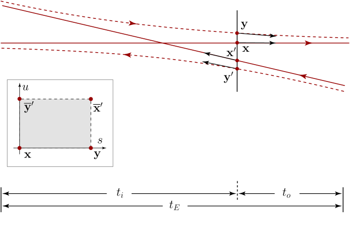
Figure 2: Phase space representation of the encounter region. Discussion, see text.

Imagine a Poincaré section cutting through the encounter region where the participating orbit segments have their (avoided) self intersection (cf. Fig. 2.) Choosing one of the piercing points, ${\bf x}$, as the origin of a local coordinate system (cf. inset of Fig. 2), we introduce $2f-1=3$ energy shell coordinates $(t,u,s)$, where $t$ is a time-like coordinate running along the trajectory through ${\bf x}$, and $u/s$ are coordinates along the locally unstable/stable directions (the existence of the latter guaranteed by the assumption of global hyperbolicity.) One may then show sieber_richter01 ; sc2 that the contribution of all orbit pairs containing a single encounter region is given by

$$K^{(2)}(\tau)=2{\tau^{2}\over h}\int duds\,e^{i\hbar^{-1}us}{t-2t_{\rm enc}(u,s)\over 2t_{\rm enc}(u,s)}=-2\tau^{2}.$$ (24)

Here, $t_{\rm enc}(u,s)=\lambda^{-1}\ln(c^{2}/us)$ is the time of traversal through the encounter region, $\lambda$ the (self-averaging) Lyapunov exponent of the system, and $c^{2}$ some classical action scale. We note that (i) the dominant contributions to the integral are of order $us\sim\hbar$ implying that $t_{\rm enc}(u,s)\sim\lambda^{-1}\ln(c^{2}/\hbar)$ is of the order of the Ehrenfest time, (ii) the product $us$ is an invariant of the motion (Liouville’s theorem), which means that the choice of the Poincaré section entering the construction is arbitrary, and (iii) the only surviving contribution to the integrand in (24) are of order ${\cal O}(t_{\rm enc}(u,s)^{0})$. (Terms containing $t_{\rm enc}$, either from the numerator, or the expansion of the denominator can be shown to effectively oscillate to zero in the semiclassical limit smueller1 ; smueller2 ; aa+haake .)

In later work, the perturbative analysis of action correlations has been extended first to cubic and then to infinite order smueller1 ; smueller2 ; smueller3 in the $\tau$-expansion. Employing an unconventional representation of the two-point correlation function aa+haake it has also been possible to reconstruct the bottom part of Eq. (21), which is not accessible in terms of a straightforward series expansion of the conventional two-Green function representation.

IV.2 Field Theory

Eq. (24) encapsulates the phase volume available to individual pairs of interfering trajectories (pre-exponent) and the corresponding action correlation (exponent). Extending the analysis of Ref. jmueller, , we will show below that the same information is stored in the effective action (2). Although our discussion will be restricted to first order in perturbation theory in $\tau$ (the extension of the analysis to higher orders in perturbation theory is left for future work), it suggests a general equivalence between periodic orbit theory and the perturbative expansion of the $\sigma$-model.

In the time reversal invariant case considered here, the blocks $B$ in (4) are $(2R\times 2R)$-matrices subject to the time reversal symmetry condition $B^{\dagger}=-\sigma_{2}^{\rm tr}\ B^{T}\sigma_{2}^{\rm tr}$.

Substitution of this representation into the action (2) generates the first order correction to the spectral correlation function

$$R_{2}(s)^{(2)}=-{\rm Re}\,\lim_{R\to 0}{t_{H}\over(2R)^{2}}\partial_{s}^{2}\int_{\Gamma}(d{\bf x})\left\langle\,{\rm tr}(B^{\dagger}BB^{\dagger}{\cal L}_{\omega}B)\right\rangle,$$

where we have omitted the Moyal product stars for the sake of notational simplicity, and averaging is over the quadratic action, $\langle\dots\rangle\equiv\int{\cal D}(B^{\dagger},B)\,e^{-S^{(2)}[B,B^{\dagger}]}(\dots)$. Doing the Gaussian integrals over matrix elements of $B$, we obtain (cf. Ref. jmueller, for technical details),

$$R^{(2)}(s)={\rm Re}\,{\Omega^{2}\over t_{H}}\partial_{s}^{2}\int_{\Gamma}(d{\bf x})\int{d{\bf y}_{1}d{\bf y}_{2}\over(2\pi\hbar)^{2(f-1)}}\,e^{{i\over\hbar}{\bf y}_{2}^{T}I{\bf y}_{1}}P_{\omega}({\bf x}+{\bf y}_{1}/2,\overline{{\bf x}-{\bf y}_{1}/2}){\cal L}_{\omega,{\bf x}+{\bf y}_{2}/2}P_{\omega}(\overline{{\bf x}+{\bf y}_{2}/2},{\bf x}-{\bf y}_{2}/2).$$

Here, $\overline{{\bf x}}\equiv({\bf q},-{\bf p})^{T}$ is the time reversed of the phase space point ${\bf x}=({\bf q},{\bf p})^{T}$, the integrals over ${\bf y}_{1}$ and ${\bf y}_{2}$ represent the generalization of the Moyal product (3) to the trace of a product of four operators and the subscript ${\bf x}$ in ${\cal L}_{\omega,{\bf x}}$ indicates on which coordinate of the propagator $P_{\omega}({\bf x},{\bf x}^{\prime})$ the derivatives of the Liouville operator act. To make further progress, we Fourier transform the expression above whereupon it transmutes to the first quantum correction to the spectral form factor,

$$K^{(2)}(\tau)=-2\tau^{2}\Omega^{2}\int_{\Gamma}(d{\bf x})\int{d{\bf y}_{1}d{\bf y}_{2}e^{\frac{i}{\hbar}{\bf y}_{2}^{T}I{\bf y}_{1}}\over(2\pi\hbar)^{2(f-1)}}\,\int_{0}^{t}dt^{\prime}P_{t-t^{\prime}}({\bf x}+{\bf y}_{1}/2,\overline{{\bf x}-{\bf y}_{1}/2}){\cal L}_{t^{\prime},{\bf x}+{\bf y}_{2}/2}P_{t^{\prime}}(\overline{{\bf x}+{\bf y}_{2}/2},{\bf x}-{\bf y}_{2}/2),$$ (25)

Here, ${\cal L}_{t}\equiv\partial_{t}-\{H,\;\}$ and $P_{t}$ is the propagator in time representation (cf. Eq. (8).) We proceed by introducing a coordinate system that has ${\bf x}$ as its origin and ${\bf x}+{\bf x}^{\prime}\leftrightarrow(r,u,s)$, where $r$ is the coordinate of ${\bf x}^{\prime}$ along the classical trajectory running through ${\bf x}$ and $u$ and $s$ parameterize the components of ${\bf x}^{\prime}$ in the locally stable and unstable direction around ${\bf x}$ (see Fig. 2.) We assume fn2 that the function $P_{t}(\overline{{\bf x}+{\bf y}/2},{\bf x}-{\bf y}/2)$ exhibits the following characteristics: (i) $P_{t}(\overline{{\bf x}+{\bf y}/2},{\bf x}-{\bf y}/2)=P_{t}(u)$ depends only on the unstable component of ${\bf y}$. Indeed, this component controls the rate at which the trajectory starting at ${\bf x}-{\bf y}/2$ deviates from that through ${\bf x}$. This deviating component (rather than the approaching component, $s$) determines the spatial and temporal structure of the Lyapunov region. Conversely, $P_{t}({\bf x}+{\bf y}/2,\overline{{\bf x}-{\bf y}/2})$ depends only on $s$. (ii) In order for $P_{t}(\overline{{\bf x}+{\bf y}/2},{\bf x}-{\bf y}/2)$ to become non-vanishing, the two trajectories through ${\bf x}-{\bf y}/2$ and $\overline{{\bf x}+{\bf y}/2}$ must have left the Lyapunov region around ${\bf x}$ (cf. the ’large scale picture’ Fig. 1). This takes a time of order $2\times t(u)$, where

$$t(u)\equiv\lambda^{-1}\ln(c/u)$$

accounts for ’half’ of the encounter time. Additional to this time, some time of classical duration, roughly of order $t_{\rm mix}$, is required to ’tie’ the outgoing and incoming trajectory segments to a closed link. These assumptions are summarized in the ansatz

$$P_{t}(\overline{{\bf x}+{\bf y}/2},{\bf x}-{\bf y}/2)=\Omega^{-1}\tilde{\Theta}(t-2t(u)),$$ (26)

where $\tilde{\Theta}$ is a smeared step function interpolating between zero and unity over a time interval of order $t_{\rm mix}$. Neither the detailed structure of $\tilde{\Theta}$, nor the exact value of $t(u)$ are of further relevance. We note, however, that the postulated independence of $P_{t}$ of the ’longitudinal’ coordinate, $r$, implies stationarity of the long time probability distribution $P_{t>t(u)}$ under the Hamiltonian flow, $\{H,P_{t>t(u)}\}=0$.

Using that ${\cal L}_{t}P_{t}\simeq\partial_{t}P_{t}$, the first quantum correction becomes ($f=2$)

$$K^{(2)}(\tau) =-{2\tau^{2}\Omega^{2}\over(2\pi\hbar)^{2}}\int_{0}^{t}dt^{\prime}\int du_{1}ds_{1}du_{2}ds_{2}\,e^{\frac{i}{\hbar}(u_{1}s_{2}-s_{1}u_{2})}P_{t-t^{\prime}}(s_{1})\partial_{t^{\prime}}P_{t^{\prime}}(u_{2})$$

$$={\tau^{2}\Omega^{2}\over 2\pi\hbar}\int_{0}^{t}dt^{\prime}\int duds\,e^{\frac{i}{\hbar}us}P_{t-t^{\prime}}(s)\partial_{t(u)}P_{t^{\prime}}(u)$$

$$\simeq{\tau^{2}\over 2\pi\hbar}\int duds\,e^{\frac{i}{\hbar}us}\partial_{t(u)}(t-2t(u)-2t(s))$$

$$={2\tau^{2}\over 2\pi\hbar}\int duds\,e^{\frac{i}{\hbar}us}\partial_{t_{\rm enc}(u,s)}{t-2t_{\rm enc}(u,s)\over 2}$$

$$={2\tau^{2}\over 2\pi\hbar}\int duds\,e^{\frac{i}{\hbar}us}{t-2t_{\rm enc}(u,s)\over 2t_{\rm enc}(u,s)},$$ (27)

in agreement with the semiclassically derived expression (24). In the first line we used that, under the conditions stated above, the long time probability distribution is invariant under the action of the Liouville operator. In the fourth line, we introduced the full encounter time, $t_{\rm enc}=t(u)+t(s)$, and the last equality is based on the above mentioned vanishing of any power $(t_{\rm enc}(u,s))^{n}$ upon integration against the oscillatory kernel $\sim\exp(i\hbar^{-1}us)$.

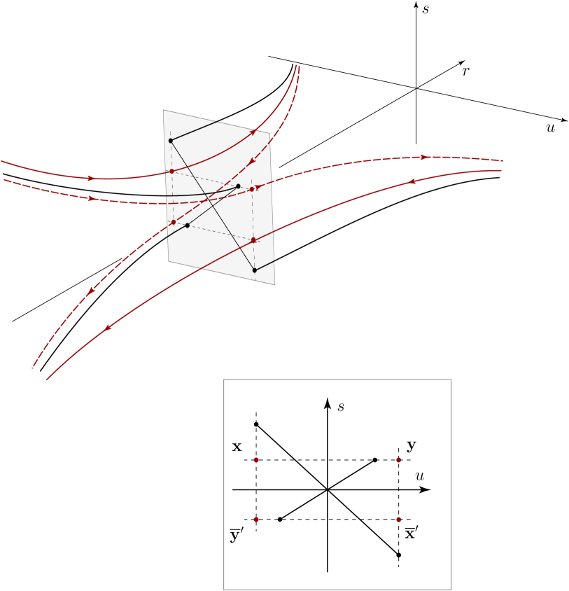
Figure 3: Assignment of propagator coordinates (lines terminating in thick points) to Feynman amplitudes (lines continued through the Poincaré section).

The derivation above demonstrates that field theory and semiclassics, resp., allocate the same phase space volume to single encounter processes. We finally show that the field theoretical expression (27) indeed affords an interpretation in terms of individual periodic orbits. To this end, we consider a Poincaré section through the encounter, as shown schematically in Fig. 3. The four lines terminating in the two pairs of connected points in the phase space plane represent segments of classical trajectories beginning at ${\bf x}+{\bf y}_{1,2}/2$ and $\overline{{\bf x}-{\bf y}_{1,2}/2}$, resp., i.e. idealized classical trajectories corresponding to the arguments of the field theory propagators in (25). Each of these points has a stable ($s$) and an unstable ($u$) coordinate. The fact that the propagators $P$ are retarded implies that we can distinguish between ’incoming’ and ’outgoing’ terminal points. Now, consider the behavior of a trajectory carrying the stable coordinate of an incoming terminal propagator point, and the unstable coordinate of a terminal point of the other propagator pair (cf. inset of Fig. 3). The trajectory running through this reference point will interpolate between the propagator stretches involved, and is naturally interpreted as part of a closed loop. The analogous definition of three more points (see inset of Fig. 3) plus associated trajectory stretches leads to the identification of a periodic orbit and its topologically distinct partner orbit. The action difference between these two orbits is but the product $us$. This construction implies an interpretation of the field theory expression (27) purely in terms of periodic orbits. The correspondence between the two formalisms is established before integration over phase space coordinates $(u,s,t)$: apparently, the action (2) encapsulates detailed information about the hyperbolic dynamics and action correlations of individual Feynman amplitudes.

V Summary and Discussion

In this paper we have considered the semiclassical ballistic $\sigma$-model as an effective theory of quantum chaos. Defined in classical phase space, the semiclassical $\sigma$-model is a field theory whose dynamics is driven by the classical Liouville operator. Quantum mechanics enters through a structure known as non-commutativity. In practice, non-commutativity (i) limits the maximal resolution of the theory to structures of the order of the Planck cell, and (ii) leads to the appearance of characteristic phases, which play a role analogous to the action correlations of periodic orbit theory.

We have shown in perturbation theory that the $\sigma$-model describes spectral correlations in far reaching analogy to semiclassics. The fact that semiclassics and field theory attribute the same weight to individual orbit correlations in phase space (cf. Eqs. (24) and (27)) makes one suspect that the $\sigma$-model fully encapsulates the information carried by the Gutzwiller double sum. However, this expectation has not been proven beyond first order in perturbation theory.

Perhaps most importantly, we have shown that the semiclassical $\sigma$-model provides for an efficient description of the crossover to the universal regime of RMT correlations at energies below the inverse of the Ehrenfest time. Adapting a technique originally developed by Kravtsov and Mirlin to describe spectral correlations in disordered systems, we saw that in chaotic systems—in contrast to disordered systems—quadratic inhomogeneous fluctuations do not give relevant corrections to the universal action. Extending this approach to higher orders in the inhomogeneous modes, a systematic quantitative estimate for the corrections to RMT spectral statistics in individual chaotic systems can, in principle, be obtained. Methodologically, this way of approaching the universality phenomenon is complementary to (and arguably more economical than) the infinite order summations over correlated orbit pairs of Refs. smueller1, ; smueller2, .

We have enjoyed fruitful discussions with P. Brouwer and F. Haake and thank S. Heusler for critical reading of the manuscript. Work supported by the Sonderforschungsbereich SFB/TR12 of the Deutsche Forschungsgemeinschaft.

Appendix A Regularization

The $\sigma$-model discussed in the foregoing sections has the status of an effective theory, obtained from an underlying ’bare’ theory by elimination of rapid fluctuations. In this section we discuss the status of that reduction. Comparing to semiclassics, we will argue that the projection onto an effective field theory resembles the passage from the Feynman path integral to the semiclassical Gutzwiller sum.

The action of the bare ballistic $\sigma$-model bsm ; ASAA1 ; ASAA2 is given by

$$S_{\rm qu}[T]=-{i\beta\pi\over 2E_{\rm av}}{\rm tr}\,\left(T^{-1}\Lambda[\hat{H},T]-{\Delta s\over 2\pi}\,\Lambda T^{-1}\Lambda T\right),$$ (28)

where, $\hat{H}$ is the Hamiltonian operator of the system and ${\rm tr}$ is a trace over Hilbert space, projected to an energy strip of with $E_{\rm av}$ centered around $E_{0}$. The integration variables $T=\{T_{{\bf q}{\bf q}^{\prime}}^{\alpha\alpha^{\prime}}\}$ are operators in a product Hilbert space spanned by real space coordinates, ${\bf q}$, and ’internal’ coordinates, $\alpha$. (The internal structure of the matrices $T_{{\bf q}{\bf q}^{\prime}}$ has been discussed in section II above.)

The action $S_{\rm qu}[T]$ is obtained from the rigorous functional integral representation of the two level correlation function after (a) a saddle point approximation (which generates the nonlinear constraint $Q^{2}=\openone$, where $Q=T\Lambda T^{-1}$) and (b) first order expansion in commutators $[\hat{H},T^{-1}]$. As we will argue in section A.2 below, these two approximations are largely immaterial.

A.1 Semiclassical Model

Preliminary contact with the (semi)classical contents of the theory is made by switching to a Wigner representation. Upon Wigner transformation of Hilbert space operators $A_{{\bf q}_{1},{\bf q}_{2}}\to A({\bf x})\equiv\int d\Delta{\bf q}\,e^{i\hbar^{-1}\Delta{\bf q}\cdot{\bf p}}A_{{\bf q}+\Delta{\bf q}/2,{\bf q}-\Delta{\bf q}/2}$, the operators $T_{{\bf q},{\bf q}^{\prime}}\to T({\bf x})$ transmute to the fields in classical phase space discussed above. fn3 Further, ${\rm tr}(\dots)\to\int_{\Gamma_{E_{\rm av}}}d^{f}{\bf x}\,(\dots)$ becomes an integral over a phase space energy shell $\Gamma_{E_{\rm av}}$, centered around $E_{0}$ and of thickness $E_{\rm av}$. We are thus led to the phase space representation jmueller

$$S_{\rm ps}[T]=-{i\beta\pi\over 2E_{\rm av}}\int_{\Gamma_{E_{\rm av}}}{d^{f}{\bf x}\over h^{f}}\,{\rm tr}\left(T^{-1}\ast\Lambda[H\stackrel{{\scriptstyle\ast}}{{,}}T]-{\omega\over 2}\,\Lambda T^{-1}\ast\Lambda T\right),$$ (29)

where the asterisks stand for Moyal products, as usual.

Importantly, the field theory (29) does not contain mechanisms inhibiting the buildup of rapid fluctuations. The action $S[T]$ of fields fluctuating on quantum scales $\sim\hbar^{\alpha}$, $\alpha\geq 1$ in classical phase space is qualitatively different from the semiclassical action considered above: for fields fluctuating transverse to the energy layer of thickness $E_{\rm av}\sim\hbar/t_{0}\sim\hbar$ reduction of the phase space integral to an integral over a single energy ’shell’ is no longer possible. Further, the series expansion of the Moyal product

$$[H\stackrel{{\scriptstyle\ast}}{{,}}T]=i\hbar\{H,T\}+\hbar^{3}\,{\cal O}(\partial^{3}H\partial^{3}T).$$

shows that for fields fluctuating on scales $\sim\hbar^{\alpha}$, $\alpha\geq 1$, the approximation of the quantum commutator by the Poisson bracket is no longer permissible.

A save way to eliminate those rapid field fluctuations is by adding a weak random potential to the Hamiltonian. An ensemble average over that randomness will generate a second order differential operator which may be tailored so as to effectively remove fast field fluctuations. As discussed in Ref. dis, a ’quantum random potential’ $V_{q}\sim\hbar$, vanishing in the classical limit (and parametrically in $\hbar$ weaker weaker than the ’regulator’ suggested by Aleiner and Larkin aleinerlarkin ; aleinerlarkin2 ) suffices to remove field fluctuations on phase space scales $\sim\hbar$.

Less rigorously, one may argue that the action $S$ of rapidly fluctuating fields will lead to highly oscillatory exponents $\exp(iS)$ which likely tend to average out: a glance at Eq. (2) shows that the largest contributions to the action of the problem, set by the largest value of the correlation energy $\omega\sim\hbar/t_{\rm mix}$, scale as $\Delta^{-1}\times\hbar$. However, fields fluctuating on scales $\sim\hbar^{\alpha}$, $\alpha\geq 1$ will lead to contributions of $\Delta^{-1}\times\hbar^{n(1-\alpha)}$, where the odd index $n$ designates the order of the Moyal expansion. One may argue that in the semiclassical limit, these terms generate strong phase cancellations which render the contribution of strongly fluctuating fields effectively meaningless. (For a caveat in this argumentation, see section A.2 below.)

We note that the above phase cancellation argument resembles the logics inherent to the stationary phase derivation of the Gutzwiller trace formula from the Feynman path integral; there, too, avoidance of rapid fluctuations is the dominant principle. More specifically, Gutzwiller’s trace formula is based on a stationary phase approximation to the Feynman path integral in $S/\hbar$ (where $S$ stands for the typical value of a classical action.) This approximation effectively averages over fine structures on scales $\hbar^{\alpha},\alpha\geq 1$. Relatedly, the semiclassical analysis of spectral correlations will be oblivious to the averaging of the system Hamiltonian over ’quantum’ perturbations $V_{q}\sim\hbar$. (Not affecting the classical dynamics, such perturbations merely change the phases weighing individual periodic orbits. In the evaluation of the Gutzwiller double sum of spectral correlations, these phases cancel out. fn4 )

Summarizing, the semiclassical $\sigma$-model (2) considered in the main text obtains as a projection of the ’quantum’ $\sigma$-model (28) onto the sector of fields fluctuating on scales $>\hbar$. This projection may be effected either by averaging the system over a quantum random potential of strength $\sim\hbar$, or by alluding to the prospected irrelevance of strongly fluctuating actions in the semiclassical limit (i.e. ad hoc restriction of the functional integral to fields fluctuating on scales $>\hbar$.)

One thus reduces the microscopic theory (equivalent to the full Feynman path integral representation of Green function correlators) to an effective theory (likely equivalent to the Gutzwiller approximation of the Feynman path integral.)

A.2 Zero modes

While the above phase cancellation arguments apply to ’generic’ field configurations, there is one family of rapidly fluctuating configurations that deserves separate consideration: the quantum action (28) is nullified by a large number of zero modes zirn fluctuating at scales of the order of the Fermi wave length. Choosing a representation in terms of eigenfunctions, $\hat{H}|\psi_{a}\rangle=\epsilon_{a}|\psi_{a}\rangle$, wherein $T=\{T^{\alpha\alpha^{\prime}}_{a,a^{\prime}}\}$ and $[\hat{H},T]=(\epsilon_{a}-\epsilon_{a}^{\prime})\{T^{\alpha\alpha^{\prime}}_{a,a^{\prime}}\}$, we conclude that there exist $N\sim E_{\rm av}/\Delta$ zero modes $T_{\alpha\alpha^{\prime}}^{aa^{\prime}}$ whose action is controlled only by the energy contribution, $S_{\rm qu}[T_{aa}]={i\beta\pi\omega\over 4E_{\rm av}}\,{\rm tr}(\Lambda T_{aa}^{-1}\Lambda T_{aa})$. Upon Wigner transformation, the zero mode operators turn into $N$ zero mode functions of the action (29), rapidly fluctuating in classical phase space. These modes are certainly not ’unphysical’. In the case of time reversal non-invariant systems, one may indeed verify nonnem that the integration over $T_{ab}$ leads to the formally exact eigenvalue decomposition

$$R_{2}(\omega)={\Delta^{2}\over E_{\rm av}}\sum_{|E_{0}-\epsilon_{a,b}|\leq E_{\rm av}/2}\delta(\omega-(\epsilon_{a}-\epsilon_{b})).$$ (30)

What makes the rigorous derivation of Eq. (30) possible is a mathematical principle known as ’semiclassical exactness’. fn5 (Incidentally, we note that the possibility to obtain an exact representation of the spectral correlation function from the quantum ballistic $\sigma$-model shows that the approximations on which the derivation of the latter is based – saddle point approximation and first order expansion in the quantum commutator – become exact in the limit $E_{\rm av}/\Delta\to\infty$.)

In spite of its formal correctness, Eq. (30) is, of course, useless in practice (much like the evaluation of the Feynman path integral in an exact basis of eigenfunctions, formally an exact alternative to the semiclassical stationary phase approximation, would be pointless.)

The conservative way to remove the zero modes is, again, by averaging over weak randomness. Indeed, semiclassical exactness represents a very delicate structure; even miniscule changes in the action will spoil the exact cancellation of all non-Gaussian fluctuations on which Eq. (30) is based. (Although we are lacking a rigorous justification, we believe that averaging over a random potential whose inverse scattering time, or level broadening, is as weak as $\hbar\tau_{q}^{-1}\sim\Delta$ will suffice to effectively remove the zero modes.) It is, then, favorable to switch to a Wigner phase space representation, and classify fluctuations along the lines of the semiclassical analysis of section A.1. Alternatively one may avoid averaging over randomness and accept the presence of zero modes – after all the integration over these modes produces a meaningful, if useless result. Mapping the integral onto a phase space representation restricted to slowly fluctuating modes one may deliberately sacrifice the exact information stored in the zero modes in return for a semiclassically meaningful approximation scheme.

References

- (1) I. L. Aleiner and A. I. Larkin, Phys. Rev. B 54, 14423 (1996).
- (2) M. Sieber and K. Richter, Physica Scripta T90, 128 (2001); M. Sieber, J. Phys. A 35, L613 (2002).
- (3) S. Müller, S. Heusler, P. Braun, F. Haake, and A. Altland, Phys. Rev. Lett. 93, 014103 (2004).
- (4) S. Müller, S. Heusler, P. Braun, H. Haake, and A. Altland, Phys. Rev. E 72, 046207 (2005).
- (5) S. Heusler, S. Müller, P. Braun, and F. Haake, J. Phys. A 37, L31 (2004).
- (6) S. Heusler, S. Müller, A. Altland, P. Braun, and F. Haake, Phys. Rev. Lett. 98, 044103 (2007).
- (7) K. B. Efetov, Adv. Phys. 32, 53 (1983).
- (8) B. A. Muzykantskii and D. E. Khmel’nitskii, JETP Lett. 62, 76 (1995).
- (9) A. V. Andreev, B. D. Simons, O. Agam, and B. L. Altshuler, Phys. Rev. Lett. 76, 3947 (1996).
- (10) A. V. Andreev, B. D. Simons, O. Agam, and B. L. Altshuler, Nucl. Phys. B 482, 536 (1996).
- (11) O. Bohigas, M. J. Giannoni, and C. Schmit, Phys. Rev. Lett. 52, 1 (1984).
- (12) For definiteness, we assume that the quantum scale exceeds the time after which the system dynamics becomes mixing. In the opposite case, the time range will be governed by a regime of irreversible, typically diffusive dynamics.
- (13) J. E. Moyal, Proc. Cambridge Philos. Soc. Math. Phys. Sci 45, 99 (1949).
- (14) D. Ruelle, Am. J. Math. 98, 619 (1976).
- (15) V. E. Kravtsov and A. D. Mirlin JETP-Lett. 60, 645 (1994).
- (16) J. Müller and A. Altland, J. Phys. A: Math. Gen. 38, 3097 (2005).
- (17) P. Gaspard, Chaos, Scattering and Statistical Mechanics (Cambridge University Press, Cambridge, 1998).
- (18) P. W. Brouwer, S. Rahav, and C. Tian, Phys. Rev. E 74, 066208 (2006).
- (19) J. H. Hannay and A. M. Ozorio de Almeida, J. Phys. A 17, 3429 (1984).
- (20) D. Spehner, J. Phys. A: Math Gen. 36, 7269 (2003).
- (21) For generic (time reversal non-invariant) systems, it is known ruelle that over a time range (the ’Ehrenfest’ time corresponding to the initial distribution) propagates the initial distribution along the classical trajectory , to then rapidly cross over to a uniform distribution . We are not aware of equally rigorous results for time reversal invariant systems.
- (22) Owing to their symmetry relations, the operators are nonlinear objects which cannot be integrated, or Wigner transformed. What we mean by is the function obtained by Wigner transformation of the (linear) generator in the exponential representation .
- (23) J. P. Müller, A Field Theory Approach to Universality in Quantum Chaos, Ph.D. thesis, Universität Köln (2007).
- (24) I. L. Aleiner and A. I. Larkin, Phys. Rev. E 55, R1243 (1997).
- (25) The action-phase correction due to reads as . The (unperturbed classical) trajectories and effectively contributing to Gutzwillers double sum are classically close , implying a vanishing of the phase differences in the semiclassical limit.
- (26) M. R. Zirnbauer, in Supersymmetrie and Trace Formulae: Chaos and Disorder, ed. by I. V. Lerner, J. P. Keating, and D. E. Khmel’nitskii (Plenum Press, New York, 1999), p. 17.
- (27) S. Nonnemacher and M. Zirnbauer, J. Math. Phys. 43, 2214 (2002).
- (28) It is a well known mathematical fact that integrals over certain manifolds (manifolds possessing a symplectic structure) may be exactly evaluated by stationary phase methods. Finite dimensional applications of this principle include the Itzykson-Zuber formulae s1 , and the mean field approach to spectral correlations for certain symmetry classes andreevaltshuler . The ballistic -model projected onto an exact eigenbasis can be treated by the same methods.
- (29) C. Itzykson and J. B. Zuber, J. Math. Phys. 21, 411 (1980).
- (30) A. V. Andreev and B. L. Altshuler, Phys. Rev. Lett. 75, 902 (1995).