Nonlinear behavior of the Chinese SSEC index with a unit root: Evidence from threshold unit root tests

Abstract

We investigate the behavior of the Shanghai Stock Exchange Composite (SSEC) index for the period from 1990:12 to 2007:06 using an unconstrained two-regime threshold autoregressive (TAR) model with an unit root developed by Caner and Hansen. The method allows us to simultaneously consider non-stationarity and nonlinearity in financial time series. Our finding indicates that the Shanghai stock market exhibits nonlinear behavior with two regimes and has unit roots in both regimes. The important implications of the threshold effect in stock markets are also discussed.

, ,

1 Introduction

In the past three decades since the Third Plenary Session of the 11th Central Committee of the Communist Party of China in December 1978, China has paved a gradual transition from a centrally planned economy to a market economy and the economy has experienced unprecedented growth. During this period, one of the most important developments has been the reopening and operation of the Chinese stock market. Before the foundation of People’s Republic of China, the Shanghai Stock Exchange was the third largest worldwide (after New York and London Stock Exchanges) and had remarkable influence on other world-class financial markets [1]. After 1949, China implemented policies of a socialist planned economy and the government controlled entirely all investment channels. In 1981, the central government began to issue treasury bonds to raise capital to cover its financial deficit, which reopened China’s securities markets. The first market for government-approved securities was founded in Shanghai on November 26, 1990 and started operating on December 19 of the same year under the name of Shanghai Stock Exchange (SHSE). Shortly after, the Shenzhen Stock Exchange (SZSE) was established on December 1, 1990 and started its operations on July 3, 1991. The size of the Chinese stock market has increased remarkably [2]. There are increasing interests in the academic studies of the Chinese stock market.

It is well-known that most econometric models are constructed based on the assumption that the variables are stationary. It is thus very important to perform unit root test for stationarity. Empirical studies on the US markets find mixed results concerning the presence of a unit root in the behavior of stock indexes [3]. The situation seems alike in the Chinese stock market. Xie, Gao and Ma applied the Phillips-Perron (PP) test to the weekly data of the Shanghai Stock Exchange Composite (SSEC) index from 12/21/1990 to 03/02/2001 and found that the null hypothesis that the logarithm of the index has a unit root cannot be rejected at the significance level of $5\%$ [4]. Cheng, Wu and Zhou tested the unit root property in the daily data of SSEC from 01/02/1998 to 12/31/2001 using the augmented Dickey-Fuller (ADF) approach and reached a similar conclusion [5]. In contrast, Dai, Yang and Zhang investigated the daily data of the SSEC index from 12/19/1990 to 06/18/2004 with the ADF approach and found that the unit root null is rejected at the $5\%$ level of significance [6].

On the other hand, numerous evidence shows that there exists threshold nonlinearity in the behavior of stocks [7, 8]. It is thus helpful to distinguish non-stationarity from nonlinearity in the stock market behavior. This task can be done by adopting the threshold unit root test developed by Caner and Hansen [9]. Briefly speaking, Caner and Hansen use threshold autoregressive (TAR) model to test for a threshold effect and then perform unit root tests on both regimes if exist. Recently, Narayan applied this method to the stock prices of Australia (ASX All Ordinaries, monthly data from 1960:01 to 2003:04) and New Zealand (NZSE Capital Index, monthly data from 1967:01 to 2003:04) [10], and the US stock price index (NYSE common stocks, monthly data from 1964:06 to 2003:04) [3]. The main finding is that the stock prices in the three markets are generated by nonlinear processes and can be characterized by unit root processes.

This work attempts to add to the existing literature by testing for nonlinearity and unit root property of the Chinese stock price index SSEC, which is monthly over the period from 1990:12 to 2007:06. We find that the monthly SSEC index behaves nonlinearly with a unit root in both regimes. The paper is organized as follows. Section 2 reviews briefly the procedure of the threshold unit root test of Caner and Hansen [9]. Section 3 presents the empirical results. And Section 4 gives some conclusive remarks.

2 Econometric methodology

In this section, we describe briefly the econometric methodology of the threshold unit root tests proposed by Caner and Hansen [9]. A rigorous presentation with assumptions, theorems and proofs can be found in their seminal paper [9]. See also references [11, 12] for a tutorial example.

2.1 Model specification and calibration

Following the work of Caner and Hansen [9], we adopt a two-regime threshold autoregression (TAR) model with an order of $k$. The mathematical expression of the TAR($k$) model reads

$$\Delta{y_{t}}={\theta_{1}x_{t-1}I(Z_{t-1}<\lambda)+\theta_{2}x_{t-1}I(Z_{t-1}\geqslant\lambda)+\epsilon_{t}}$$ (1)

with

$$x_{t-1}=(y_{t-1},1,\Delta{y_{t-1}},\cdots,\Delta{y_{t-k}})^{{}^{\prime}}~{},$$ (2)

where $y$ is the logarithm of the SSEC index for $t=1,2,\cdots,T$, $\epsilon_{t}$ is an i.i.d. error, $I({\rm{expression}})$ is the indicator function that equals to 1 if the expression in the parentheses is true and 0 otherwise, $Z_{t}=y_{t}-y_{t-m}$ for some $m\geqslant 1$ is the threshold variable, and $k\geqslant 1$ is the autoregressive order. The variable $Z_{t}$ has clear financial meaning acting as return at the time horizon of $m$ months. The threshold parameter $\lambda$ is unknown and represents the level of the variable $y_{t}$ that triggers a “regime change”, if any. The components of $\theta_{1}$ and $\theta_{2}$ can be partitioned as follows:

$$\left\{\begin{array}[]{ccc}\theta_{1}&=&\left(\rho_{1},\beta_{1},\alpha_{1}\right)\\ \theta_{2}&=&\left(\rho_{2},\beta_{2},\alpha_{2}\right)\end{array}\right.,$$ (3)

where $\rho_{1}$ and $\rho_{2}$ are slope coefficients on $y_{t-1}$, $\beta_{1}$ and $\beta_{2}$ are scalar intercepts, and $\alpha_{1}$ and $\alpha_{2}$ are $1\times k$ vectors containing the slope coefficients on dynamics regressors $(\Delta y_{t-1},\ldots,\Delta y_{t-k})$ in the two regimes.

In order to calibrate model (1), the concentrated least squares approach is usually utilized. The regression procedure is carried out for each value of $m$. The value of $\lambda$ is taken from a compact interval $[\lambda_{1},\lambda_{2}]$ in which $\lambda_{1}$ and $\lambda_{2}$ are determined by the following constraints

$$\left\{\begin{array}[]{ccc}\Pr(Z_{t}\leqslant\lambda_{1})&=&\pi_{1}\\ \Pr(Z_{t}\leqslant\lambda_{2})&=&\pi_{2}\end{array}\right.,$$ (4)

where $0<\pi_{1}<\pi_{2}<1$ and $\pi_{1}+\pi_{2}=1$. In this work, we impose $\pi_{1}=0.15$ [11]. For each $\lambda\in[\lambda_{1},\lambda_{2}]$, the parameters $\rho$’s, $\beta$’s and $\alpha$’s are estimated by minimizing the objective function

$$Q(\lambda,m)=\sum_{t=1}^{T}\epsilon_{t}(\lambda,m)^{2}~{}.$$ (5)

Let $\hat{\epsilon}_{t}(\lambda,m)$ represents the residual from the ordinary least squares for given $\lambda$ and $m$. Then the least squares estimate $\hat{\lambda}$ of the threshold parameter is given by

$$\hat{\lambda}=\min_{\lambda\in[\lambda_{1},\lambda_{2}]}\hat{Q}(\lambda,m)~{}.$$ (6)

Note that $\hat{\lambda}$ and other estimates of parameters are dependent of $m$.

2.2 Test for threshold effect

In model (1), a question of particular interest is whether or not there is a threshold effect. The threshold effect disappears under the null hypothesis

$$H_{0}:\theta_{1}=\theta_{2}~{},$$ (7)

which is tested using a standard heteroskedastic-consistent Wald test [9]. The Wald statistic is

$$W=W(\hat{\lambda})=\sup_{\lambda\in[\lambda_{1},\lambda_{2}]}W(\lambda)~{}.$$ (8)

If the null hypothesis can not be rejected, there is no threshold effect, in which case the two vectors of coefficients are identical between the two regimes ($\theta_{1}=\theta_{2}$). Caner and Hansen also show that $\sup_{\lambda\in[\lambda_{1},\lambda_{2}]}W(\lambda)$ has a non-standard asymptotic null distribution and propose a bootstrap method to compute the asymptotic critical values and $p$-values [9].

2.3 Tests for threshold unit root

When there are two regimes delimited by a threshold, we have two parameters $\rho_{1}$ and $\rho_{2}$ controlling the stationarity of the process $y_{t}$. The null hypothesis is

$$H_{0}:\rho_{1}=\rho_{2}=0~{}.$$ (9)

When the null hypothesis $H_{0}$ holds, the process $y_{t}$ has a unit root and model (1) can be expressed in terms of the stationary difference $\Delta{y_{t}}$. An alternative hypothesis to the null $H_{0}$ is

$$H_{1}:\rho_{1}<0~{}~{}~{}~{}{\rm{and}}~{}~{}~{}~{}\rho_{2}<0~{}.$$ (10)

When $H_{1}$ holds, the process $y_{t}$ is stationary and ergodic in both regimes [9]. Another alternative deals with a partial unit root, which is expressed as follows

$$H_{2}:\left\{\begin{array}[]{cccc}\rho_{1}<0&{\rm{and}}&\rho_{2}=0,&{\rm{or}}\\ \rho_{1}=0&{\rm{and}}&\rho_{2}<0.&\end{array}\right.$$ (11)

When $H_{2}$ holds, the process $y_{t}$ have a unit root in one regime and is stationary in the other showing mean reversion behavior.

To test the null hypothesis $H_{0}$ against its two alternatives $H_{1}$ and $H_{2}$, there are two Wald tests that apply. The statistic of one-sided Wald test against the unrestricted alternative $\rho_{1}\neq 0$ or $\rho_{2}\neq 0$ is

$$R_{1}=t_{1}^{2}I(\hat{\rho}_{1}<0)+t_{2}^{2}I(\hat{\rho}_{2}<0)~{},$$ (12)

while that of the two-sided Wald test against $\rho_{1}<0$ or $\rho_{2}<0$ is

$$R_{2}=t_{1}^{2}+t_{2}^{2}~{},$$ (13)

where $t_{1}$ and $t_{2}$ are the $t$ ratios for $\hat{\rho}_{1}$ and $\hat{\rho}_{2}$. We note that this term $t$ should not be confused with the time $t$ in Eq. (1). In order to further discriminate the stationarity in the two regimes, we can examine the negative of the $t$ statistics $-t_{1}$ and $-t_{2}$.

3 Application to the SSEC index

3.1 The data set

We analyze the whole time series of the SSEC index. The components of the SSEC index consist of all stocks listed on the Shanghai Stock Exchange, including both A shares and B shares. It is thus an overall index reflecting the price fluctuations of the overall Shanghai stock market. The index was officially released since July 15, 1991, tracing back to December of 1990. Monthly data over the period from 1990:12 to 2007:06 are utilized for analysis. Specifically, we retrieve the closing prices of the last trading days of all months and calculate the logarithms, which give the time series $y_{t}$ defined in the preceding section.

3.2 Unit root tests

As a first step we perform conventional unit root tests of the monthly SSEC index without taking into account possible nonlinearity. The augmented Dickey-Fuller (ADF) [13], Phillips-Perron (PP) [14], and Kwiatkowski-Phillips-Schmidt-Shin (KPSS) [15] tests are adopted. We test for unit root in both the logarithm of SSEC $y_{t}$ and its first-order difference $\Delta{y_{t}}$. For the ADF and PP tests, the null hypothesis is that $y_{t}$ (resp. $\Delta{y_{t}}$) has a unit root, which utilizes the $t$-statistic. In contrast, the null of the KPSS method is the stationarity of the variable and uses the LM-statistic. The results are presented in Table 1. All tests indicate that the SSEC index is a unit root process while its first-order difference is stationary.

Table 1: Unit root tests of the monthly SSEC index without threshold effect. The augmented Dickey-Fuller (ADF), Phillips-Perron (PP) and Kwiatkowski-Phillips-Schmidt-Shin (KPSS) tests are adopted. The left panel tests for unit root in the logarithm of SSEC $y_{t}$, while the right panel tests for unit root in the first-order difference. $V_{x\%}$ is the critical value at the $x\%$ significance level.

	$\log{\rm{SSEC}}$, $y_{t}$						$\Delta\log{\rm{SSEC}}$, $\Delta{y_{t}}$
method	statistic	$V_{10\%}$	$V_{5\%}$	$V_{1\%}$	$p$-value		statistic	$V_{10\%}$	$V_{5\%}$	$V_{1\%}$	$p$-value
ADF	-0.76	-1.62	-1.94	-2.58	0.877		-2.56	-1.62	-1.94	-2.58	0.011
PP	1.55	-1.62	-1.94	-2.58	0.970		-14.6	-1.62	-1.94	-2.58	0.000
KPSS	1.28	0.35	0.46	0.73	0.000		0.16	0.35	0.46	0.73	$\gg$0.1

3.3 Threshold effect

We now use the Wald test to examine whether we can reject the linear autoregressive model in favor of a threshold model. In our model, we adopt that $k=12$. In Table 2, we report the results of the Wald test. Also listed are the bootstrap critical values at three conventional levels $10\%$, $5\%$, and $1\%$ and the bootstrap $p$-values for threshold variables of the form $Z_{t}=y_{t}-y_{t-m}$ for different delay parameters $m$ ranging from 1 to 12. The bootstrapping is carried out with 1000 and 2000 replications. The results are qualitatively the same for both cases so that we report below the results with 2000 replications. For all $m$, the null hypothesis $\theta_{1}=\theta_{2}$ of linearity is rejected at the significance level of $1\%$. In other words, the presence of a threshold effect in the monthly SSEC index is statistically significant with a $99\%$ confidence level. According to these results, the linear AR model can be rejected in favor of the TAR model.

Table 2: Wald tests for a threshold effect in the monthly SSEC index for different lags $m$. The second row gives the Walt-statistics $W$ for different $m$. The third to fifth rows show the critical Wald-statistics at three significance levels according to a bootstrap approach with 2000 replications. The last row presents the bootstrap $p$-values. The optimal delay is $\hat{m}=4$, highlighted in bold face.

$m$	1	2	3	4	5	6	7	8	9	10	11	12
$W$	84.0	100.2	120.4	127.1	88.4	63.7	68.7	102.2	113.0	102.9	87.2	110.2
$W_{10\%}$	44.1	42.7	41.8	43.0	41.8	42.0	40.1	41.5	41.2	41.1	39.3	39.9
$W_{5\%}$	54.7	50.9	51.4	52.2	53.9	52.6	51.0	50.4	51.5	51.6	48.6	51.8
$W_{1\%}$	75.5	72.6	76.5	72.5	75.6	81.1	76.7	75.5	77.2	77.2	74.8	74.7
$p$-value	$0.4\%$	$0.1\%$	$0.1\%$	${\mathbf{0.1\%}}$	$0.4\%$	$2.4\%$	$1.8\%$	$0.1\%$	$0.1\%$	$0.1\%$	$0.4\%$	$0.1\%$

The optimal value of decay $m$ can be determined exogenously, which maximizes the value of $W$ [9]. According to Table 2, the Wald statistic is maximized ($W=127.1$) when $m=4$. Hence, we take $\hat{m}=4$ as the optimal decay parameter, which results in a preferred TAR model. Accordingly, the point estimate $\hat{\lambda}$ of the threshold is determined to be $-0.1418$. For the preferred specification with $\hat{m}=4$, we report in Table 3 the least squares parameter estimates $\hat{\theta}_{1}$ and $\hat{\theta}_{2}$ with standard errors.

Table 3: Least-squares estimates of parameters from the unconstrained threshold model with an optimal decay $\hat{m}=4$. The threshold estimate is $\hat{\lambda}=-0.1418$.

		$Z_{t-1}<\hat{\lambda}$			$Z_{t-1}\geqslant\hat{\lambda}$
Regressors		Estimate	S.E.		Estimate	S.E.
$y_{t-1}$		0.0091	0.0560		-0.0109	0.0197
Intercept		-0.1272	0.4392		0.0793	0.1414
$\Delta{y_{t-1}}$		-1.9509	0.3440		0.1530	0.0705
$\Delta{y_{t-2}}$		0.0504	0.5108		-0.0495	0.0671
$\Delta{y_{t-3}}$		1.0005	0.4000		0.0978	0.0671
$\Delta{y_{t-4}}$		-0.6906	0.3871		0.0379	0.0634
$\Delta{y_{t-5}}$		0.5264	0.1916		0.0852	0.0830
$\Delta{y_{t-6}}$		-0.1085	0.1564		0.0415	0.0837
$\Delta{y_{t-7}}$		0.5258	0.1667		-0.0564	0.0983
$\Delta{y_{t-8}}$		-0.6614	0.2292		-0.0318	0.0658
$\Delta{y_{t-9}}$		1.4061	0.2966		0.2429	0.0626
$\Delta{y_{t-10}}$		1.1534	0.3654		-0.0484	0.0656
$\Delta{y_{t-11}}$		-0.5198	0.3796		0.2115	0.0634
$\Delta{y_{t-12}}$		0.8813	0.2942		-0.0290	0.0668

The TAR model identifies two regimes depending on whether the variable $Z_{t}=y_{t}-y_{t-4}$ lies above or below the threshold $\hat{\lambda}=-0.1418$. The first regime is when $Z_{t}<-0.1418$, which occurs when the SSEC index has fallen cumulatively more than $14.18\%$ in the last four months. About 16.4% of the observations fall into this first regime. The second regime is for $Z_{t}\geqslant-0.1418$, which constitutes all those observations that occur when the $m$-month price variation is no less than $-0.1418$. Approximately $83.6\%$ of the observations belong to the second regime. Figure 1 shows the estimated division of the SSEC index into two regimes.

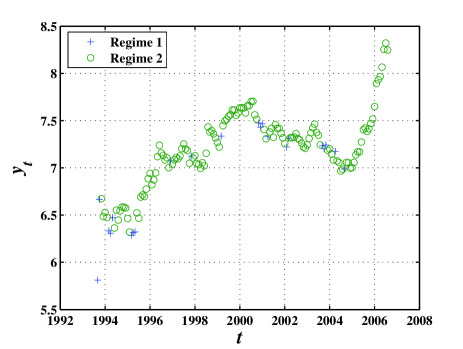
Figure 1: Monthly data of the SSEC index classified by threshold regime. The first regime (“Regime 1” in the legend) constitutes observations with the cumulative price drop greater than $14.18\%$ in the last four months.

3.4 Threshold unit root tests

We examine the unit root properties of the SSEC index that possesses significant threshold effect. We first compute the one-sided and two-sided threshold unit root test statistics $R_{1}$ and $R_{2}$ together with the bootstrap critical values at three significance levels $10\%$, $5\%$ and $1\%$ and $p$-values for each delay parameter $m$, ranging from 1 to 12. The critical Wald-statistics at three significance levels as well as the $p$-values are calculated according to a bootstrap approach with 2000 replications. The results are reported in Table 4. The one-sided Wald tests in the left panel of Table 4 show that the statistic $R_{1}$ is less than $W_{10\%}$. The situation is similar for the two-sided Wald tests presented in the right panel of Table 4. In summary, for all $m$, both $R_{1}$ and $R_{2}$ are less than the critical value at the $10\%$ level of significance. These results suggest that the null hypothesis of the presence of a unit root in the monthly SSEC index cannot be rejected at the $10\%$ level of significance.

Table 4: One-sided (left panel) and two-sided (right panel) Wald tests for threshold unit roots in the monthly SSEC index for different lags $m$. The optimal delay is $\hat{m}=4$, highlighted in bold face.

	One-sided Wald test, $R_{1}$						Two-sided Wald test, $R_{2}$
$m$	$R_{1}$	$W_{10\%}$	$W_{5\%}$	$W_{1\%}$	$p$-value		$R_{2}$	$W_{10\%}$	$W_{5\%}$	$W_{1\%}$	$p$-value
1	0.9	11.2	14.6	23.9	0.838		4.2	11.5	15.0	23.9	0.511
2	1.1	11.2	14.1	22.8	0.819		8.3	11.6	14.5	23.0	0.216
3	4.5	11.9	15.6	27.2	0.446		4.5	12.6	16.4	27.8	0.496
4	0.3	11.7	15.4	25.5	0.922		0.3	12.1	15.6	25.7	0.975
5	0.0	12.2	16.6	31.5	0.973		0.0	12.5	17.5	31.5	0.997
6	1.0	12.0	16.4	28.0	0.845		1.0	12.5	16.5	28.9	0.901
7	3.4	12.5	16.4	30.2	0.587		3.4	12.9	16.7	30.5	0.647
8	0.1	13.1	17.2	28.2	0.954		0.2	13.5	17.6	28.6	0.978
9	1.4	12.9	17.4	33.3	0.805		1.4	13.5	18.0	33.9	0.863
10	1.0	13.0	17.6	32.0	0.857		1.7	13.5	18.0	32.5	0.845
11	0.4	13.8	18.1	35.4	0.919		0.7	14.4	19.1	37.4	0.935
12	0.4	14.7	19.7	42.6	0.911		1.9	15.0	19.9	42.6	0.815

Although both tests $R_{1}$ and $R_{2}$ cannot reject the unit root hypothesis, they are not able to discriminate between the full unit root case in both regimes and the partial unit root case in one regime. We thus test the partial unit root in the monthly SSEC index by calculating the individual $t$ statistics, $t_{1}$ and $t_{2}$. The results are reported in Table 5. The critical Wald-statistics at three significance levels as well as the $p$-values are calculated according to a bootstrap approach with 2000 replications. We find that, for all $m$, both $t_{1}$ and $t_{2}$ are less than the critical value at the $10\%$ significance level. Hence, we are again unable to reject the unit root null hypothesis in both regimes of the monthly SSEC index.

Table 5: Wald tests for threshold unit roots in the two regimes of the monthly SSEC index for different lags $m$. The optimal delay is $\hat{m}=4$, highlighted in bold face.

	$t_{1}$						$t_{2}$
$m$	$t$-stat	$t_{10\%}$	$t_{5\%}$	$t_{1\%}$	$p$-value		$t$-stat	$t_{10\%}$	$t_{5\%}$	$t_{1\%}$	$p$-value
1	-1.8	2.6	3.0	4.3	0.977		0.9	2.7	3.2	4.2	0.539
2	-2.7	2.6	3.0	4.1	0.996		1.0	2.7	3.2	4.2	0.525
3	2.0	2.6	3.1	4.4	0.207		0.7	2.8	3.4	4.6	0.628
4	-0.2	2.5	3.0	4.1	0.827		0.6	2.7	3.3	4.7	0.673
5	-0.2	2.6	3.1	4.5	0.826		-0.0	2.8	3.5	5.1	0.818
6	1.0	2.6	3.2	4.2	0.522		0.3	2.9	3.5	4.9	0.737
7	1.8	2.6	3.1	4.1	0.277		0.0	2.9	3.5	5.1	0.812
8	-0.3	2.7	3.2	4.4	0.871		0.3	2.9	3.6	4.9	0.724
9	0.5	2.7	3.2	4.3	0.708		1.1	3.0	3.6	5.6	0.517
10	-0.8	2.6	3.1	4.2	0.921		1.0	3.0	3.6	5.4	0.554
11	-0.6	2.8	3.3	4.5	0.893		0.6	3.0	3.7	5.6	0.658
12	-1.2	2.8	3.4	4.6	0.952		0.7	3.1	3.8	6.1	0.653

It is noteworthy that same conclusions are reached when we use in the above statistical test the asymptotic $p$-valued tabulated by Caner and Hansen [9].

4 Concluding remarks

In summary, we have adopted the econometric approach of threshold autoregression (TAR) with a unit root developed by Caner and Hansen [9] to analyze the monthly data of the Shanghai Stock Exchange Composite index. The SSEC index is found to have a threshold effect of $\hat{\lambda}=-0.1418$ with strong evidence. In addition, both regimes with the index variation below or above the threshold have significant unit roots, so does the whole time series. Our results indicate that the Shanghai stock market exhibits nonlinear behaviors with a unit root.

An important question arises asking what we can learn further from the fact that the stock market is nonlinear with a threshold. The presence of a threshold $\hat{\lambda}=-0.1418$ means that the market behaves differently when it falls more than $14.18\%$ in four months. This threshold effect has direct connection with the concept of large drawdowns in the sense of coarse graining in time for the former and price variation for the latter, which are usually outliers [16, 17]. By scanning different time scales, one might be able to provide evidence for such a connection.

Another closely relevant issue is the definition of crashes. A consensus is still lack. A quite feasible and unambiguous definition is based on large drawdowns [18, 19]. A systematic investigation shows that more than $50\%$ of the crashes identified are endogenously triggered that have evident preceding log-periodic power-law (LPPL) patterns [20, 21]. An alternative option is to seek for large price drops within different time windows [22]. These two methods identify partially overlapping examples of crashes. It is thus interesting to explore the possibility of having a new definition of crashes by developing a multiscale TAR approach. The idea of multiscale analysis is also related to the LPPL investigation of large financial variations [23]. It is however beyond the scope of the current work.

Similar to the parity pair of drawdown and drawup, it is natural to think of the presence of a positive threshold. This needs a three-regime threshold autoregression method with two thresholds. If there do exist two thresholds (positive and negative) in the stock market behavior, one can expect that the two-regime threshold autoregression method will result in a negative threshold in some cases as in the monthly SSEC index and a positive threshold in other cases. This calls for further studies.

Acknowledgments:

We are grateful to professor B. Hansen for providing the Matlab codes. This work was partly supported by the National Natural Science Foundation of China (Grant No. 70501011), the Fok Ying Tong Education Foundation (Grant No. 101086), and the Shanghai Rising-Star Program (No. 06QA14015).

References

- [1] D.-W. Su, Chinese Stock Markets: A Research Handbook, World Scientific, Singapore, 2003.
- [2] W.-X. Zhou, D. Sornette, Antibubble and prediction of China’s stock market and real-estate, Physica A 337 (2004) 243–268.
- [3] P. K. Narayan, The behaviour of US stock prices: Evidence from a threshold autoregressive model, Math. Comput. Simul. 71 (2006) 103–108.
- [4] B.-H. Xie, R.-X. Gao, Z. Ma, Empirical tests for the efficiency of the Chinese stock markets, J. Quant. Tech. Econ. (in Chinese) 20 (5) (2002) 100–103.
- [5] X.-J. Cheng, Z.-X. Wu, H. Zhou, The weak validity test of ST portfolio in Chinese stock market, Chinese J. Manag. Sci. (in Chinese) 11 (4) (2003) 1–4.
- [6] X.-F. Dai, J. Yang, Q.-H. Zhang, Testing Chinese stock market’s weak-form efficiency: A unit root approach, Sys. Engin. (in Chinese) 23 (11) (2005) 23–28.
- [7] P. A. Shively, The nonlinear dynamics of stock prices, Q. Rev. Econ. Fin. 43 (2003) 505–517.
- [8] C. W.-S. Chen, M. K. P. So, R. H. Gerlach, Assessing and testing for threshold nonlinearity in stock returns, Aust. N. Z. J. Stat. 47 (2005) 473–488.
- [9] M. Caner, B. Hansen, Threshold autoregression with a unit root, Econometrica 69 (2001) 1555–1596.
- [10] P. K. Narayan, Are the Australian and New Zealand stock prices nonlinear with a unit root?, Appl. Econ. 37 (2005) 2161–2166.
- [11] E. Basci, M. Caner, Are real exchange rates nonlinear or nonstationary? Evidence from a new threshold unit root test, Stud. Nonlin. Dyn. Econometr. 9 (4) (2005) Article 2.
- [12] E. Basci, M. Caner, G. Yoon, Corrigendum to “Are real exchange rates nonlinear or nonstationary? Evidence from a new threshold unit root test”, Stud. Nonlin. Dyn. Econometr. 10 (2) (2006) Replication 1.
- [13] D. A. Dickey, W. A. Fuller, Likelihood ratio statistics for autoregressive time series with a unit root, Econometrica 49 (1981) 1057–1072.
- [14] P. C. B. Phillips, P. Perron, Testing for a unit root in time series regression, Biometrika 75 (1988) 335–346.
- [15] D. Kwiatkowski, P. C. B. Phillips, P. Schmidt, Y. C. Shin, Testing the null hypothesis of stationarity against the alternative of a unit root: How sure are we that economic time series have a unit root?, J. Econometrics 54 (1992) 159–178.
- [16] A. Johansen, D. Sornette, Stock market crashes are outliers, Eur. Phys. J. B 1 (1998) 141–143.
- [17] A. Johansen, D. Sornette, Large stock market price drawdowns are outliers, J. Risk 4 (2) (2001) 69–110.
- [18] D. Sornette, Why Stock Markets Crash: Critical Events in Complex Financial Systems, Princeton University Press, Princeton, 2003.
- [19] D. Sornette, Critical market crashes, Phys. Rep. 378 (2003) 1–98.
- [20] A. Johansen, D. Sornette, Endogenous versus exogenous crashes in financial markets, in: Contemporary Issues in International Finance, Nova Science Publishers, 2005, p. in press, (http://arXiv.org/abs/cond-mat/0210509).
- [21] A. Johansen, Characterization of large price variations in financial markets, Physica A 324 (2003) 157–166.
- [22] F. S. Mishkin, E. N. White, U.S. stock market crashes and their aftermath: Implications for monetary policy, NBER working paper No. W8992. Available at SSRN: http://ssrn.com/abstract=315989 (2002).
- [23] D. Sornette, W.-X. Zhou, Predictability of large future changes in major financial indices, Int. J. Forecast. 22 (2006) 153–168.