Relativistic stars with a linear equation of state:
analogy with classical isothermal spheres and black holes

We complete our previous investigations concerning the structure and the stability of “isothermal” spheres in general relativity. This concerns objects that are described by a linear equation of state, $P=q\epsilon$, so that the pressure is proportional to the energy density. In the Newtonian limit $q\rightarrow 0$, this returns the classical isothermal equation of state. We specifically consider a self-gravitating radiation ($q=1/3$), the core of neutron stars ($q=1/3$), and a gas of baryons interacting through a vector meson field ($q=1$). Inspired by recent works, we study how the thermodynamical parameters (entropy, temperature, baryon number, mass-energy, etc) scale with the size of the object and find unusual behaviours due to the non-extensivity of the system. We compare these scaling laws with the area scaling of the black hole entropy. We also determine the domain of validity of these scaling laws by calculating the critical radius (for a given central density) above which relativistic stars described by a linear equation of state become dynamically unstable. For photon stars (self-gravitating radiation), we show that the criteria of dynamical and thermodynamical stability coincide. Considering finite spheres, we find that the mass and entropy present damped oscillations as a function of the central density. We obtain an upper bound for the entropy $S$ and the mass-energy $M$ above which there is no equilibrium state. We give the critical value of the central density corresponding to the first mass peak, above which the series of equilibria becomes unstable. We also determine the deviation from the Stefan-Boltzmann law due to self-gravity and plot the corresponding caloric curve. It presents a striking spiraling behaviour like the caloric curve of isothermal spheres in Newtonian gravity. We extend our results to $d$-dimensional spheres and show that the oscillations of mass-versus-central density disappear above a critical dimension $d_{crit}(q)$. For Newtonian isothermal stars ($q\rightarrow 0$), we recover the critical dimension $d_{crit}=10$. For the stiffest stars ($q=1$), we find $d_{crit}=9$ and for a self-gravitating radiation ($q=1/d$) we find $d_{crit}=9.96404372...$ very close to $10$. Finally, we give simple analytical solutions of relativistic isothermal spheres in two-dimensional gravity. Interestingly, unbounded configurations exist for a unique mass $M_{c}=c^{2}/(8G)$.

1 Introduction

Self-gravitating systems have a very strange thermodynamics due to the attractive long-range, unshielded nature of the gravitational potential (Padmanabhan 1990, Chavanis 2006c). In particular, they can display negative specific heats, inequivalence of statistical ensembles, and phase transitions associated with gravitational collapse. Furthermore, since these systems are spatially inhomogeneous and their energy non-additive, the usual thermodynamic limit ($N\rightarrow+\infty$ with $N/V$ fixed) is clearly irrelevant and must be reconsidered. As a result, the thermodynamical parameters have unusual scalings with respect to the number of particles or system size (see Sect. 7.1 of Chavanis 2006c). For classical self-gravitating isothermal spheres, the mass scales like the size of the object $M\sim R$, which is the exact scaling of the singular isothermal sphere. As a result, the classical thermodynamic limit (CTL) for self-gravitating systems corresponds to $N\rightarrow+\infty$ in such a way that $N/V^{1/3}$ is fixed (de Vega & Sanchez 2002). It is then found that the temperature, the energy, and the entropy scale like $T\sim 1$, $E\sim N$, and $S\sim N$ (Chavanis & Rieutord 2003). When quantum effects are taken into account, the mass scales with the radius as $M\sim R^{-3}$, which is the exact mass-radius relation for nonrelativistic white dwarf stars. As a result, the quantum thermodynamic limit (QTL) for self-gravitating fermions corresponds to $N\rightarrow+\infty$ in such a way that $NV$ is fixed. It is then found that the temperature, the energy, and the entropy scale as $T\sim N^{4/3}$, $E\sim N^{7/3}$, and $S\sim N$ (Hertel & Thirring 1971, Chavanis 2002d). These exotic scalings (with respect to conventional thermodynamics) come from the long-range action of gravity, which makes the system spatially inhomogeneous and renders the energy and the entropy non additive.

On the other hand, in the context of black hole physics, Bekenstein (1973) and Hawking (1975) have shown that the entropy of a black hole scales as its area $S\sim R^{2}$ and that its temperature (measured from an observer at infinity) scales as $T\sim 1/R$. These results largely remain mysterious and are usually considered to reflect a fundamental description of spacetime at the quantum level. In order to explain the area scaling of the entropy, researchers have invoked holography (Bousso 2002), quantum gravity, string theory, entanglement entropy (Srednicki 1993), and brick-wall models (’t Hooft 1985).

In recent works, Banks et al. (2002) and Pesci (2007) considered perfect fluids in general relativity with a linear equation of state $P=q\epsilon$ and found that for the stiffest case compatible with causality ($q=1$), the entropy scales as the area $S\sim R^{2}$ and the temperature as $T\sim 1/R$. Here, these unusual scalings are a consequence of the non-extensivity of the system due to the action of gravity. As mentioned above, exotic scalings are also encountered in Newtonian gravity. However, that purely classical systems can exhibit scaling laws analogous to black holes is intriguing and deserves further investigation. The study of these systems should evidence what, in the area scaling of the black hole entropy, is the reflect of a fundamental theory of quantum gravity and what mainly stems from the non-extensive nature of the system.

In a preceding paper (Chavanis 2002b), denoted Paper I, we studied the structure and the stability of spherically symmetric relativistic stars with a linear equation of state $P=q\epsilon$. These systems are sometimes called “isothermal” (by an abuse of language) because in the Newtonian limit $q\rightarrow 0$, they reduce to classical isothermal spheres described by the Emden equation (Chandrasekhar 1972). Just as for their Newtonian counterparts, they must be enclosed within a box (of radius $R$) so as to prevent their evaporation and make their total mass finite. For a given volume, we showed the existence of a critical mass-energy $M_{c}$ above which there is no equilibrium state. In that case the system is expected to collapse and form a black hole. Furthermore, considering the series of equilibria, we showed that the mass vs central density relation $M(\epsilon_{0})$ presents a series of damped oscillations. The configurations of hydrostatic equilibrium become unstable above a certain value of the central density $\epsilon_{0,c}$ corresponding to the maximum mass (first peak). Secondary extrema in the series of equilibria correspond to new modes of instability. We also numerically observed that the baryon number vs central density $N(\epsilon_{0})$ presents extrema at the same locations as the mass $M(\epsilon_{0})$, but we were not able to explain this observation.

A first motivation of the present paper is to clarify this result. In Sects. 2.1-2.3 and in Appendix D.1, applying the general argument of Weinberg (1972) to a system described by a linear equation of state, we show that the Oppenheimer-Volkoff equation of hydrostatic equilibrium in general relativity can be obtained by extremizing the baryon number $N[\epsilon]$ at fixed mass-energy $M[\epsilon]$. From the condition $\delta N=\mu\delta M$ (where $\mu$ is a Lagrange multiplier), it becomes clear that extrema of $M(\epsilon_{0})$ in the series of equilibria correspond to extrema of $N(\epsilon_{0})$, as we observed numerically. We also argue in Sect. 2.1 and Appendix D.2 that only maxima of baryon number $N[\epsilon]$ at fixed mass $M[\epsilon]$ are dynamically stable. More precisely, the maximization of $N[\epsilon]$ at fixed $M[\epsilon]$ forms a criterion of formal nonlinear dynamical stability for a perfect fluid with respect to the Einstein equations. In Paper I, we considered the linear dynamical stability problem and showed that the system becomes unstable after the first mass peak in the series of equilibria $M(\epsilon_{0})$. In Appendix D.2 of the present paper, we show that the first mass peak also corresponds to the point at which the hydrostatic configurations cease to be maxima of the baryon number $N[\epsilon]$ (at fixed mass) and become saddle points. Therefore, the conditions of linear and nonlinear dynamical stability coincide. Similar results are obtained for barotropic spheres described by the Euler-Poisson system in Newtonian gravity (see Chavanis 2006a).

Another motivation of our paper, inspired by the works of Banks et al. (2002) and Pesci (2007), is to investigate the scaling behaviour of the thermodynamical parameters (mass-energy $M$, baryon number $N$, entropy $S$, temperature $T$, etc) with the system size $R$. In particular, for $R\rightarrow+\infty$, it is found in Sects. 2.4 and 2.5 that $M\sim R$, $N\sim S\sim R^{\frac{3q+1}{q+1}}$, and $T\sim R^{-\frac{2q}{q+1}}$. These scaling laws were implicit in our preceding paper, but they deserve to be emphasised. We complete previous studies in two respects. In Secs. 2.6 and 2.7, we use the stability criteria obtained in Paper I and Appendix D to determine the domain of validity of these scaling laws precisely. We show that, for a fixed central density $\epsilon_{0}$, the system becomes unstable above a critical radius $R_{c}$ so that the scaling laws only hold approximately close to this maximum radius. Pure scaling-law profiles, corresponding to singular spheres with infinite central energy or to regular spheres with very large radii, are dynamically unstable. Secondly, we consider general relativistic systems of astrophysical interest described by a linear equation of state for which all the parameters entering into the scaling laws (including the multiplicative factor) can be calculated explicitly. In Sect. 3, we consider a self-gravitating radiation (photon star) corresponding to $q=1/3$. This problem was first studied by Sorkin et al. (1981) in a seminal paper. For this system, we note that the entropy is proportional to the particle number ($S=\lambda N$) and the energy is proportional to the mass ($E=Mc^{2}$). Therefore, the maximization of $N$ at fixed $M$ (dynamical stability) is equivalent to the maximization of $S$ at fixed $E$ (thermodynamical stability). We immediately conclude that the conditions of dynamical and thermodynamical stability coincide. We also note that the dynamical variational problem $\delta N=\mu\delta M$ can be rewritten in the form of a thermodynamical variational problem $\delta S=T^{-1}\delta E$ where $T=c^{2}/(\lambda\mu)$ is to be interpreted as a temperature (we shall see that $T$ corresponds to the temperature at infinity $T_{0}$ given by the Tolman relation). We can therefore apply the results of Paper I to that system. For a fixed box radius, we find that there exists a maximum mass $M_{c}=0.2465...M_{P}R/L_{P}$ (where $M_{P}$ and $L_{P}$ are the Planck mass and the Planck length) and a maximum entropy $S_{c}=0.6217...k_{B}(R/L_{P})^{3/2}$ above which there is no equilibrium state. Moreover, the series of equilibria $M(\epsilon_{0})$ and $S(\epsilon_{0})$ present damped oscillations and become unstable (dynamically and thermodynamically) above a critical central density $\epsilon_{0,c}=0.439...c^{4}/(GR^{2})$ corresponding to the first mass peak. New modes of instability appear at each secondary peaks. These stability results, which have been proved analytically in Paper I and which are developed in the present paper, complete and simplify the early analysis of Sorkin et al. (1981). For a fixed central density, the photon star becomes unstable above a critical radius $R_{c}=0.663...(c^{4}/G\epsilon_{0})^{1/2}$. For large radii, the entropy scales as $S\sim R^{3/2}$. This differs from the black hole scaling, but this is consistent with the Bekenstein inequality (Bekenstein 1981). We also determine the deviation from the Stefan-Boltzmann law due to self-gravity and plot the corresponding caloric curve. In Sect. 4.1, we find similar results for a gas of completely degenerate ultra-relativistic fermions at $T=0$ modelling the core of neutron stars. In particular, the baryon number scales as $N\sim R^{3/2}$ for $R\rightarrow+\infty$. We also consider, in Sect. 4.2, a gas of baryons interacting through a vector meson field. This model, introduced by Zel’dovich (1962), is described by a linear equation of state with $q=1$. For this system the baryon number scales as the area $N\sim R^{2}$, analogously to the black hole entropy.

A last motivation of our paper is to extend our results to a space of dimension $d$. Such generalization is quite common in black hole physics and quantum gravity, where is it advocated that extra-dimensions can appear at the micro-scales, an idea stemming from the Kaluza-Klein theory. In Newtonian gravity, the influence of the dimension of space on the laws of physics has only been considered recently (Sire & Chavanis 2002, Chavanis & Sire 2004, Chavanis 2004, 2006a, 2006b, 2007a). We have shown that the structure of the system is highly dependent on the dimensionality of space and that the problem is very rich because it involves several critical dimensions. Therefore, it is natural to complete this type of investigations. In continuity with our study of classical isothermal spheres (Sire & Chavanis 2002), we show in Sect. 5 that the oscillations in the mass-central density profile disappear above a critical dimension $d_{crit}(q)$ depending on the index $q$. Above this dimension, the configurations are stable for any central density, contrary to the case $d<d_{crit}$. This implies that the pure scaling law profiles corresponding to the singular solution are now stable. For Newtonian isothermal stars ($q\rightarrow 0$) we recover the critical dimension $d_{crit}=10$ (Sire & Chavanis 2002). For the stiffest stars ($q=1$), we find $d_{crit}=9$ and for a self-gravitating radiation ($q=1/d$), we find $d_{crit}=9.96404372...$, very close to $10$. The oscillations exist for any $q\in[0,1]$ when $d<9$, and they cease to exist for any $q\in[0,1]$ when $d\geq 10$. We also note that the dimension $d=2$ is critical so that the results obtained for $d>2$ do not pass to the limit $d\rightarrow 2$. In two-dimensional gravity, we obtain in Sect. 6 analytical expressions for the density profile of relativistic isothermal spheres for any $q$. Unexpectedly, they have a finite radius for $q\neq 1$ (and the density profile decreases like a Gaussian for $q=1$) contrary to their Newtonian analogue where the density decreases as $r^{-4}$ (see, e.g., Sire & Chavanis 2002). Furthermore, they exist at a unique mass $M_{c}=c^{2}/8G$. Similarly, classical isothermal spheres in $d=2$ exist at a unique mass $M_{c}=4k_{B}T/Gm$ for a given temperature, or equivalently at a unique temperature $k_{B}T_{c}=GMm/4$ for a given mass (see, e.g., Chavanis 2007b). Because of that, we may expect that these structures are only marginally stable.

2 Relativistic stars

In this section, we complete the results obtained in Paper I concerning the structure and the stability of relativistic stars with a linear equation of state.

2.1 The equations governing equilibrium

The condition of hydrostatic equilibrium for a spherically symmetric perfect fluid in general relativity is described by the Oppenheimer-Volkoff (1939) equation

$$\left\{1-\frac{2GM(r)}{c^{2}r}\right\}\frac{dP}{dr}=-\frac{\epsilon+P}{c^{2}}\left\{\frac{GM(r)}{r^{2}}+\frac{4\pi G}{c^{2}}Pr\right\},$$

(1)

where $P(r)$ is the pressure, $\epsilon(r)$ is the energy density, and

$$M(r)=\frac{1}{c^{2}}\int_{0}^{r}\epsilon(r)4\pi r^{2}\;dr$$ (2)

is the mass-energy contained within the sphere of radius $r$. If $R$ denotes the radius of the configuration, the total mass-energy is $M=M(R)$. We also need the baryon number $N$. It is obtained by multiplying the baryon number density $n(r)$ by the proper volume element $e^{\lambda(r)/2}4\pi r^{2}dr$ and integrating over the whole configuration. This leads to an expression of the form

$$N=\int_{0}^{R}n(r)\left[1-\frac{2GM(r)}{rc^{2}}\right]^{-1/2}4\pi r^{2}\;dr.$$ (3)

If we restrict ourselves to spherically symmetric configurations and isentropic perturbations, it can be shown that the maximization problem

$${\rm Max}\quad\{N[\epsilon,n]\quad|\quad M[\epsilon]=M\quad{\rm fixed}\},$$ (4)

determines stationary solutions of the Einstein equations that are dynamically stable (Weinberg 1972). The critical points of the baryon number $N$ at fixed mass $M$ for isentropic perturbations solve the variational problem

$$\delta N-\mu\delta M=0,$$ (5)

where $\mu$ is a Lagrange multiplier enforcing the conservation of mass. This variational principle leads to the Oppenheimer-Volkoff equation (Weinberg 1972); therefore, it determines steady states of the Einstein equations. However, these first-order variations tell nothing about the stability of the system. Only maxima of $N$ at fixed mass $M$ are dynamically stable, so we must consider the sign of the second-order variations of $N$ to settle the stability of the system. In Appendix D, we consider the case of a linear equation of state $P=q\epsilon$ (see below) so that the baryon number is a functional $N[\epsilon]$ of the energy density alone. In that case, we can evaluate the second-order variations of $N$ and study the stability of the system.

The maximization problem (4) or (255) is similar to the minimization of the energy functional ${\cal W}[\rho]$ at fixed mass $M[\rho]=M$ for a self-gravitating barotropic gas in Newtonian gravity. It is known that this minimization problem provides a criterion of formal nonlinear dynamical stability for the Euler-Poisson system (see Chavanis 2006a). Similarly, we expect that the maximization problem (4) or (255) provides a criterion of formal nonlinear dynamical stability for the Einstein equations.

2.2 The equation of state

To close the system of Eqs. (1)-(2), we need to specify an equation of state relating the pressure $P$ to the energy density $\epsilon$. The first law of thermodynamics can be expressed as

$$d\left(\frac{\epsilon}{n}\right)=-Pd\left(\frac{1}{n}\right)+Td\left(\frac{s}{n}\right),$$ (6)

where $n$ is the baryon number density and $s$ the entropy density in the rest frame. We assume in the following that the term $Td(s/n)$ can be neglected. In that case, the first law of thermodynamics reduces to

$$d\epsilon=\frac{P+\epsilon}{n}dn.$$ (7)

We now assume a “gamma law” equation of state of the form

$$P=q\epsilon\quad{\rm with}\quad q=\gamma-1.$$ (8)

In that case, Eq. (7) can be integrated at once and we find the polytropic relation

$$P=Kn^{\gamma},$$ (9)

where $K$ is a constant. Combining Eqs. (8) and (9), we find that the baryon density is related to the energy density by

$$n=\left(\frac{q}{K}\right)^{1/\gamma}\epsilon^{1/\gamma}.$$ (10)

The velocity of sound is given by $(dP/d\epsilon)^{1/2}c=q^{1/2}c$ so that the principle of causality requires $q\leq 1$. In the following, we consider $0\leq q\leq 1$ (i.e. $1\leq\gamma\leq 2$).

There are two situations where the term $Td(s/n)$ can be neglected. The first situation is when $T=0$. This is the situation that prevails in the core of neutron stars where the thermal energy is much smaller than the Fermi energy so that the neutrons are completely degenerate. The second situation is when the entropy per baryon $s/n=\lambda$ is a constant. This is the case in supermassive stars where convection keeps the star stirred up and produces a uniform entropy distribution. This is also the case for a gas of self-gravitating photons where the pressure is entirely due to radiation (see Sect. 3). For a self-gravitating radiation, the Gibbs-Duhem relation

$$\epsilon=-P+Ts+\mu n,$$ (11)

simplifies itself since the chemical potential for photons vanishes ($\mu=0$). In that case, we obtain

$$\epsilon=-P+Ts.$$ (12)

Combining the foregoing relations, we find that

$$n(r)=\frac{s(r)}{\lambda}=\left(\frac{\lambda q}{1+q}\frac{T(r)}{K}\right)^{\frac{1}{\gamma-1}},$$ (13)

$$P(r)=q\epsilon(r)={K}\left(\frac{\lambda q}{1+q}\frac{T(r)}{K}\right)^{\frac{\gamma}{\gamma-1}}.$$ (14)

These relations are valid more generally for any system with $s/n=\lambda$ constant and $\mu=0$. This is the case for example in the cosmology developed by Banks & Fischler (2001) based on the holographic principle. Central to their discussion is a perfect fluid with equation of state $P=\epsilon$ and $T\propto s\propto\epsilon^{1/2}$.

2.3 The general relativistic Emden equation

Considering the equation of state (8), we introduce the dimensionless variables $\xi$, $\psi$ and $M(\xi)$ by the relations (Chandrasekhar 1972, Chavanis 2002b)

$$\epsilon=\epsilon_{0}e^{-\psi},\qquad r=\left\{\frac{c^{4}q}{4\pi G\epsilon_{0}(1+q)}\right\}^{1/2}\xi,$$ (15)

and

$$M(r)=\frac{4\pi\epsilon_{0}}{c^{2}}\left\{\frac{c^{4}q}{4\pi G\epsilon_{0}(1+q)}\right\}^{3/2}M(\xi).$$ (16)

In terms of these variables, the Oppenheimer-Volkoff equations (1)-(2) can be reduced to the following dimensionless forms

$$\left\{1-\frac{2q}{1+q}\frac{M(\xi)}{\xi}\right\}\frac{d\psi}{d\xi}=\frac{M(\xi)}{\xi^{2}}+q\xi e^{-\psi},$$ (17)

$$\frac{dM}{d\xi}=\xi^{2}e^{-\psi}.$$ (18)

In the Newtonian limit $q\rightarrow 0$, these equations reduce to the Emden equation (Chandrasekhar 1942). Therefore, Eqs. (17)-(18) represent the general relativistic equivalent of the Emden equation. It is in this sense that relativistic stars described by a linear equation of state resemble classical isothermal spheres. Just as in Newtonian gravity, there exists a singular solution

$$e^{-\psi_{s}}=\frac{Q}{\xi^{2}},\qquad{\rm where}\qquad Q=\frac{2(1+q)}{(1+q)^{2}+4q}.$$ (19)

The singular energy density profile is

$$\epsilon_{s}=\frac{qQc^{4}}{4\pi G(1+q)}r^{-2}.$$ (20)

This solution was first found by Klein (1947) and re-discovered by numerous researchers including Misner & Zapolsky (1964), Chandrasekhar (1972), etc. Considering now the regular solutions of Eqs. (17)-(18), we can always suppose that $\epsilon_{0}$ represents the energy density at the centre of the configuration. Then, Eqs. (17)-(18) must be solved with the boundary conditions $\psi(0)=\psi^{\prime}(0)=0$. The corresponding solutions must be computed numerically and some density profiles are given in Fig. 8 of Paper I for different values of $q$. It has to be noted that the asymptotic behaviour for $\xi\rightarrow+\infty$ of the regular solutions behave like the singular sphere (20).

Since the energy density decreases as $r^{-2}$ for $r\rightarrow+\infty$, relativistic stars with a linear equation of state have an infinite mass like their Newtonian analogues (see, e.g., Chavanis 2002a). This reflects the tendency of the system to evaporate. To circumvent this difficulty, we shall enclose the system within a box of radius $R$. Then, the solution of Eqs. (17)-(18) must be terminated at the normalized box radius

$$\alpha=\left\{\frac{4\pi G\epsilon_{0}(1+q)}{c^{4}q}\right\}^{1/2}R.$$ (21)

It can be noted at that point that $\alpha$ is a measure of the central density $\epsilon_{0}$ for a given box radius $R$, or a measure of the radius $R$ for a given central density $\epsilon_{0}$. The energy density contrast is a monotonic function of $\alpha$ given by

$${\cal R}\equiv\frac{\epsilon_{0}}{\epsilon(R)}=e^{\psi(\alpha)}.$$ (22)

Finally, it is convenient in the analysis to introduce the Milne variables (Chandrasekhar 1942)

$$u=\frac{\xi e^{-\psi}}{\psi^{\prime}},\qquad v=\xi\psi^{\prime}.$$ (23)

The description of the solutions of the general relativistic Emden equation in the Milne plane is given in Paper I.

2.4 Singular solution

We first give the values of the thermodynamical parameters corresponding to the singular solution of the general relativistic Emden equation. They present exact scaling laws that share some analogies with the scaling laws for the entropy and temperature of black holes. We stress from the beginning, however, that the singular solutions are unstable. The question of the stability of regular isothermal spheres is considered in Sect. 2.6.

The singular energy and pressure profiles are

$$\epsilon(r)=\frac{P(r)}{q}=\frac{qQc^{4}}{4\pi G(1+q)}r^{-2}.$$ (24)

Using the relation (10), we find that the baryon number density and the entropy profile are given by

$$n(r)=\frac{s(r)}{\lambda}=\left[\frac{q^{2}Qc^{4}}{4\pi GK(1+q)}\right]^{\frac{1}{q+1}}r^{-\frac{2}{q+1}}.$$ (25)

From Eq. (14), the temperature profile is

$$T(r)=\frac{1+q}{\lambda q}K\left[\frac{q^{2}Qc^{4}}{4\pi GK(1+q)}\right]^{\frac{q}{q+1}}r^{-\frac{2q}{q+1}}.$$ (26)

Finally, using Eqs. (106)-(107) of Paper I, we find that the functions $\nu(r)$ and $\lambda(r)$ determining the metric are given by

$$e^{-\lambda(r)}=1-pQ,\qquad e^{\nu(r)}=Ar^{\frac{4q}{q+1}},$$ (27)

where $A$ is a constant and

$$p=\frac{2q}{1+q}.$$ (28)

Comparing Eqs. (26) and (27), we check explicitly that the Tolman relation (see Appendix B) is satisfied.

Suppose now that the singular solution is terminated by a box with radius $R$. According to Eqs. (2) and (24), the total mass is

$$M=\frac{pQc^{2}}{2G}R.$$ (29)

Therefore, we find that the mass $M$ scales linearly with the radius $R$. This is the same scaling as for the singular isothermal sphere in Newtonian gravity (see, e.g., Chavanis 2002a,b). This is also the scaling entering in the Schwarzschild relation (236). On the other hand, according to Eqs. (3) and (25), the baryon number and the total entropy can be written

$$N=\frac{S}{\lambda}=\frac{1+q}{3q+1}Q^{\frac{1}{1+q}}(1-pQ)^{-1/2}$$

$$\times 4\pi\left[\frac{q^{2}c^{4}}{4\pi GK(1+q)}\right]^{1/\gamma}R^{\frac{3q+1}{q+1}}.$$ (30)

Finally, using the Tolman relation (249) and Eq. (26), the temperature measured by an observer at infinity is given by

$$T_{0}=\frac{1+q}{\lambda q}K\left[\frac{q^{2}Qc^{4}}{4\pi GK(1+q)}\right]^{\frac{q}{q+1}}(1-pQ)^{1/2}R^{-\frac{2q}{q+1}}.$$ (31)

The surface temperature $T(R)$ has the same scaling with $R$ as $T_{0}$, differing only in the factor $(1-pQ)^{1/2}$ according to the Tolman relation.

2.5 Analogy with the black hole entropy

Some interesting analogies between relativistic stars described by a linear equation of state and black hole thermodynamics have been discussed previously by Banks et al. (2002) and Pesci (2007). Let us briefly develop their arguments in connection to the present study.

When $P=\epsilon$, the velocity of sound $(dP/d\epsilon)^{1/2}c$ is equal to the velocity of light so that Eq. (8) with $q=1$ is the stiffest equation of state compatible with the principle of causality. In that case, we see from Eqs. (2.4) and (31) that the entropy scales like the area $S\sim R^{2}$ and that the temperature scales like the inverse of the radius $T\sim 1/R$. As noticed by Banks et al. (2002), this is similar to the scaling of the Bekenstein-Hawking entropy and temperature for black holes (see Appendix A). We also note from Eq. (25) that the entropy profile scales as $s(r)\sim r^{-1}$. As discussed by Pesci (2007), this shows that the total entropy is due to the contribution of the whole volume. Therefore, for relativistic stars with a linear equation of state, the area scaling of the entropy is a volume effect resulting from the inhomogeneity of the system. This differs from the result of Oppenheim (2002) who considered self-gravitating classical systems reaching the above scaling laws for entropy and temperature while approaching the Schwarzschild radius. In this limit, he showed that all entropy lies on the surface and the area scaling of the entropy is due to external layers.

More generally, for a linear equation of state of the form (8), the entropy scales as $S\sim R^{\frac{3q+1}{q+1}}$. For $0\leq q\leq 1$, the exponent is always smaller than $2$ (the area scaling law) obtained for $q=1$. This is in agreement with the Bekenstein inequality $S\leq S_{BH}=k_{B}\pi(R/L_{P})^{2}$ (where $L_{P}$ is the Planck length). Finally, we note that the energy scales like $E\sim M\sim R$ and that the temperature scales like $T\sim R^{-\frac{2q}{q+1}}$. This leads to $E\sim T^{-\frac{q+1}{2q}}$ implying negative specific heats $C=dE/dT<0$ (see Appendix A for black holes and Sect. 3.5 for the self-gravitating radiation). The mass-energy is positive but it decreases with the temperature. In Newtonian gravity, isothermal spheres also display negative specific heats but for a completely different reason (Lynden-Bell & Wood 1968). According to the Virial theorem $2K+W=0$, we have $E\equiv K+W\sim-K\sim-\frac{3}{2}Nk_{B}T$ (where $K$ is the kinetic energy and $W$ the potential energy) leading to negative specific heats $C=dE/dT=-\frac{3}{2}Nk_{B}<0$. In that case, the energy becomes more and more negative as temperature increases. Therefore, the origin of negative specific heats for classical isothermal spheres and black holes is different.

2.6 The mass-energy

We now consider regular isothermal spheres and discuss the stability of the system along the series of equilibria and the domain of validity of the scaling laws. It is shown in Paper I that the normalized mass-energy is related to the parameter $\alpha$ by the relation

$$\chi\equiv\frac{2GM}{Rc^{2}}=\frac{pv_{0}(1-qu_{0})}{1+pv_{0}},$$ (32)

where $u_{0}=u(\alpha)$ and $v_{0}=v(\alpha)$ are the values of the Milne variables at the box radius $R$. The foregoing relation can be rewritten

$$\frac{2GM}{Rc^{2}}=\chi(\alpha).$$ (33)

It defines the series of equilibria parametrized by $\alpha$ going from $0$ to $+\infty$. For a fixed box radius $R$, we can write

$$\alpha=a\epsilon_{0}^{1/2},\quad{\rm with}\quad a=\left\{\frac{4\pi G(1+q)}{c^{4}q}\right\}^{1/2}R.$$ (34)

Therefore, $\alpha=a\epsilon_{0}^{1/2}$ is a measure of the central density so that Eq. (33) determines the relation between the total mass $M$ and the central density $\epsilon_{0}$. The corresponding curve $M(\epsilon_{0})$ is plotted in Figs. 1 and 2. It presents damped oscillations around an asymptote at $M=M_{s}\equiv\chi_{s}Rc^{2}/(2G)$ corresponding to the singular solution (29). For $\alpha\rightarrow 0$, the density is almost uniform and

$$\chi(\alpha)\sim\frac{2q}{3(1+q)}\alpha^{2}.$$ (35)

For $\alpha\rightarrow+\infty$, the density profile tends to the singular sphere (20) and

$$\chi(\alpha)\rightarrow\chi_{s}=pQ.$$ (36)

The mass is maximum for a certain value of the central density corresponding to $\alpha=\alpha_{c}$ (first peak). The maximum mass is given by

$$\frac{2GM_{c}}{Rc^{2}}=\chi_{c}.$$ (37)

The values of $\alpha_{c}$, $\chi_{c}$, and $\chi_{s}$ depend on $q$. For $q=1/3$, we have $\alpha_{c}=4.7$, $\chi_{c}=0.493$, $p=1/2$, $Q=6/7$, $\chi_{s}=3/7$ and for $q=1$, we have $\alpha_{c}=4.05$, $\chi_{c}=0.544$, $p=1$, $Q=1/2$, $\chi_{s}=1/2$. There is no equilibrium state with $M>M_{c}$. For $M<M_{c}$, the stable configurations correspond to $\alpha<\alpha_{c}$, i.e. to sufficiently small central densities. The configurations with $\alpha>\alpha_{c}$ in the series of equilibria (i.e. those located after the first mass peak) are dynamically unstable. New modes of instability appear at each mass peak. These results are proved analytically in Paper I where a linear dynamical stability analysis of box-confined systems with a linear equation of state is performed. This study is completed in Appendix D where it is shown that the first mass peak is also the point at which the steady states pass from maxima of $N[\epsilon]$ (at fixed mass) to saddle points of $N[\epsilon]$ (at fixed mass). Therefore, the system loses its stability at the first mass peak in agreement with the Poincaré turning-point argument (Katz 2003, Chavanis 2006c) applied to the series of equilibria $M(\epsilon_{0})$.

Figure 1: Mass as a function of the central density for a fixed box radius. This corresponds to the curve $\chi(\alpha)$. For a system evolving at fixed volume, the system becomes unstable at the first mass peak.

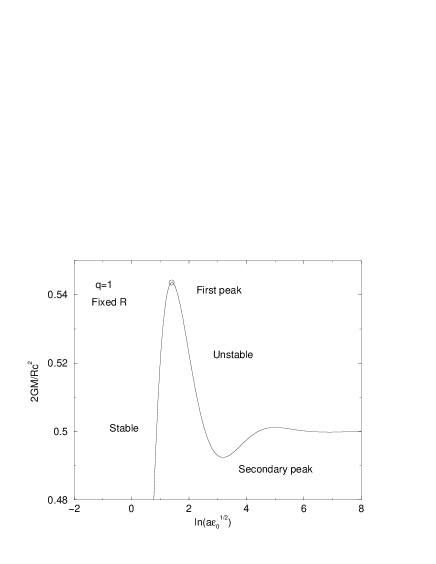
Figure 2: Mass as a function of the central density for a fixed box radius showing the secondary peaks.

For a fixed central density $\epsilon_{0}$, we can write

$$\alpha=bR,\quad{\rm with}\quad b=\left\{\frac{4\pi G\epsilon_{0}(1+q)}{c^{4}q}\right\}^{1/2}.$$ (38)

Therefore, $\alpha=bR$ is a measure of the system size $R$ so that the equation

$$M=\chi(\alpha)\frac{c^{2}R}{2G}$$ (39)

determines the relation between the total mass and the radius. In the limit $\alpha\rightarrow 0$, the system is homogeneous and, using Eq. (35), we obtain the usual scaling for an extensive system

$$M=\frac{4\pi}{3}\frac{\epsilon_{0}}{c^{2}}R^{3},\qquad(R\rightarrow 0).$$ (40)

If we now consider the limit $\alpha\rightarrow+\infty$ corresponding to the singular sphere, using Eq. (36), we get the non-extensive scaling

$$M=\chi_{s}\frac{c^{2}R}{2G},\qquad(R\rightarrow+\infty).$$ (41)

More generally, the mass-radius relation for a fixed central density is given by

$$\frac{2GbM}{c^{2}}=\chi(bR)bR.$$ (42)

This relation is plotted in Fig. 3. The scaling law $M\sim R$ is only valid in the limit $R\rightarrow+\infty$. However, as we have seen, the system becomes unstable for $R>R_{c}\equiv\alpha_{c}/b$, i.e. for a mass $M>M_{c}\equiv c^{2}R_{c}\chi_{c}/{2G}$. Therefore, the solutions exhibiting a pure scaling law profile (like the singular isothermal sphere or the regular isothermal spheres with $R\rightarrow+\infty$) are dynamically unstable. However, for stable configurations close to the critical radius $R_{c}$, we observe in Fig. 3 that the linear scaling holds approximately, so that the results given in Sect. 2.4 are correct in that sense.

Figure 3: Mass as a function of the box radius for a fixed central density. This corresponds to the curve $\alpha\chi(\alpha)$.

2.7 The baryon number

Using Eq. (3) and introducing the dimensionless variables defined previously, we find that the baryon number is given by

$$\Delta\equiv\frac{N}{N_{*}}=\frac{1}{\alpha^{\frac{3q+1}{1+q}}}\int_{0}^{\alpha}e^{-\frac{\psi(\xi)}{1+q}}\left[1-p\frac{M(\xi)}{\xi}\right]^{-1/2}\xi^{2}d\xi,$$ (43)

with

$$N_{*}=4\pi R^{3}\left[\frac{q^{2}c^{4}}{4\pi GKR^{2}(1+q)}\right]^{\frac{1}{q+1}}.$$ (44)

The foregoing relation can be rewritten

$$\frac{N}{N_{*}}=\Delta(\alpha).$$ (45)

For a fixed box radius, using $\alpha=a\epsilon_{0}^{1/2}$, this equation determines the relation between the baryon number and the central density. The corresponding curve is plotted in Fig. 4. It presents damped oscillations around an asymptote at $N=N_{s}\equiv\Delta_{s}N_{*}$ corresponding to the singular solution (2.4). According to Eq. (5) the extrema of $N(\alpha)$ occur for the same values of $\alpha$ as the extrema of $M(\alpha)$ in the series of equilibria. This leads to angular points in the curve $N(M)$, as shown in Fig. 5. For $\alpha\rightarrow 0$, corresponding to an almost uniform distribution, we have

$$\Delta(\alpha)\sim\frac{1}{3}\alpha^{\frac{2}{q+1}},$$ (46)

and for $\alpha\rightarrow+\infty$ corresponding to the singular sphere, we have

$$\Delta(\alpha)\rightarrow\Delta_{s}=\frac{1+q}{3q+1}Q^{\frac{1}{1+q}}(1-\chi_{s})^{-1/2}.$$ (47)

The baryon number is maximum for $\alpha=\alpha_{c}$ and its value is

$$\frac{N_{c}}{N_{*}}=\Delta_{c}.$$ (48)

The values of $\alpha_{c}$, $\Delta_{c}$ and $\Delta_{s}$ depend on $q$. For $q=1/3$, we have $\alpha_{c}=4.7$, $\Delta_{c}=0.925$, $\Delta_{s}=(8/21)^{1/4}=0.7856...$ and for $q=1$, we have $\alpha_{c}=4.05$, $\Delta_{c}=0.546$, $\Delta_{s}=1/2$. There is no equilibrium state with $N>N_{c}$. For $N<N_{c}$, the stable configurations correspond to $\alpha<\alpha_{c}$, i.e. to sufficiently small central densities. Configurations with $\alpha>\alpha_{c}$ in the series of equilibria are dynamically unstable. We can note that, for $q=1$, the asymptotic values $\chi_{s}=1/2$ and $\Delta_{s}=1/2$ coincide. More precisely, the curves $\chi(\alpha)$ and $\Delta(\alpha)$ turn out to superimpose for $\alpha\gg 1$. This implies that the curve $N(M)$ becomes linear in the region where $\alpha\gg 1$, as can be seen in Fig. 5. This behaviour is, however, not general and, for $q\neq 1$, the curves $\chi(\alpha)$ and $\Delta(\alpha)$ are different (see, e.g., Figs. 18 and 19 of Paper I for $q=1/3$).

Figure 4: Baryon number as a function of the central density for a fixed box radius. We have plotted $\Delta(\alpha)$.

Figure 5: Baryon number as a function of the mass for a fixed box radius. We have plotted $\Delta(\alpha)$ as a function of $\chi(\alpha)$ so that the curve is parametrized by $\alpha$. For $q=1$, we note that, asymptotically, $\Delta(\alpha)\simeq\chi(\alpha)$ so that the relation $M\sim N$ is linear. We have drawn a line $y=x$ for comparison. This special behaviour arises only for $q=1$.

For a fixed central density, using $\alpha=bR$, the equation

$$N=\Delta(\alpha)4\pi\left[\frac{q^{2}c^{4}}{4\pi GK(1+q)}\right]^{\frac{1}{q+1}}R^{\frac{3q+1}{q+1}},$$ (49)

determines the relation between the baryon number and the radius. In the limit $\alpha\rightarrow 0$, the system is homogeneous and, using Eq. (46), we have the usual scaling for an extensive system

$$N=\frac{4\pi}{3}n_{0}R^{3},\qquad(R\rightarrow 0).$$ (50)

If we now consider the limit $\alpha\rightarrow+\infty$, corresponding to the singular sphere, using Eq. (47) we find the non-extensive scaling

$$N=\Delta_{s}4\pi\left[\frac{q^{2}c^{4}}{4\pi GK(1+q)}\right]^{\frac{1}{q+1}}R^{\frac{3q+1}{q+1}},\quad(R\rightarrow+\infty).$$

(51)

More generally, for a fixed central density, the baryon number is expressed as a function of the radius by

$$\frac{1}{4\pi}\left[\frac{4\pi GK(1+q)}{q^{2}c^{4}}\right]^{\frac{1}{q+1}}b^{\frac{3q+1}{q+1}}N=(bR)^{\frac{3q+1}{q+1}}\Delta(bR).$$ (52)

This relation is plotted in Fig. 6. The scaling law $N\sim R^{\frac{3q+1}{q+1}}$ is only valid in the limit $R\rightarrow+\infty$. However, as we have seen, the system becomes unstable for $R>R_{c}\equiv\alpha_{c}/b$, i.e. for a baryon number $N>N_{c}\equiv\Delta_{c}N_{*}(R_{c})$. Therefore, the solutions exhibiting a pure scaling law profile (like the singular isothermal sphere or the regular isothermal spheres with $R\rightarrow+\infty$) are dynamically unstable. However, for the stable configurations close to the critical radius $R_{c}$, we note that the scaling $N\sim R^{\frac{3q+1}{q+1}}$ holds approximately, so that the results given in Sect. 2.4 are correct in that sense. Finally, in Fig. 7, we have plotted the curve $N(M)$ for a fixed central density. For small mass, we have the scaling $N\sim M$ and for large mass, we have $N\sim M^{\frac{3q+1}{q+1}}$.

Figure 6: Baryon number as a function of the box radius for a fixed central density. We have plotted $\alpha^{\frac{3q+1}{q+1}}\Delta(\alpha)$.

Figure 7: Baryon number as a function of the mass for a fixed central density. We have plotted $\alpha^{\frac{3q+1}{q+1}}\Delta(\alpha)$ as a function of $\alpha\chi(\alpha)$ so that the curve is parametrized by $\alpha$.

As a final remark, we note that the density contrast (22) is a monotonic function of $\alpha$ (behaving like the inverse of the density profile reported in Fig. 8 of Paper I) that could be used to parametrize the series of equilibria $M(\alpha)$ and $N(\alpha)$ in place of $\alpha$. In particular, the critical energy density contrast corresponding to $\alpha_{c}$ is ${\cal R}_{c}=30.1$ for $q=1$ and ${\cal R}_{c}=22.4$ for $q=1/3$. Configurations with a density contrast greater than these values are dynamically unstable.

3 Self-gravitating radiation: photon stars

In this section, we apply the preceding results to a radiation that is so intense that self-gravity (in the sense of general relativity) must be taken into account. This is sometimes referred to as “photon stars” (Schmidt & Homann 2000). This problem was first considered by Sorkin et al. (1981). Our work confirms and extends the results of these authors.

3.1 Equation of state for ultra-relativistic particles

Let us consider a perfect gas of non-interacting particles that can be relativistic. We call $f({\bf p})$ the numerical density of particles with impulse ${\bf p}$. The particle number, the kinetic energy, and the pressure are

$$N=V\int fd{\bf p},$$ (53)

$$E_{kin}=V\int f\epsilon(p)d{\bf p},$$ (54)

$$P=\frac{1}{3}\int fp\frac{d\epsilon}{dp}d{\bf p},$$ (55)

where the kinetic energy of a particle is

$$\epsilon(p)=mc^{2}\left\{\left(1+\frac{p^{2}}{m^{2}c^{2}}\right)^{1/2}-1\right\}.$$ (56)

In the ultra-relativistic limit, the kinetic energy of a particle with impulse $p$ reduces to

$$\epsilon(p)=pc.$$ (57)

Therefore, the pressure is related to the kinetic energy by

$$P=\frac{1}{3}\frac{E_{kin}}{V}.$$ (58)

In the local form, this leads to the linear equation of state

$$P=q\epsilon\qquad{\rm with}\quad q=\frac{1}{3}.$$ (59)

Note that, in a $d$-dimensional universe (see Sect. 5), the corresponding value of this parameter would be

$$q=\frac{1}{d}.$$ (60)

3.2 The Stefan-Boltzmann law

We first recall some basic elements of thermodynamics that apply to a pure radiation modeled as a gas of photons. We first ignore gravitational effects. The distribution function of a perfect gas of bosons without interaction is given by the Bose-Einstein statistics

$$f=\frac{1}{h^{3}}\frac{1}{e^{\beta\epsilon-\mu}-1},$$ (61)

where $\mu$ is the chemical potential. For ultra-relativistic particles, we have $\epsilon=pc$. On the other hand, for particles without rest mass, like photons, the chemical potential $\mu=0$. Therefore, the distribution function of a gas of photons is simply

$$f=\frac{1}{h^{3}}\frac{1}{e^{\beta pc}-1}.$$ (62)

The particle number, the kinetic energy, and the pressure can be computed from Eqs. (53)-(55). Writing these relations locally and using the properties of the Bose integrals, we obtain the standard results

$$P=\frac{1}{3}\epsilon=\frac{8\pi}{h^{3}c^{3}}(k_{B}T)^{4}\frac{\pi^{4}}{90},$$ (63)

$$n=\frac{8\pi}{h^{3}c^{3}}(k_{B}T)^{3}\zeta(3).$$ (64)

The relation (63) between the energy and the temperature is the Stefan-Boltzmann law. Using the Gibbs-Duhem relation (11) with $\mu=0$, we directly obtain the entropy

$$s=k_{B}\frac{32\pi^{5}}{90h^{3}c^{3}}(k_{B}T)^{3}.$$ (65)

For a pure radiation, the pressure is related to the photon density by

$$P=Kn^{\gamma},$$ (66)

with

$$\gamma=\frac{4}{3},\qquad K=\frac{\pi^{4}}{90}\frac{hc}{\left[8\pi\zeta(3)^{4}\right]^{1/3}}.$$ (67)

On the other hand, the entropy is related to the photon density by

$$s=\lambda n,\qquad{\rm with}\quad\lambda=\frac{4\pi^{4}}{90\zeta(3)}k_{B}.$$ (68)

If we now consider a gas of self-gravitating photons in general relativity (photon stars), the preceding relations still hold locally. They have the form considered in Sect. 2.2 with $q=1/3$. Therefore, a self-gravitating radiation can be studied with the theory developed in Sect. 2. We note that the singular profiles of Sect. 2.4 scale like

$$P\propto\epsilon\propto r^{-2},\qquad s\propto n\propto r^{-3/2},\qquad T\propto r^{-1/2}.$$ (69)

These are also the asymptotic behaviours of the regular profiles for $r\rightarrow+\infty$. The numerical constants in Eqs. (24)-(26) can be obtained explicitly by using the values of $K$, $\gamma$, and $\lambda$ given above.

3.3 The mass-energy of self-gravitating photons

We now apply the general results of Sect. 2.6 to the specific context of a self-gravitating radiation. The consideration of an explicit physical example allows us to determine the numerical value of the multiplicative constants appearing in the scaling laws. It is convenient to introduce the Planck length and the Planck mass,

$$L_{P}=\left(\frac{G\hbar}{c^{3}}\right)^{1/2},\quad M_{P}=\left(\frac{\hbar c}{G}\right)^{1/2}.$$ (70)

In terms of these parameters, the relation (33) can be rewritten

$$\frac{M}{M_{P}}=\frac{1}{2}\chi(\alpha)\frac{R}{L_{P}},$$ (71)

with

$$\alpha=\left(\frac{16\pi G\epsilon_{0}}{c^{4}}\right)^{1/2}R.$$ (72)

For a given box radius, the mass-central density relation $M(\epsilon_{0})$ presents damped oscillations around an asymptote

$$M_{s}=\frac{1}{2}\chi_{s}M_{P}\frac{R}{L_{P}},$$ (73)

with $\chi_{s}=3/7$ corresponding to the singular solution (see Fig. 8). There is no equilibrium state with a mass larger than

$$M_{c}=\frac{1}{2}\chi_{c}M_{P}\frac{R}{L_{P}},$$ (74)

where $\chi_{c}=0.493$ corresponding to $\alpha_{c}=4.7$. On the other hand, the configurations with central density

$$\epsilon_{0}>\epsilon_{0,c}\equiv\frac{c^{4}}{16\pi G}\left(\frac{\alpha_{c}}{R}\right)^{2},$$ (75)

corresponding to $\alpha>\alpha_{c}$ are dynamically and thermodynamically unstable (see Sect. 3.5).

Figure 8: Mass as a function of the central density for a fixed box radius.

Figure 9: Mass as a function of the box radius for a fixed central density.

For a given central density, the mass-radius relation $M(R)$ is represented in Fig. 9. For small radii, we have the extensive scaling $M\sim R^{3}$ and for large radii, we get the scaling law

$$\frac{M}{M_{P}}=\frac{1}{2}\chi_{s}\frac{R}{L_{P}},\qquad(R\rightarrow+\infty).$$ (76)

However, configurations with

$$R>R_{c}\equiv\alpha_{c}\left(\frac{c^{4}}{16\pi G\epsilon_{0}}\right)^{1/2},$$ (77)

corresponding to $\alpha>\alpha_{c}=4.7$, are dynamically and thermodynamically unstable. This corresponds to

$$M>M_{c}\equiv\frac{1}{2}\chi_{c}\alpha_{c}\left(\frac{c^{8}}{16\pi G^{3}\epsilon_{0}}\right)^{1/2}.$$ (78)

3.4 The entropy of self-gravitating photons

The total entropy of the gas of photons is

$$S=\int_{0}^{R}s(r)\left[1-\frac{2GM(r)}{rc^{2}}\right]^{-1/2}4\pi r^{2}dr.$$ (79)

Using Eq. (68), we find that

$$S=\lambda N,$$ (80)

where $N$ is the number of photons (3). Using the results of Sect. 2.7, we obtain

$$S=A\Delta(\alpha)k_{B}\left(\frac{R}{L_{P}}\right)^{3/2},$$ (81)

with the numerical constant

$$A=\frac{1}{3}\left(\frac{8\pi^{3}}{15}\right)^{1/4}=0.672188...$$ (82)

For a given box radius, the entropy vs central density $S(\epsilon_{0})$ presents damped oscillations around an asymptote

$$S_{s}=A\Delta_{s}k_{B}\left(\frac{R}{L_{P}}\right)^{3/2}$$ (83)

with $\Delta_{s}=(8/21)^{1/4}$, corresponding to the singular solution (see Fig. 10). There is no equilibrium state with an entropy greater than

$$S_{c}=A\Delta_{c}k_{B}\left(\frac{R}{L_{P}}\right)^{3/2},$$ (84)

where $\Delta_{c}=0.925$ corresponding to $\alpha_{c}=4.7$. The configurations with central density $\epsilon_{0}>\epsilon_{0,c}$ are dynamically and thermodynamically unstable. Eliminating $\epsilon_{0}$ between Eqs. (71) and (81), we obtain the entropy vs mass curve $S(M)$. This curve is represented in Fig. 11. Since the peaks of entropy coincide with the mass peaks in Figs. 8 and 10, this implies that the entropy vs mass curve presents angular points at each peak . However, only the upper part of the curve, corresponding to $\alpha<\alpha_{c}$, is stable.

Figure 10: Entropy as a function of the central density for a fixed box radius.

Figure 11: Entropy as a function of mass for a fixed box radius.

For a given central density, the entropy vs radius relation $S(R)$ is represented in Fig. 12. For small radii, we have the extensive scaling $S\sim R^{3}$ and, for large radii, we get the scaling law

$$S=A\Delta_{s}k_{B}\left(\frac{R}{L_{P}}\right)^{3/2},\qquad(R\rightarrow+\infty).$$ (85)

However, configurations with $R>R_{c}$ are dynamically and thermodynamically unstable. This corresponds to

$$S>S_{c}=A\Delta_{c}\alpha_{c}^{3/2}k_{B}\left(\frac{c^{7}}{16\pi G^{2}\epsilon_{0}\hbar}\right)^{3/4}.$$ (86)

Finally, eliminating $R$ between Eqs. (71) and (81), we obtain the entropy vs mass curve $S(M)$ represented in Fig. 13. For small mass, we have the extensive scaling $S\sim M$ and for large mass, we get

$$S=2^{3/2}A\frac{\Delta_{s}}{\chi_{s}^{3/2}}k_{B}\left(\frac{M}{M_{P}}\right)^{3/2}.$$ (87)

Figure 12: Entropy as a function of the box radius for a fixed central density.

Figure 13: Entropy as a function of mass for a fixed central density.

3.5 Thermodynamical stability and temperature

We have seen in Sect. 2.1 that the maximization of the particles number $N$ at fixed mass-energy $M$ provides a criterion of formal nonlinear dynamical stability. Since the entropy of the self-gravitating radiation is proportional to the particle number ($S=\lambda N$) and since the energy is proportional to mass ($E=Mc^{2}$), we conclude that the criterion of formal nonlinear dynamical stability is equivalent to the maximization of the entropy at fixed energy:

$${\rm Max}\quad\{S[\epsilon]\quad|\quad E[\epsilon]=E\quad{\rm fixed}\},$$ (88)

that is to say, to the criterion of thermodynamical stability in the microcanonical ensemble. This proves very simply that the criteria of dynamical and thermodynamical stability coincide . Now, using $S=\lambda N$ and $E=Mc^{2}$, the variational principle (5) determining the critical points, can be rewritten as

$$\delta S=\frac{1}{T}\delta E,$$ (89)

with $T\equiv c^{2}/(\lambda\mu)$. This can be interpreted as the first principle of thermodynamics where $T$ is identified with the thermodynamical temperature. Now, using Eqs. (261) and (63), we find that

$$T={T(R)}\left(1-\frac{2GM}{Rc^{2}}\right)^{1/2},$$ (90)

where $T(R)$ is the surface temperature. Comparing Eq. (90) with the Tolman relation (249), we observe that $T$ is equal to the temperature measured by an observer at infinity:

$$T=T_{0}.$$ (91)

Figure 14: Temperature as a function of the central density for a fixed box radius. This curve represents actually the function $\theta(\alpha)$.

Figure 15: Temperature as a function of the energy for a fixed box radius. We have plotted $\theta(\alpha)$ as a function of $\chi(\alpha)$.

Figure 16: Entropy as a function of the temperature for a fixed box radius. We have plotted $\Delta(\alpha)$ as a function of $\theta(\alpha)$.

Using Eqs (63), (22), (21) and (33), we find that the temperature $T$ is related to the parameter $\alpha$ by the relation

$$k_{B}T=\frac{1}{3A}\theta(\alpha)M_{p}c^{2}\left(\frac{L_{P}}{R}\right)^{1/2},$$ (92)

where

$$\theta(\alpha)=\frac{\alpha^{1/2}}{{\cal R}(\alpha)^{1/4}}[1-\chi(\alpha)]^{1/2}.$$ (93)

For a given box radius, Eq. (92) determines the relation $T(\epsilon_{0})$ between the temperature and the central density. This curve (see Fig. 14) presents damped oscillations around the temperature of the singular solution corresponding to $\theta_{s}=Q^{1/4}(1-\chi_{s})^{1/2}=(96/343)^{1/4}$. There is no equilibrium state above a critical temperature

$$k_{B}T_{*}=\frac{1}{3A}\theta_{*}M_{p}c^{2}\left(\frac{L_{P}}{R}\right)^{1/2},$$ (94)

with $\theta_{*}=0.897$ corresponding to the first peak at $\alpha_{*}=1.47$. Since $\alpha_{*}<\alpha_{c}$, the dynamical and thermodynamical instability occurs after the first peak of temperature . Eliminating the central density between Eqs. (71), (81) and (92), we obtain the temperature vs energy curve $T(M)$ and the entropy vs temperature curve $S(T)$. For small values of mass or temperature, self-gravity is negligible and we recover the Stefan-Boltzmann law. For larger values, general relativistic effects must be taken into account and the curves form a spiral. Figures 15 and 16 show the deviation from the Stefan-Boltzmann law due to general relativity. For a system evolving at fixed radius, the series of equilibria is stable (dynamically and thermodynamically in the microcanonical ensemble) until the first turning point of mass or entropy. The caloric curve of Fig. 15 is strikingly similar to the caloric curves $T(E)$ of Newtonian isothermal spheres (see, e.g., Chavanis 2002a).

For a given central density, the temperature vs radius plot $T(R)$ is represented in Fig. 17. For small radii, the temperature is an intensive variable $T={\rm cst}$, and for large radii, we have the scaling law

$$k_{B}T=\frac{\theta_{s}}{3A}M_{P}c^{2}\left(\frac{L_{P}}{R}\right)^{1/2},$$ (95)

with $\theta_{s}=(96/343)^{1/4}$. However, configurations with $R>R_{c}$ are dynamically and thermodynamically unstable (in the microcanonical ensemble). This corresponds to

$$T<T_{c}=\frac{1}{3A}(16\pi)^{3/4}\frac{\theta_{c}}{\alpha_{c}^{3/2}}\frac{G\hbar^{5/4}\epsilon_{0}^{3/4}}{c^{11/4}}.$$ (96)

Eliminating the radius between Eqs. (71) and (92), we can express the temperature as a function of the mass-energy. For small masses we have $T={\rm cst}$ and for large masses we obtain a $T^{-2}$ law:

$$\frac{M}{M_{P}}=\frac{1}{18A^{2}}\chi_{s}\theta_{s}^{2}\left(\frac{M_{P}c^{2}}{k_{B}T}\right)^{2}.$$ (97)

However, the configurations are unstable for $M>M_{c}$ or $T<T_{c}$. Using $E=Mc^{2}$, the specific heat of the self-gravitating radiation (for sufficiently large masses or sufficiently low temperatures) is given by

$$C=\frac{dE}{dT}=-\frac{\chi_{s}\theta_{s}^{2}}{9A^{2}}k_{B}\frac{(M_{P}c^{2})^{3}}{(k_{B}T)^{3}}<0.$$ (98)

As for black holes (see Appendix A), the specific heat is negative. Finally, eliminating the radius between Eqs. (81) and (92), we can express the entropy as a function of the temperature. For small entropies we have $T={\rm cst}$, and for large entropies, we obtain a $T^{-3}$ law:

$$S=\frac{\Delta_{s}\theta_{s}^{3}}{27A^{2}}k_{B}\left(\frac{M_{P}c^{2}}{k_{B}T}\right)^{3}.$$ (99)

However, the configurations are unstable for $S>S_{c}$ or $T<T_{c}$. The curves $T(M)$ and $S(T)$ for a fixed central density $\epsilon_{0}$ are plotted in Figs. 18 and 19.

Figure 17: Temperature as a function of the box radius for a fixed central density. This corresponds to the function $\theta(\alpha)/\alpha^{1/2}$.

Figure 18: Temperature as a function of the energy for a fixed central density. We have plotted $\theta(\alpha)/\alpha^{1/2}$ as a function of $\alpha\chi(\alpha)$.

Figure 19: Entropy as a function of the temperature for a fixed central density. We have plotted $\Delta(\alpha)\alpha^{3/2}$ as a function of $\theta(\alpha)/\alpha^{1/2}$.

3.6 Comparison with the black hole entropy

The scaling laws (76), (85), and (95) that we obtained for the mass, the entropy, and the temperature of a self-gravitating radiation can be compared with the corresponding scaling laws (236), (239), and (240) for black holes. For the self-gravitating radiation, we have

$$M=\frac{3}{14}M_{P}\frac{R}{L_{P}},\quad S_{rad}=\frac{2}{3}\left(\frac{4\pi^{3}}{315}\right)^{1/4}k_{B}\left(\frac{R}{L_{P}}\right)^{3/2},$$

(100)

$$k_{B}T_{rad}=\frac{3}{7}\left(\frac{140}{9\pi^{3}}\right)^{1/4}M_{P}c^{2}\left(\frac{L_{P}}{R}\right)^{1/2}.$$ (101)

They behave as $M\sim R$, $S_{rad}\sim R^{3/2}$, and $T_{rad}\sim R^{-1/2}$. For the black holes, we have

$$M=\frac{1}{2}M_{P}\frac{R}{L_{P}},\quad S_{BH}=\pi k_{B}\left(\frac{R}{L_{P}}\right)^{2},$$ (102)

$$k_{B}T_{BH}=\frac{1}{4\pi}M_{P}c^{2}\frac{L_{P}}{R}.$$ (103)

They behave as $M\sim R$, $S_{BH}\sim R^{2}$, and $T_{BH}\sim R^{-1}$. We have calculated the exact values of the numerical constants appearing in the expressions of the mass, entropy, and temperature of a self-gravitating radiation. Comparing with black holes, the form of the laws are similar but the exponents are different. In particular, we note that $S_{rad}\propto S_{BH}^{3/4}$. For large enough radii $R$ where this scaling law applies we have $S_{rad}\ll S_{BH}$ in agreement with the Bekenstein (1973) inequality.

4 Other explicit examples

In this section, we give other physical examples where the general theory developed in Sect. 2 applies.

4.1 Neutron stars

In the simplest models, a neutron star can be viewed as an ideal gas of self-gravitating fermions. Their density is so large that gravitation must be described in terms of general relativity. The distribution function of the neutrons is given by the Fermi-Dirac statistics

$$f=\frac{2}{h^{3}}\frac{1}{e^{\beta\epsilon-\mu}+1},$$ (104)

where $\mu$ is the chemical potential and $\epsilon(p)$ the energy per particle. In the completely degenerate limit ($T=0$), the neutrons have momenta less than a threshold value $p_{0}$ (Fermi momentum) and their distribution is $f=2/h^{3}$. There can only be $2$ neutrons in a phase space element of size $h^{3}$ on account of the Pauli exclusion principle. Furthermore, in the core of neutron stars, the neutrons are ultra-relativistic so that $\epsilon(p)=pc$. According to Sect. 3.1, they are described by a linear equation of state of the form (8) with $q=1/3$. On the other hand, using Eqs. (53) and (55), the density and the pressure are given by $n={8\pi p_{0}^{3}}/({3h^{3}})$ and $P={2\pi cp_{0}^{4}}/({3h^{3}})$. Eliminating $p_{0}$ between these two expressions, we obtain

$$P=Kn^{\gamma},$$ (105)

with

$$\gamma=\frac{4}{3},\qquad K=\frac{1}{8}\left(\frac{3}{\pi}\right)^{1/3}hc.$$ (106)

Therefore, the core of neutron stars can be studied with the theory developed in Sect. 2 with $q=1/3$. The numerical values of $K$ and $\gamma$ are explicitly given by Eq. (106). The singular profiles are

$$\epsilon=\frac{3c^{4}}{56\pi Gr^{2}},\qquad P=\frac{c^{4}}{56\pi Gr^{2}},$$ (107)

$$n=\left(\frac{c^{9}}{1029G^{3}h^{3}}\right)^{1/4}r^{-3/2}.$$ (108)

These are also the asymptotic behaviours of the regular profiles for $r\rightarrow+\infty$. On the other hand, for the singular solution, the total mass and the total baryon number within a sphere of radius $R$ are

$$\frac{M}{M_{P}}=\frac{1}{2}\chi_{s}\frac{R}{L_{P}},$$ (109)

$$N=B\Delta_{s}\left(\frac{R}{L_{P}}\right)^{3/2},$$ (110)

with $\chi_{s}=3/7$, $\Delta_{s}=(8/21)^{1/4}$ and

$$B=\frac{1}{3}\left(\frac{4}{\pi}\right)^{1/4}=0.35408...$$ (111)

The description of an ultra-relativistic and completely degenerate gas of neutrons in a box (modelling the core of a neutron star) is similar to the description of a self-gravitating radiation given in Sect. 3. We just need to replace the entropy (proportional to the photon number) by the neutron number.

4.2 Baryons interacting via a vector meson field

Finally, we consider a model introduced by Zel’dovich (1962) that provides the stiffest equation of state $P=\epsilon$ compatible with the requirements of relativity theory. It consists in a gas of baryons interacting through a vector meson field (in addition to the gravitational force). In the case of neutron stars, the gravitational contraction is balanced by the quantum pressure $P=Kn^{4/3}$ due to the Pauli exclusion principle. In the Zel’dovich model, the gravitational contraction is balanced by the pressure $P=Kn^{2}$ due to the electrostatic repulsion of the baryons. For dense objects ($n\gg 1$), the form of pressure considered by Zel’dovich is expected to prevail over the quantum pressure.

Let us first consider a gas of charged baryons without gravitational interaction. In the Zel’dovich model, the (repulsive) potential of interaction between two charges is given by

$$u(\xi)=\frac{g^{2}}{\xi}e^{-\mu\xi},$$ (112)

where $\xi=|{\bf r}-{\bf r}^{\prime}|$, $g$ is the charge of the baryons and $\mu$ the quantum of mass of the meson (the mass of the meson is $m=\mu\hbar/c$). Since $T=0$, the energy simply represents the rest mass energy of the baryons $nm_{b}c^{2}$ plus the energy of interaction

$$\epsilon=nm_{b}c^{2}+\frac{1}{2}n^{2}\int_{0}^{+\infty}u(\xi)4\pi\xi^{2}d\xi=nm_{b}c^{2}+\frac{2\pi n^{2}g^{2}}{\mu^{2}}.$$

(113)

The pressure is then given by

$$P=-\frac{\partial(\epsilon/n)}{\partial(1/n)}=\frac{2\pi n^{2}g^{2}}{\mu^{2}}.$$ (114)

It can be seen from Eqs. (113) and (114) that, in the limit of large $n$, we have

$$P=\epsilon,\qquad(q=1).$$ (115)

This represents the most rigid equation of state compatible with relativity theory since the velocity of sound $(dP/d\epsilon)^{1/2}c$ is equal to the velocity of light for this value of $q$. The value $q=1$ is clearly an upper bound . On the other hand, Eq. (114) can be rewritten

$$P=Kn^{\gamma},$$ (116)

with

$$\gamma=2,\qquad K=\frac{2\pi g^{2}\hbar^{2}}{m^{2}c^{2}}.$$ (117)

Therefore, a gas of baryons interacting through a vector meson field can be studied with the theory developed in Sect. 2 with $q=1$. The numerical values of $K$ and $\gamma$ are explicitly given by Eq. (117). The singular profiles are

$$\epsilon=P=\frac{c^{4}}{16\pi G}r^{-2},$$ (118)

$$n=\left(\frac{m^{2}c^{6}}{32\pi^{2}g^{2}G\hbar^{2}}\right)^{1/2}r^{-1}.$$ (119)

These are also the asymptotic behaviours of the regular profiles for $r\rightarrow+\infty$. On the other hand, for the singular solution, the total mass and total baryon number within a sphere of radius $R$ can be written as

$$\frac{M}{M_{P}}=\frac{1}{2}\chi_{s}\frac{R}{L_{P}},$$ (120)

$$N=\Delta_{s}\frac{m^{2}c^{3}}{g^{2}\hbar}\left(\frac{R}{L_{P}}\right)^{2},$$ (121)

with $\chi_{s}=1/2$ and $\Delta_{s}=1/2$. Interestingly, these are the same scalings as for the mass and the entropy of a black hole (see Appendix A). We have obtained the exact value of the prefactor.

A more complete description of this system is provided by the analysis of Sect. 2. The different curves have been plotted for $q=1$ so that they are directly relevant to the Zel’dovich model provided that the numerical values Eq. (117) are incorporated in the discussion. The relation (33) can be written

$$\frac{M}{M_{P}}=\frac{1}{2}\chi(\alpha)\frac{R}{L_{P}},$$ (122)

with

$$\alpha=\left(\frac{8\pi G\epsilon_{0}}{c^{4}}\right)^{1/2}R.$$ (123)

For a given box radius, the mass-central density relation $M(\epsilon_{0})$ presents damped oscillations around the mass $M_{s}$, given by Eq. (120), corresponding to the singular solution (see Figs. 1 and 2). There is no equilibrium state with a mass larger than

$$M_{c}=\frac{1}{2}\chi_{c}M_{P}\frac{R}{L_{P}},$$ (124)

where $\chi_{c}=0.544$ corresponding to $\alpha_{c}=4.05$. On the other hand, the configurations with central density

$$\epsilon_{0}>\epsilon_{0,c}\equiv\frac{c^{4}}{8\pi G}\left(\frac{\alpha_{c}}{R}\right)^{2},$$ (125)

corresponding to $\alpha>\alpha_{c}$ are dynamically unstable. For a given central density, the mass-radius relation $M(R)$ is represented in Fig. 3. For small radii, we have the extensive scaling $M\sim R^{3}$, and for large radii, we get the scaling law (120). However, configurations with

$$R>R_{c}\equiv\alpha_{c}\left(\frac{c^{4}}{8\pi G\epsilon_{0}}\right)^{1/2},$$ (126)

corresponding to $\alpha>\alpha_{c}$, are dynamically unstable. This corresponds to

$$M>M_{c}\equiv\frac{1}{2}\chi_{c}\alpha_{c}\left(\frac{c^{8}}{8\pi G^{3}\epsilon_{0}}\right)^{1/2}.$$ (127)

On the other hand, the relation (45) can be written

$$N=\Delta(\alpha)\frac{m^{2}c^{3}}{g^{2}\hbar}\left(\frac{R}{L_{P}}\right)^{2}.$$ (128)

For a given box radius, the baryon number vs central density $N(\epsilon_{0})$ presents damped oscillations (see Fig. 4). There is no equilibrium state with $N$ larger than

$$N_{c}=\Delta_{c}\frac{m^{2}c^{3}}{g^{2}\hbar}\left(\frac{R}{L_{P}}\right)^{2},$$ (129)

where $\Delta_{c}=0.546$, corresponding to $\alpha_{c}=4.05$. The configurations with central density $\epsilon_{0}>\epsilon_{0,c}$ are dynamically unstable. Eliminating $\epsilon_{0}$ between Eqs. (122) and (128), we obtain the baryon number vs mass curve $N(M)$. Since the peaks of baryon number coincide with the mass peaks in Figs. 1 and 4, this implies that the baryon number vs mass curve presents angular points at each peak $\alpha_{n}$ (see Fig. 5). For a given central density, the baryon number vs radius relation $N(R)$ is represented in Fig. 6. For small radii, we have the extensive scaling $S\sim R^{3}$, and for large radii, we get the scaling law (121). However, configurations with $R>R_{c}$ are dynamically unstable. Eliminating $R$ between Eqs. (122) and (128), we obtain the baryon number vs mass curve $N(M)$ represented in Fig. 7. For small mass, we have the extensive scaling $N\sim M$ and for large mass, we get

$$N=4\frac{\Delta_{s}}{\chi_{s}^{2}}\frac{m^{2}c^{3}}{g^{2}\hbar}\left(\frac{M}{M_{P}}\right)^{2}.$$ (130)

5 Relativistic stars in $d$ dimensions

In this section, we extend the theory of relativistic stars with a linear equation of state to $d$-dimensional spheres. This study completes our investigations (Sire & Chavanis 2002, Chavanis & Sire 2004, Chavanis 2004, 2006a, 2006b, 2007a) of the dependence of the laws of physics, regarding Newtonian gravity, on the dimension of space. It can also have applications in the theory of compact objects where extra dimensions can appear on the microscale, an idea originating from the Kaluza-Klein theory.

5.1 The equations governing equilibrium

Let us consider the $(d+1)$-dimensional, spherically symmetric metric given by

$$ds^{2}=e^{\nu(r)}d(ct)^{2}-e^{\lambda(r)}dr^{2}-r^{2}d\Omega.$$ (131)

For a perfect fluid, the Einstein equations of general relativity governing the hydrostatic equilibrium of a spherical distribution of matter are

$$\frac{d}{dr}(re^{-\lambda})-(3-d)e^{-\lambda}=(d-2)-\frac{16\pi G}{(d-1)c^{4}}r^{2}\epsilon,$$ (132)

$$\frac{dP}{dr}=-\frac{1}{2}(P+\epsilon)\frac{d\nu}{dr},$$ (133)

$$\frac{e^{-\lambda}}{r}\frac{d\nu}{dr}=\frac{1}{r^{2}}(d-2)(1-e^{-\lambda})+\frac{16\pi G}{(d-1)c^{4}}P.$$ (134)

Combining Eqs. (132)-(134), we obtain the $d$-dimensional generalization of the Oppenheimer-Volkoff equation

$$\left\{1-\frac{aGM(r)}{c^{2}r^{d-2}}\right\}\frac{dP}{dr}=\qquad\qquad\qquad\qquad\qquad\qquad$$

$$-\frac{1}{c^{2}}(\epsilon+P)\left\{(d-2)\frac{aGM(r)}{2r^{d-1}}+\frac{8\pi G}{(d-1)c^{2}}Pr\right\},$$ (135)

with

$$M(r)=\frac{S_{d}}{c^{2}}\int_{0}^{r}\epsilon r^{d-1}dr,$$ (136)

and

$$S_{d}=\frac{2\pi^{d/2}}{\Gamma(d/2)},\qquad a=\frac{16\pi}{(d-1)S_{d}}.$$ (137)

These equations are only defined for $d>1$. For $d=2$, we have $S_{2}=2\pi$ and $a=8$. For $d=3$, we have $S_{3}=4\pi$ and $a=2$. We also recall that the value of the gravity constant $G$ and of its dimension $G\sim R^{d}/(MT^{2})$ changes with the dimension of space $d$. The dimension $d=2$ is critical and will be treated separately in Sect. 6. In this section, we consider that $d>2$.

Using Eqs. (132) and (134), we find that the metric functions $\lambda(r)$ and $\nu(r)$ satisfy the relations

$$e^{-\lambda(r)}=1-\frac{aGM(r)}{c^{2}r^{d-2}},$$ (138)

$$\frac{d\nu}{dr}=\frac{1+\frac{16\pi Pr^{d}}{(d-1)(d-2)aM(r)c^{2}}}{\frac{r}{d-2}\left(\frac{r^{d-2}c^{2}}{aGM(r)}-1\right)}.$$ (139)

In the empty space surrounding the star, $P=\epsilon=0$. Therefore, if $M=M(R)$ denotes the total mass-energy of the star, Eqs. (138)-(139) become for $r>R$

$$e^{-\lambda(r)}=1-\frac{aGM}{c^{2}r^{d-2}},\qquad\frac{d\nu}{dr}=\frac{d-2}{r\left(\frac{r^{d-2}c^{2}}{aGM}-1\right)}.$$ (140)

The second equation is readily integrated in

$$\nu(r)=\ln\left(1-\frac{aGM}{r^{d-2}c^{2}}\right).$$ (141)

Substituting the foregoing expressions for $\lambda$ and $\nu$ in Eq. (131), we obtain the $(d+1)$-dimensional generalization of the Schwarzschild form of the metric outside a star

$$ds^{2}=\left(1-\frac{aGM}{r^{d-2}c^{2}}\right)d(ct)^{2}-\frac{dr^{2}}{1-\frac{aGM}{c^{2}r^{d-2}}}-r^{2}d\Omega.$$ (142)

This metric is singular at

$$r=\left(\frac{aGM}{c^{2}}\right)^{\frac{1}{d-2}}\equiv R_{S}(d).$$ (143)

This does not mean that spacetime is singular at that radius but only that this particular metric is. Indeed, the singularity can be removed by a judicious change of coordinates (see, e.g, Weinberg 1972). Furthermore, it can be shown that, for a spherical system in hydrostatic equilibrium, the radius of the star satisfies

$$R\geq\left[\frac{d^{2}}{4(d-1)}\ \frac{aGM}{c^{2}}\right]^{\frac{1}{d-2}},$$ (144)

which is the generalization of the Buchdahl theorem in $d$ dimensions (Ponce de Leon & Cruz 2000). Therefore, for $d>2$, the points outside the star always satisfy $r>R_{S}(d)$ so that the Schwarzschild metric is never singular for these stars.

5.2 The general relativistic Emden equation

Considering the linear equation of state (8), we introduce the dimensionless variables $\xi$, $\psi$, and $M(\xi)$ by the relations

$$\epsilon=\epsilon_{0}e^{-\psi},\qquad r=\left\{\frac{(d-1)c^{4}q}{8\pi G\epsilon_{0}(1+q)}\right\}^{1/2}\xi,$$ (145)

and

$$M(r)=\frac{S_{d}\epsilon_{0}}{c^{2}}\left\{\frac{(d-1)c^{4}q}{8\pi G\epsilon_{0}(1+q)}\right\}^{d/2}M(\xi).$$ (146)

In terms of these variables, Eqs. (135) and (136) can be reduced to the following dimensionless forms

$$\left\{1-\frac{2q}{1+q}\frac{M(\xi)}{\xi^{d-2}}\right\}\frac{d\psi}{d\xi}=(d-2)\frac{M(\xi)}{\xi^{d-1}}+q\xi e^{-\psi},$$ (147)

$$\frac{dM}{d\xi}=\xi^{d-1}e^{-\psi}.$$ (148)

The Newtonian limit corresponds to $q\rightarrow 0$ (see Appendix C). Taking the derivative of Eq. (148), we find that

$$\psi^{\prime}=\frac{d-1}{\xi}-\frac{M^{\prime\prime}}{M^{\prime}}.$$ (149)

Substituting Eqs. (148) and (149) in Eq. (147), we obtain a differential equation for the mass profile

$$\frac{d-1}{\xi}-\frac{M^{\prime\prime}}{M^{\prime}}=\frac{(d-2)\frac{M(\xi)}{\xi}+qM^{\prime}}{\xi^{d-2}-\frac{2q}{1+q}M(\xi)}.$$ (150)

In addition, the metric functions determined by Eqs. (138) and (133) can be expressed as

$$e^{-\lambda}=1-\frac{2q}{1+q}\frac{M(\xi)}{\xi^{d-2}},\qquad\nu=\frac{2q}{1+q}\psi+{\rm cst},$$ (151)

where the constant is determined by the matching with the outer Schwarzschild solution (141) at $r=R$.

5.3 Singular solution

For $d>2$, Eqs. (147) and (148) admit a singular solution of the form

$$e^{-\psi_{s}}=\frac{Q}{\xi^{2}},\quad{\rm where}\quad Q=\frac{2(d-2)(1+q)}{(d-2)(1+q)^{2}+4q}.$$ (152)

For this singular solution, the metric is of the form

$$e^{\lambda}=1+\frac{4q}{(d-2)(1+q)^{2}},\qquad e^{\nu}=A\xi^{\frac{4q}{1+q}}.$$ (153)

Coming back to original variables, the singular energy density profile is

$$\epsilon_{s}(r)=\frac{P_{s}(r)}{q}=\frac{(d-1)qQc^{4}}{8\pi G(1+q)}\ \frac{1}{r^{2}}.$$ (154)

Considering the thermodynamical variables of Sect. 2.4, we find the scalings

$$n(r)=\frac{s(r)}{\lambda}\propto r^{-2/(q+1)},\qquad T(r)\propto r^{-2q/(q+1)},$$ (155)

$$M\propto R^{d-2},\quad S\propto N\propto R^{\frac{dq+d-2}{q+1}},\quad T\propto R^{-2q/(q+1)}.$$ (156)

The constants of proportionality can be easily obtained from the expressions in Sect. 2.4. For $q=0$, corresponding to Newtonian isothermal stars, we obtain the classical scalings $E\sim N$, $S\sim N$ and $T\sim 1$ with $N\sim R^{d-2}$ (Chavanis 2004). For $q=1$, corresponding to the stiffest stars, we find that $M\sim R^{d-2}$ and $S\propto N\propto R^{d-1}$ so that the entropy scales like the area in any dimension of space (Banks et al. 2002). For $q<1$, it scales according to a power less than the area. On the other hand, the temperature scales like $T\propto 1/R$ in any dimension. For $q=1/d$, corresponding to a self-gravitating radiation or to a neutron star in $d$ dimensions, we have the scaling laws

$$P\propto\epsilon\propto r^{-2},\quad n\propto s\propto r^{-\frac{2d}{d+1}},\quad T\propto r^{-\frac{2}{d+1}},$$ (157)

$$M\propto R^{d-2},\quad S\propto N\propto R^{\frac{d(d-1)}{d+1}},\quad T\propto R^{-\frac{2}{d+1}}.$$ (158)

Finally, for the sake of completeness, we give the expression of the Stefan-Boltzmann law in $d$ dimensions. From the Bose-Einstein distribution with a chemical potential $\mu=0$, we find that the pressure, the density of photons, and the entropy density are given by

$$P=\frac{1}{d}\epsilon=\frac{(d-1)!S_{d}}{h^{d}c^{d}}(k_{B}T)^{d+1}\zeta(d+1),$$ (159)

$$n=\frac{(d-1)!S_{d}}{h^{d}c^{d}}(k_{B}T)^{d}\zeta(d),$$ (160)

$$s=k_{B}\frac{(1+d)(d-1)!S_{d}}{h^{d}c^{d}}(k_{B}T)^{d}\zeta(d+1).$$ (161)

The equivalent expressions for neutron stars in $d$ dimensions are given in Chavanis (2007a).

5.4 Asymptotic behaviour

Considering now the regular solutions of Eqs. (147)-(148), we can always suppose that $\epsilon_{0}$ represents the energy density at the centre of the configuration. Then, Eqs. (147)-(148) must be solved with the boundary conditions

$$\psi(0)=\psi^{\prime}(0)=0.$$ (162)

The corresponding solutions must be computed numerically. However, it is possible to determine the asymptotic behaviours explicitly. For $\xi\rightarrow 0$,

$$\psi=a\xi^{2}+b\xi^{4}+...$$ (163)

with

$$a=\frac{d-2+qd}{2d},$$ (164)

and

$$b=\frac{[d(d+2)q^{2}+(2d^{2}-4d-8)q+d(d-2)](2-d-qd)}{8d^{2}(d+2)(1+q)}.$$

(165)

For $\xi\rightarrow+\infty$, the asymptotic behaviour of the solution of Eqs. (147)-(148) can be obtained by extending the procedure developed by Chandrasekhar (1972) in $d=3$. We introduce a new variable $z$ defined by

$$e^{-\psi}=\frac{e^{z}}{\xi^{2}},$$ (166)

so that $z\rightarrow z_{0}=\ln Q$ for $\xi\rightarrow+\infty$. In terms of this new variable, Eqs. (147)-(148) become

$$\left\{1-\frac{2q}{1+q}\frac{M(\xi)}{\xi^{d-2}}\right\}\frac{dz}{d\xi}\qquad\qquad\qquad\qquad$$

$$+\frac{d-2+(d+2)q}{1+q}\frac{M(\xi)}{\xi^{d-1}}+q\frac{e^{z}}{\xi}-\frac{2}{\xi}=0,$$ (167)

$$\frac{dM}{d\xi}=\xi^{d-3}e^{z}.$$ (168)

We set $z=z_{0}+f$ with $f\ll 1$ and linearize the equations. We then find that $f$ satisfies the equation

$$\xi^{d-1}\frac{d^{2}f}{d\xi^{2}}+\frac{(d+1)q+d-1}{q+1}\xi^{d-2}\frac{df}{d\xi}$$

$$+\frac{2(d-2+2dq+(d-2)q^{2})}{(1+q)^{2}}\xi^{d-3}f=0.$$ (169)

The further change of variables $\xi=e^{t}$ transforms Eq. (169) to a linear equation with constant coefficients. We find

$$\frac{d^{2}f}{dt^{2}}+\frac{dq+d-2}{q+1}\frac{df}{dt}+\frac{2(d-2+2dq+(d-2)q^{2})}{(1+q)^{2}}f=0.$$

(170)

Looking for solutions of the form $f\propto e^{kt}$, we obtain

$$k=\frac{-(d-2+dq)\pm\sqrt{\Delta(q)}}{2(q+1)},$$ (171)

where $\Delta(q)$ is the discriminant

$$\Delta(q)=(d-4)^{2}q^{2}+2d(d-10)q+(d-2)(d-10).$$ (172)

This function is itself quadratic and its discriminant is $\delta=-128(d-1)(d-10)$. We have $\Delta(q)\rightarrow+\infty$ for $q\rightarrow\pm\infty$. Therefore, for $d>10$, $\Delta(q)>0$ for all $q$. For $d<10$, $\Delta(q)=0$ has two roots. Noting that $\Delta(0)=(d-2)(d-10)$, we conclude that one root is negative and the other is positive. On the other hand, noting that $\Delta(1)=4(d-9)(d-1)$, we conclude that the positive root is in the range $]1,+\infty[$ for $d<9$ and in the range $[0,1]$ for $d\geq 9$. Summarising: (i) for $d<9$, $\Delta(q)<0$ for all $q\in[0,1]$ (ii) for $d>10$, $\Delta(q)>0$ for all $q\in[0,1]$ (iii) for $9\leq d\leq 10$, then $\Delta(q)\leq 0$ for $0\leq q\leq q_{*}$ and $\Delta(q)\geq 0$ for $q_{*}\leq q\leq 1$ (see Figs. 20 and 21)

Figure 20: Discriminant $\Delta(q)$ as a function of $q$ for different values of the dimension of space $d$ (characteristic dimensions are described in the text). The mass-central density relation $M(\epsilon_{0})$ presents damped oscillations when $\Delta(q)<0$ and a monotonic behaviour when $\Delta(q)\geq 0$.

Figure 21: Phase diagram in the $(d,q)$ plane. The line $q_{*}(d)$ separates the region where the mass-central density relation $M(\epsilon_{0})$ presents damped oscillations from the region where the mass-central density relation $M(\epsilon_{0})$ is monotonic. The critical dimension corresponding to a self-gravitating radiation is obtained by taking the intersection between the line $q_{*}(d)$ and the curve $q=1/d$.

where $q_{*}(d)$ is the positive root of $\Delta(q)=0$, i.e.

$$q_{*}(d)=\frac{d(10-d)+\sqrt{32(d-1)(10-d)}}{(d-4)^{2}}.$$ (173)

For $d=9$, $q_{*}=1$ and for $d=10$, $q_{*}=0$. When $\Delta\leq 0$, the asymptotic behaviour of Eqs. (147)-(148) for $\xi\rightarrow+\infty$ is

$$e^{-\psi}\sim\frac{Q}{\xi^{2}}\left[1+\frac{A}{\xi^{\frac{d-2+dq}{2(q+1)}}}\cos\left(\frac{\sqrt{-\Delta}}{2(q+1)}\ln\xi+\delta\right)\right],$$ (174)

and it presents damped oscillations around the singular sphere. The curve (174) intersects the singular solution (152) infinitely often at points that asymptotically increase geometrically in the ratio $1:{\rm exp}[2\pi(1+q)/\sqrt{-\Delta(q)}]$. As shown in Paper I for $d=3$ (see also Sect. 5.6), this property is responsible for the damped oscillations of the mass-central density relation $M(\epsilon_{0})$. When $\Delta\geq 0$, the asymptotic behaviour of Eqs. (147)-(148) for $\xi\rightarrow+\infty$ is

$$e^{-\psi}\sim\frac{Q}{\xi^{2}}\left[1+\frac{A}{\xi^{\frac{d-2+dq-\sqrt{\Delta}}{2(q+1)}}}\right],$$ (175)

and it tends to the singular sphere without oscillating. In that case, the mass-central density relation $M(\epsilon_{0})$ is monotonic (see Sect. 5.6). For a given value of $q$, the critical dimension above which the oscillations disappear is such that $\Delta(q)=0$ leading to

$$d_{crit}(q)=\frac{4}{q+1}\left(q+\frac{3}{2}+\sqrt{3q+1}\right).$$ (176)

Let us consider specific systems. (i) For classical isothermal spheres ($q\rightarrow 0$), the critical dimension above which the mass-central density relation $M(\epsilon_{0})$ becomes monotonic is such that $\Delta(0)=0$ (or $q_{*}(d)=0$) corresponding to $d_{crit}=10$. This returns the result obtained by Sire & Chavanis (2002) who studied the $d$-dimensional Emden equation. As a consequence, for $2<d<d_{crit}=10$, the caloric curve $\beta(E)$ of Newtonian isothermal spheres presents a spiraling behaviour around the point corresponding to the singular sphere, while for $d\geq d_{crit}=10$, it tends to the point corresponding to the singular sphere without spiraling (see Sect. 5.7). (ii) For relativistic stars with the stiffest equation of state ($q=1$), the critical dimension above which the mass-central density relation $M(\epsilon_{0})$ becomes monotonic is such that $\Delta(1)=0$ (or $q_{*}(d)=1$) corresponding to $d_{crit}=9$. Interestingly, this coincides with the critical dimension arising in superstring theory that may have some connection to the limit case $q=1$ (see, e.g., Kalyana Rama, 2006). (iii) Finally, for neutron stars or for a self-gravitating radiation ($q=1/d$), the critical dimension above which the mass-central density relation $M(\epsilon_{0})$ becomes monotonic is such that $\Delta(1/d)=0$ (or $q_{*}(d)=1/d$). It is solution of the fourth degree equation

$$d^{4}-10d^{3}+d^{2}-8d+16=0,$$ (177)

leading to $d_{crit}=9.96404372...$ very close to $d=10$. As a consequence, for $2<d<d_{crit}=9.96404372...$ the mass-radius relation of neutron stars $M(R)$ should present a spiraling behaviour around the point corresponding to the singular sphere (see Fig. 2 of Meltzer & Thorne (1966) and Fig. 15 of Paper I), while for $d>d_{crit}=9.96404372...$, it should tend to the point corresponding to the singular sphere without spiraling. A similar property holds for the caloric curve of the self-gravitating radiation (in Sect. 5.7).

5.5 The Milne variables

As in the Newtonian theory of isothermal spheres (Chandrasekhar 1942), it is convenient to introduce the Milne variables

$$u=\frac{\xi e^{-\psi}}{\psi^{\prime}},\qquad v=\xi\psi^{\prime}.$$ (178)

In terms of these variables, the system of Eqs. (147)-(148) can be reduced to a single first-order differential equation (see Paper I for $d=3$). For $\xi\rightarrow 0$, one has

$$u=\frac{1}{2a}-\left(\frac{b}{a^{2}}+\frac{1}{2}\right)\xi^{2}+...,\qquad v=2a\xi^{2}+...$$ (179)

and for $\xi\rightarrow+\infty$

$$u\rightarrow u_{s}=\frac{Q}{2},\qquad v\rightarrow v_{s}=2.$$ (180)

The solution curves in the $(u,v)$ plane in $d=3$ for different values of $q$ are given in Fig. 9 of Paper I. According to the discussion in Sect. 5.4, they tend to the point $(u_{s},v_{s})$ corresponding to the singular sphere by forming a spiral. By contrast, for $d\geq d_{crit}(q)$ (defined in Sect. 5.4), they reach the singular solution $(u_{s},v_{s})$ directly, without spiraling (see Fig. 22).

Figure 22: The $(u,v)$ plane for isothermal spheres in general relativity. We have considered the case $q=1/d$ of a self-gravitating radiation. For $2<d<d_{crit}=9.96404372$, the curve forms a spiral around the point $(u_{s},v_{s})$ corresponding to the singular sphere. For $d\geq d_{crit}$ it reaches that point directly, without spiraling. The case $d=2$ is studied in Sect. 6.

5.6 The mass-density profile

If the system is enclosed within a box, the solution of Eqs. (147)-(148) must be terminated at a radius $\alpha$ given by

$$\alpha=\left\{\frac{8\pi G\epsilon_{0}(1+q)}{(d-1)c^{4}q}\right\}^{1/2}R.$$ (181)

According to Eq. (146) the relation between the total mass $M$ of the configuration and the parameter $\alpha$ is

$$M=\frac{2q}{1+q}\frac{M(\alpha)}{\alpha^{d-2}}\frac{R^{d-2}c^{2}}{aG}.$$ (182)

Solving for $M(\xi)$ in Eq. (147) and taking $\xi=\alpha$, we get

$$\frac{M(\alpha)}{\alpha^{d-2}}=\frac{\alpha\psi^{\prime}(\alpha)-q\alpha^{2}e^{-\psi(\alpha)}}{d-2+p\alpha\psi^{\prime}(\alpha)},$$ (183)

where $p$ is defined by Eq. (28). Writing $u_{0}=u(\alpha)$ and $v_{0}=v(\alpha)$, we obtain

$$\frac{aGM}{R^{d-2}c^{2}}\equiv\chi(\alpha)=\frac{pv_{0}(1-qu_{0})}{d-2+pv_{0}}.$$ (184)

The curve $\chi(\alpha)$ gives the mass $M(\epsilon_{0})$ as a function of the central density for a fixed box radius. It starts from $\chi=0$ for $\alpha=0$ and tends to an asymptotic value $\chi_{s}=pQ/(d-2)=4q/[(d-2)(1+q)^{2}+4q]$, corresponding to the singular sphere, as $\alpha\rightarrow+\infty$. The mass associated to the singular sphere is

$$M_{s}=\chi_{s}\frac{R^{d-2}c^{2}}{aG}.$$ (185)

The properties of the mass-central density curve $\chi(\alpha)$ can be obtained by a graphical construction in the Milne plane. Let us look for the presence of oscillations by finding possible extrema of $\chi(\alpha)$. Taking the derivative with respect to $\alpha$ of Eq. (182), using Eqs. (148) and (183), and finally introducing the Milne variables, we get

$$\frac{d\chi}{d\alpha}=\frac{p}{\alpha}\left[u_{0}v_{0}-(d-2)\frac{v_{0}(1-qu_{0})}{d-2+pv_{0}}\right].$$ (186)

Therefore, the extrema of the curve $\chi(\alpha)$, determined by the condition $d\chi/d\alpha=0$, satisfy

$$pv_{0}=(d-2)\left(\frac{1}{u_{0}}-q-1\right).$$ (187)

The intersections between this curve and the solution curve $(u,v)$ in the Milne plane determine the values of $\alpha$ for which $\chi(\alpha)$ is extremum. We easily check that the curve (187) passes by the point $(u_{s},v_{s})$ corresponding to the singular solution. Therefore, when $\Delta(q)<0$, there is an infinity of intersections, and the curve $\chi(\alpha)$ presents an infinity of damped oscillations around the singular sphere $\chi_{s}$. This is the case extensively described in $d=3$ (see Paper I). When $\Delta\geq 0$, there is only one intersection (corresponding to the singular sphere), and the curve $\chi(\alpha)$ increases monotonically up to the singular sphere $\chi_{s}$. The corresponding curves for a self-gravitating radiation are plotted in Fig. 23.

Figure 23: Mass vs central density for a fixed box radius. We have considered the case $q=1/d$ of a self-gravitating radiation. For $2<d<d_{crit}=9.96404372$, the curve presents damped oscillations around the mass $\chi_{s}$ corresponding to the singular sphere. The series of equilibria becomes unstable after the first mass peak at $(\alpha_{c},\chi_{c})$. For $d\geq d_{crit}$, the curve is monotonic. In that case, all the configurations of the series of equilibria (with arbitrary central density) are stable up to the singular solution with the maximum mass $\chi=\chi_{s}$. The case $d=2$ is studied in Sect. 6.

If we extend the dynamical stability analysis (see Paper I and Appendix D) in a space of $d$ dimensions, we find that the point of marginal stability in the series of equilibria precisely corresponds to the criterion (187). Therefore, dynamical instability sets it at the turning point of mass, as expected. When $\Delta(q)<0$, the series of equilibria is stable until the first mass peak at ($\alpha_{c}$, $M_{c}$), and when $\Delta(q)\geq 0$, the series of equilibria is stable for all values of the central density (including the singular sphere that is marginally stable). This implies that, for $d\geq d_{crit}(q)$, the pure scaling laws (156) correspond to stable configurations contrary to the case $d=3$.

5.7 Self-gravitating radiation

In this section, we briefly describe the behaviour of the curves plotted in Sect. 3 as a function of the dimension of space. For sake of generality we give the formulae for any $q\in[0,1]$, but in the figures, we focus on the self-gravitating radiation $q=1/d$.

Let us first consider a fixed box radius. In that case, the parameter $\alpha\propto\epsilon_{0}^{1/2}$ is a measure of the central density. The mass-central density relation $M(\epsilon_{0})$ is plotted in Fig. 23. For $2<d<d_{crit}(q)$, it presents damped oscillations around the mass of the singular sphere, and for $d\geq d_{crit}$ the convergence to the mass of the singular sphere is monotonic. The entropy $S=\lambda N$, where $N$ is the number of particles,

$$N=\int_{0}^{R}n(r)\left[1-\frac{aGM(r)}{c^{2}r^{d-2}}\right]^{-1/2}S_{d}r^{d-1}dr,$$ (188)

is given as a function of the central density by the relation

$$S\propto\Delta(\alpha)=\frac{1}{\alpha^{\frac{dq+d-2}{1+q}}}\int_{0}^{\alpha}e^{-\frac{\psi(\xi)}{1+q}}\left[1-p\frac{M(\xi)}{\xi^{d-2}}\right]^{-1/2}\xi^{d-1}d\xi.$$

(189)

For $\alpha\rightarrow+\infty$ (singular sphere), we have

$$\Delta(\alpha)\rightarrow\Delta_{s}=\frac{1+q}{dq+d-2}Q^{\frac{1}{1+q}}\left(1-\chi_{s}\right)^{-1/2}.$$ (190)

For $d<d_{crit}$, the entropy-central density relation $S(\epsilon_{0})$ presents damped oscillations at the same locations as $M(\epsilon_{0})$. This implies that the curve $S(M)$ presents some peaks at these points. For $d\geq d_{crit}$, the oscillations in $S(\epsilon_{0})$ and the peaks in $S(M)$ disappear (see Fig. 24). The temperature

$$T=T(R)\sqrt{1-\frac{aGM}{R^{d-2}c^{2}}}$$ (191)

is given as a function of the central density by the relation

$$T\propto\theta(\alpha)=\frac{\alpha^{2q/(q+1)}}{{\cal R}(\alpha)^{q/(q+1)}}[1-\chi(\alpha)]^{1/2},$$ (192)

where ${\cal R}(\alpha)=e^{\psi(\alpha)}$ is the density contrast. For $\alpha\rightarrow+\infty$ (singular sphere), we have $\theta(\alpha)\rightarrow\theta_{s}=Q^{\frac{q}{q+1}}(1-\chi_{s})^{1/2}$. For $d<d_{crit}$, the temperature-central density relation $T(\epsilon_{0})$ presents damped oscillations at locations different from $M(\epsilon_{0})$. This implies that the curve $T(M)$ forms a spiral. For $d\geq d_{crit}$, the oscillations in $T(\epsilon_{0})$ and the spiral in the caloric curve $T(M)$ disappear (see Fig. 25). This is similar to what happens to the caloric curve $\beta(E)$ of a Newtonian isothermal gas for $d\geq d_{crit}=10$ (see Sire & Chavanis 2002).

Figure 24: Entropy vs mass-energy for a fixed box radius. The peaks disappear for $d\geq d_{crit}$.

Figure 25: Temperature vs mass-energy for a fixed box radius. The spiral shrinks to a point for $d\geq d_{crit}$.

Figure 26: The solution of the classical Emden equation in the $(u,v)$ plane as a function of the dimension of space.

Figure 27: Mass-central density profile for a fixed temperature and box radius (or temperature vs density contrast for a fixed mass and box radius) as a function of the dimension of space for Newtonian isothermal spheres.

Figure 28: Energy vs density contrast for a fixed mass and box radius as a function of the dimension of space for Newtonian isothermal spheres.

Figure 29: The caloric curve as a function of the dimension of space for Newtonian isothermal spheres.

Alternatively, if we fix the central density, the parameter $\alpha\propto R$ is a measure of the system size. The curves $M(R)\propto\alpha^{d-2}\chi(\alpha)$, $S(R)\propto\alpha^{(dq+d-2)/(q+1)}\Delta(\alpha)$, and $T(R)\propto\alpha^{-2q/(q+1)}\theta(\alpha)$ behave like the ones reported in Figs. 9, 12, and 17 (note that, for $d\geq d_{crit}(q)$, the small oscillations are suppressed). For large $R$, the scaling laws are given by Eqs. (155)-(156). In particular, the mass behaves like $M=\chi_{s}{R^{d-2}c^{2}}/({aG})$ for $R\rightarrow+\infty$. We again emphasise that for $d\geq d_{crit}$ the solutions are stable for any radius $R$, contrary to the case $d<d_{crit}$ where they become unstable for $R>R_{c}$ (see Sect. 2).

Finally, we compare the results obtained previously for a self-gravitating radiation in general relativity with the results obtained for Newtonian isothermal spheres (Sire & Chavanis 2002). In that case, the critical dimension at which the oscillations disappear is $d_{crit}=10$. In Fig. 26, we plot the solution curve of the Emden equation in the $(u,v)$ plane. In Figs. 27 and 28, we plot the inverse temperature $\eta$ and the energy $\Lambda$ as a function of the parameter $\alpha=(S_{d}G\beta m\rho_{0})^{1/2}R$, which is a measure of the density contrast. In Fig. 29, we plot the caloric curve $\beta(E)$. For $d=2$, the caloric curve tends to a plateau with temperature $T_{c}=GMm/4k_{B}$ and energy $E\rightarrow-\infty$. This corresponds to the formation of a Dirac peak as $T\rightarrow T_{c}$. For $2<d<10$, the caloric curve forms a spiral. For $d\geq 10$, the spiral shrinks to a point. These results are strikingly similar to those obtained for a self-gravitating radiation in general relativity.

5.8 Particular values of the parameters

In this section, we regroup the values of the different parameters defined in the text for different values of $q$ and different dimensions of space.

For $q=1$ (stiffest stars), we have $p=1$, $Q=\theta_{s}=\frac{d-2}{d-1}$, and $\chi_{s}=\Delta_{s}=\frac{1}{d-1}$. In particular, for $d=3$, we have $p=1$, $Q=\theta_{s}=\frac{1}{2}$ and $\chi_{s}=\Delta_{s}=\frac{1}{2}$. Furthermore, $\alpha_{c}=4.05$, $\chi_{c}=0.544$, $\Delta_{c}=0.546$, $\alpha_{*}=1.30$, and $\theta_{*}=0.676$. On the other hand, for $d_{crit}=9$, we have $p=1$, $Q=\theta_{s}=\frac{7}{8}$, and $\chi_{s}=\Delta_{s}=\frac{1}{8}$.

For $q=1/d$ (self-gravitating radiation), we have $p=\frac{2}{d+1}$, $Q=2d(d-2)(d+1)/[(d-2)(d+1)^{2}+4d]$, $\chi_{s}=pQ/(d-2)$, $\theta_{s}=Q^{1/(d+1)}(1-\chi_{s})^{1/2}$, and $\Delta_{s}=\frac{d+1}{d(d-1)}Q^{d/(d+1)}(1-\chi_{s})^{-1/2}$. In particular, for $d=3$, we have $p=\frac{1}{2}$, $Q=\frac{6}{7}$, $\chi_{s}=\frac{3}{7}$, $\theta_{s}=(\frac{96}{343})^{1/4}$, and $\Delta_{s}=(\frac{8}{21})^{1/4}$. Furthermore, $\alpha_{c}=4.7$, $\chi_{c}=0.493$, $\Delta_{c}=0.925$, $\alpha_{*}=1.47$ and $\theta_{*}=0.897$. On the other hand, for $P(d_{crit})=10$ (closest upper integer value of the critical dimension), we have $p=\frac{2}{11}$, $Q=\frac{110}{63}$, $\chi_{s}=\frac{55}{1386}$, $\theta_{s}=(\frac{110}{63})^{1/11}(\frac{1331}{1386})^{1/2}$, and $\Delta_{s}=\frac{11}{90}(\frac{110}{63})^{10/11}(\frac{1386}{1331})^{1/2}$.

6 Two dimensional gravity

In this section, we focus on the dimension $d=2$, which presents peculiar features and where analytical results can be obtained.

6.1 Self-confined solutions

For $d=2$, the Oppenheimer-Volkoff equations (135)-(136) reduce to

$$\left\{1-\frac{8GM(r)}{c^{2}}\right\}\frac{dP}{dr}=-\frac{8\pi G}{c^{4}}(\epsilon+P)Pr,$$ (193)

with

$$M(r)=\frac{2\pi}{c^{2}}\int_{0}^{r}\epsilon rdr.$$ (194)

From Eqs. (138) and (139), we find that the functions defining the metric are given by

$$e^{-\lambda}=1-\frac{8GM(r)}{c^{2}},\quad\frac{d\nu}{dr}=\frac{\frac{16\pi GPr}{c^{4}}}{1-\frac{8GM(r)}{c^{2}}}.$$ (195)

In the empty space surrounding the star, $P=\epsilon=0$. Therefore, for $r>R$, we have $e^{-\lambda}=1-8GM/c^{2}$ and $\nu={\rm cst}$. The first relation requires $M\leq M_{c}\equiv c^{2}/8G$. In fact, we find in the following examples (valid for a linear equation of state) that steady solutions exist only for $M=M_{c}\equiv c^{2}/8G$. We can wonder whether this result is general.

For a linear equation of state, defining

$$\epsilon=\epsilon_{0}e^{-\psi},\qquad r=\left\{\frac{c^{4}q}{8\pi G\epsilon_{0}(1+q)}\right\}^{1/2}\xi,$$ (196)

and

$$M(r)=\frac{c^{2}q}{4G(1+q)}M(\xi),$$ (197)

the generalized Emden equation takes the form

$$\left\{1-\frac{2q}{1+q}M(\xi)\right\}\frac{d\psi}{d\xi}=q\xi e^{-\psi},$$ (198)

$$\frac{dM}{d\xi}=\xi e^{-\psi}.$$ (199)

We note that there is no Newtonian limit ($q\rightarrow 0$) in $d=2$ (see Appendix C). The differential equation for the mass profile is

$$\frac{1}{\xi}-\frac{M^{\prime\prime}}{M^{\prime}}=\frac{qM^{\prime}}{1-\frac{2q}{1+q}M}.$$ (200)

This equation can be easily integrated once to yield

$$\frac{M^{\prime}}{\xi}=A_{0}\left(1-\frac{2q}{1+q}M\right)^{\frac{1+q}{2}},$$ (201)

where $A_{0}$ is a positive constant. This can again be integrated easily to yield

$$\left(1-\frac{2q}{1+q}M\right)^{\frac{1-q}{2}}=-K^{2}\xi^{2}+B,$$ (202)

where $B$ and $K$ (related to $A_{0}$) are some constants. Here, we assume $q\neq 1$ (the case $q=1$ will be treated separately). Because $M=0$ at $\xi=0$, we find that $B=1$. Therefore, the mass profile is given by

$$M(\xi)=\frac{1+q}{2q}\left[1-(1-K^{2}\xi^{2})^{\frac{2}{1-q}}\right].$$ (203)

Using Eq. (199), we find that the normalized density profile is given by

$$e^{-\psi}=2K^{2}\frac{1+q}{q(1-q)}(1-K^{2}\xi^{2})^{\frac{1+q}{1-q}}.$$ (204)

Thus, we find that the density vanishes at a finite distance $\xi_{0}=1/K$. Using furthermore the fact that $\psi(0)=0$, we obtain

$$\xi_{0}=\left[\frac{2(1+q)}{q(1-q)}\right]^{1/2}.$$ (205)

Therefore, the mass and density profiles can be written

$$M(\xi)=\frac{1+q}{2q}\left[1-\left(1-\left({\xi}/{\xi_{0}}\right)^{2}\right)^{\frac{2}{1-q}}\right],$$ (206)

$$e^{-\psi}=\left[1-(\xi/\xi_{0})^{2}\right]^{\frac{1+q}{1-q}}.$$ (207)

Returning to original variables, we find that

$$M(r)=\frac{c^{2}}{8G}\left[1-\left(1-\left({r}/{r_{0}}\right)^{2}\right)^{\frac{2}{1-q}}\right],$$ (208)

$$\epsilon(r)=\epsilon_{0}\left[1-(r/r_{0})^{2}\right]^{\frac{1+q}{1-q}},$$ (209)

$$r_{0}=\left[\frac{c^{4}}{4\pi G\epsilon_{0}(1-q)}\right]^{1/2}.$$ (210)

The metric is explicitly given by

$$e^{-\lambda}=\left[1-(r/r_{0})^{2}\right]^{\frac{2}{1-q}},$$ (211)

$$\nu=-\frac{2q}{1-q}\ln\left[1-(r/r_{0})^{2}\right].$$ (212)

This defines a family of solutions parametrized by the central density. These solutions can have different radii $r_{0}$, but they all have the same mass $M=M(r_{0})=M_{c}$ given by

$$M_{c}=\frac{c^{2}}{8G}.$$ (213)

For $r_{0}\rightarrow 0$, the density profile tends to a Dirac peak. In two dimensions, the case of photon stars (self-gravitating radiation) and neutron stars corresponds to $q=1/2$. On the other hand, for the stiffest equation of state corresponding to $q=1$ , Eq. (201) simplifies in

$$\frac{M^{\prime}}{\xi}=A_{0}(1-M).$$ (214)

This can be solved easily to yield

$$M(\xi)=1-e^{-K^{2}\xi^{2}},$$ (215)

where we have used $M(0)=0$. The density profile is the Gaussian

$$e^{-\psi}=2K^{2}e^{-K^{2}\xi^{2}}.$$ (216)

Using $\psi(0)=0$, we get $K^{2}=1/2$ so that

$$e^{-\psi}=e^{-\xi^{2}/2},$$ (217)

$$M(\xi)=1-e^{-\xi^{2}/2}.$$ (218)

Returning to original variables, we find that

$$\epsilon(r)=\epsilon_{0}e^{-(r/L)^{2}},$$ (219)

$$M(r)=\frac{c^{2}}{8G}\left(1-e^{-(r/L)^{2}}\right),$$ (220)

where

$$L=\left(\frac{c^{4}}{8\pi G\epsilon_{0}}\right)^{1/2}$$ (221)

is a typical lengthscale. The metric is explicitly given by

$$e^{-\lambda}=e^{-(r/L)^{2}},\qquad e^{-\nu}=e^{-(r/L)^{2}}.$$ (222)

Again, we find a family of solutions parametrized by the central density. It is noteworthy that the total mass $M=M(+\infty)=M_{c}$ is the same for all these configurations and is again given by Eq. (213). For $\epsilon_{0}\rightarrow+\infty$, the density profile tends to a Dirac peak.

These results have to be contrasted from their Newtonian counterpart where the density decreases as $\xi^{-4}$ for $\xi\rightarrow+\infty$ (see, e.g., Sire & Chavanis 2002). However, the universal mass $M_{c}=c^{2}/(8G)$ seems to be the general relativistic equivalent of the critical temperature $T_{c}=GMm/(4k_{B})$ or the critical mass $M_{c}=4k_{B}T/(Gm)$ in 2D Newtonian gravity for isothermal spheres. Indeed, for a fixed temperature, unbounded two-dimensional, self-gravitating isothermal spheres have a unique mass $M_{c}$ (see, e.g., Chavanis 2007b).

Using Eq. (10), the baryon number is given by

$$N=\int_{0}^{+\infty}n(r)e^{\lambda(r)/2}2\pi rdr,$$ (223)

with $n(r)=(q/K)^{1/(q+1)}\epsilon(r)^{1/(q+1)}$. From the analytical expressions Eqs. (209) (211) or (219) (222), we note that $n(r)e^{\lambda(r)/2}=n_{0}$ in the star. For $q\neq 1$, using Eq. (210) we explicitly obtain

$$N=\left(\frac{q}{K}\right)^{\frac{1}{q+1}}\frac{c^{4}}{4G(1-q)}\epsilon_{0}^{-\frac{q}{q+1}}.$$ (224)

The baryon number diverges for $\epsilon_{0}\rightarrow 0$, i.e. $r_{0}\rightarrow+\infty$, suggesting that the system tends to evaporate (recall that stable states tend to maximize $N$ at fixed mass $M$) . For $q=1$, the baryon number diverges, whatever the central density.

6.2 Box-confined solutions

If the system is confined within a box of radius $R$, the previous results remain valid for $r\leq R$. If $r_{0}>R$, the system is confined by the wall ($\rho(R)\neq 0$), and if $r_{0}<R$, the system is self-confined ($\rho(r_{0})=0$). Let us consider here box-confined configurations ($r_{0}>R)$. For $q\neq 1$, the mass-central energy relation for fixed $R$ is given by

$$M=\frac{c^{2}}{8G}\left[1-\left(1-\left({R}/{r_{0}}\right)^{2}\right)^{\frac{2}{1-q}}\right],$$ (225)

$$r_{0}=\left[\frac{c^{4}}{4\pi G\epsilon_{0}(1-q)}\right]^{1/2}.$$ (226)

The mass-central density (for a fixed box radius) is plotted in Fig. 30 and the density profile is plotted in Fig. 31. For $q=1$, we have

$$M=\frac{c^{2}}{8G}\left(1-e^{-(R/L)^{2}}\right),$$ (227)

where

$$L=\left(\frac{c^{4}}{8\pi G\epsilon_{0}}\right)^{1/2}.$$ (228)

The mass-central density (for a fixed box radius) is plotted in Fig. 32 and the density profile is plotted in Fig. 33.

Figure 30: For box-confined systems, this figure represents the mass as a function of the central density (proportional to $(R/r_{0})^{2}$) for $q=1/2$.

Figure 31: Density energy profile (in units of $c^{4}/2\pi GR^{2}$) for different values of the central density (proportional to $(R/r_{0})^{2}$) for $q=1/2$. The profile is self-confined if $r_{0}\leq R$ corresponding to $\epsilon_{0}>c^{4}/[4\pi G(1-q)R^{2}]$. For $r_{0}\rightarrow 0$ or $\epsilon_{0}\rightarrow+\infty$, the density profile tends to a Dirac peak.

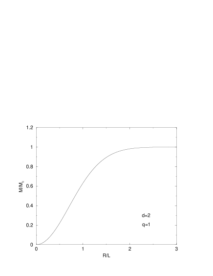
Figure 32: For box-confined systems, this figure represents the mass as a function of the central density (proportional to $(R/L)^{2}$) for $q=1$.

Figure 33: Density energy profile (in units of $c^{4}/8\pi GR^{2}$) for different values of the central density (proportional to $(R/L)^{2}$) for $q=1$. For $L\rightarrow 0$ or $\epsilon_{0}\rightarrow+\infty$, the density profile tends to a Dirac peak.

6.3 The Milne variables

The Milne variables are defined by Eqs. (178). Using the analytical solution (207), we find for $q\neq 1$ that

$$u=\frac{1}{q}(1-(\xi/\xi_{0})^{2})^{\frac{2}{1-q}},\quad v=\frac{q\xi^{2}}{1-(\xi/\xi_{0})^{2}}.$$ (229)

Eliminating $\xi$ between these two expressions, we obtain

$$v=q\xi_{0}^{2}\left[(qu)^{\frac{q-1}{2}}-1\right].$$ (230)

The $(u,v)$ curve is parametrized by $\xi$. For $\xi=0$, we have $(u,v)=(1/q,0)$ and for $\xi\rightarrow\xi_{0}$, we have $(u,v)=(0,+\infty)$. For $q=1$, using the analytical solution (217), we find that

$$u=e^{-\xi^{2}/2},\quad v=\xi^{2}.$$ (231)

Eliminating $\xi$ between these two expressions, we obtain

$$v=-2\ln u.$$ (232)

The $(u,v)$ curve is parametrized by $\xi$. For $\xi=0$, we have $(u,v)=(1,0)$ and for $\xi\rightarrow+\infty$, we have $(u,v)=(0,+\infty)$. The solution curve in the $(u,v)$ plane is represented in Fig. 34.

Figure 34: The $(u,v)$ curve of “isothermal” spheres in two-dimensional gravity for $q=1/2$ and $q=1$.

If the system is confined within a box of radius $R$, the previous results remain valid for $\xi\leq\alpha\leq\xi_{0}$ where

$$\alpha=\left\{\frac{8\pi G\epsilon_{0}(1+q)}{c^{4}q}\right\}^{1/2}R.$$ (233)

From the criterion (187), we can extrapolate that the condition of marginal stability in $d=2$ corresponds to $u_{0}=0$. Therefore, the solutions that are confined by a box are stable, since $u_{0}=u(\alpha)>0$, while the self-confined solutions are marginally stable since $u_{0}=u(\xi_{0})=0$.

7 Conclusion

In this paper, we have carried out a thorough analysis of the structure and stability of relativistic stars (and self-gravitating radiation) described by a linear equation of state. In order to prevent evaporation, we have placed these objects in a cavity. We have studied the stability of the steady states (i) by linearizing the Einstein equations around the stationary solution and studying the sign of the squared pulsation $\sigma^{2}$ (see Paper I) and (ii) by considering the sign of the second-order variations of the baryon number (see Appendix D). We have found analytically that the instability occurs precisely at the first mass peak when we vary the central density for a fixed box radius. We have applied these results to explicit examples: self-gravitating radiation, the core of neutron stars, stiffest stars, Zel’dovich model etc. We have determined their domains of stability precisely and found some upper bounds on the thermodynamical parameters like the entropy. We have obtained scaling laws (with a precise determination of the prefactor) that we compared with the scaling laws of black holes. We have stressed, however, that pure scaling laws correspond to unstable configurations and that they can hold only approximately close to the critical radius $R_{c}$. We have generalized our results in $d$ dimensions and found two critical dimensions. In $d=2$, steady state solutions exist for a unique value of the mass $M_{c}=c^{2}/(8G)$ and they can be obtained analytically. For this mass, we get an infinite family of solutions parametrized by the central density. The density profiles vanish at a finite radius for $q\neq 1$ and decrease as a Gaussian for $q=1$. These configurations are probably marginally stable. They may evolve dynamically either toward a completely spread profile (evaporation) or toward a Dirac peak (black hole) with mass $M_{c}$ (collapse). On the other hand, for $d\geq d_{crit}(q)$ (where $d_{crit}(q)$ is a nontrivial dimension depending on $q$), the mass vs central density profile no longer displays oscillations, and all the configurations of the series of equilibria are stable whatever their central density. In that case, the pure scaling laws are meaningful. The physical implication of this result needs further investigation. For the self-gravitating radiation, we have found that the critical dimension has the non-integer value $d_{crit}=9.96404372...$ This is an interesting (and intriguing) result because it results solely from the combination of the Einstein equations and the Stefan-Boltzmann law, so it has a relatively fundamental origin.

We have also shown that the structure of relativistic stars with a linear equation of state in general relativity is strikingly similar to the structure of isothermal stars in Newtonian gravity. Basically, the analogy stems from the resemblence between the general relativistic Emden equation and its Newtonian counterpart and the fact that they coincide for $q\rightarrow 0$. On the other hand, stable relativistic stars with a linear equation of state maximize the baryon number $N[\epsilon]$ at fixed mass-energy $M[\epsilon]$ (formal nonlinear dynamical stability for the Einstein equations). Similarly, isothermal stars in Newtonian gravity minimize the energy functional ${\cal W}[\rho]$ at fixed mass $M[\rho]$ (formal nonlinear dynamical stability for the Euler-Poisson system) or minimize the Boltzmann free energy functional $F_{B}[\rho]$ at fixed mass $M[\rho]$ (thermodynamical stability in the canonical ensemble). As a result, the curves of Figs. 1 and 4 are respectively similar to (i) the mass-versus-central density $M(\rho_{0})$ at fixed temperature and volume and (ii) the energy functional ${\cal W}(\rho_{0})$ or the Boltzmann free energy $F_{B}(\rho_{0})$-versus-central density at fixed temperature and volume for Newtonian isothermal spheres (Chavanis 2002d). On the other hand, by interpreting the mass $M[\epsilon]$ as an energy and the baryon number $N[\epsilon]$ as an entropy, the criterion of formal nonlinear dynamical stability in general relativity is equivalent to a criterion of thermodynamical stability in the microcanonical ensemble. Therefore, the curves of Figs. 8, 10, 11, and 15 are respectively similar to (i) the energy $E({\cal R})$ and the entropy $S({\cal R})$-versus-density contrast at fixed mass and volume, (ii) the entropy $S(E)$-versus-energy at fixed mass and volume, and (iii) the caloric curve $\beta(E)$ at fixed mass and volume for Newtonian isothermal spheres (Chavanis 2002d). Therefore, depending on the interpretation, relativistic stars with a linear equation of state share analogies with classical isothermal spheres in both microcanonical and canonical ensembles. These interesting analogies are intriguing and deserve further investigation.

Note added: Coincidentally, two other authors V. Vaganov [arXiv:0707.0864] and J. Hammersley [arXiv:0707.0961] have, in two recent papers, independently carried out studies of the self-gravitating radiation in $d$ dimensions (in an asymptotically anti-de Sitter space $\Lambda\leq 0$) related to the one developed in Sect. 5. These authors find that the oscillations in the mass-central density relation disappear above a critical dimension. On the basis of numerical calculations, J. Hammersley obtains a simple relation between the critical density $\epsilon_{0,c}$ and the dimension $d$ and argues that the critical dimension is $d_{crit}=10$ ($+1$ if we include time). Our analytical approach (for a cosmological constant $\Lambda=0$) is more precise and shows that the critical dimension corresponding to the self-gravitating radiation has the noninteger value $d_{c}=9.96404372...$ very close to $10$ (a minor mistake in calculation was made in the first version of this manuscript and led to a slightly different value for the critical dimension. This mistake was pointed out to me by V. Vaganov, who performed, in a new Appendix B of his paper [arXiv:0707.0864v4], a phase plane analysis of the Oppenheimer-Volkoff equation with $\Lambda=0$. This provides an alternative derivation of the asymptotic results obtained in our Sect. 5.4). Our approach also provides a thorough description of the structure and stability of relativistic stars with a linear equation of state $p=q\epsilon$ for any $q\in[0,1]$ and $d\geq 2$. Note that the existence of a critical dimension above which the oscillations of the mass-central density relation disappear had been noted previously in Sire & Chavanis (2002) for Newtonian isothermal spheres (corresponding to $q\rightarrow 0$). In that case, $d_{crit}=10$ exactly. The present study extends this work in general relativity.

Acknowledgements. I am grateful to Kalyana Rama for pointing out his work after a first version of this paper was placed on arXiv:0707.2292.

Appendix A Some elements of black hole thermodynamics

In this appendix, we recall elementary notions of black holes thermodynamics in order to facilitate the comparison with the results obtained in this paper.

In the seventies, different works (Christodoulou 1970, Penrose & Floyd 1971, Hawking 1971) have shown that the area $A=4\pi R^{2}$ of a black hole (more precisely the area of its event horizon) cannot decrease. Noting the analogy with the second law of thermodynamics, these results led Bekenstein (1973) to conjecture that black holes have an entropy proportional to their area $A=4\pi R^{2}$. On the basis of dimensional analysis, he obtained

$$S_{BH}=\lambda\frac{k_{B}A}{L_{P}^{2}},$$ (234)

where $\lambda$ is a dimensionless constant. If black holes have entropy and energy, they must possess a temperature. Hawking (1975) showed that black holes emit thermal radiation at a temperature

$$k_{B}T=\frac{\hbar c^{3}}{8\pi GM}.$$ (235)

Considering a Schwarzschild black hole for which

$$M=\frac{Rc^{2}}{2G},$$ (236)

and writing the first law of thermodynamics in the form

$$d(Mc^{2})=TdS_{BH},$$ (237)

one gets

$$k_{B}T=\frac{\hbar c^{3}}{32\pi\lambda GM}.$$ (238)

Comparing this expression with the expression of the Hawking temperature (235) it is found that $\lambda=1/4$. This leads to the following expression of the Black Hole (or Bekenstein-Hawking) entropy

$$S_{BH}=\frac{k_{B}A}{4L_{P}^{2}}.$$ (239)

On the other hand, using Eq. (236), the black hole temperature (238) can be written

$$k_{B}T=\frac{c\hbar}{4\pi R},$$ (240)

emphasising the scaling $T\sim 1/R$ with the radius. On the other hand, the energy $E=Mc^{2}$ of the black hole is related to its temperature by

$$E=\frac{\hbar c^{5}}{8\pi Gk_{B}T}.$$ (241)

Therefore, black holes have negative specific heats

$$C=\frac{dE}{dT}=-\frac{\hbar c^{5}}{8\pi Gk_{B}T^{2}}<0.$$ (242)

Appendix B The Tolman relation

Global thermodynamic equilibrium requires that the redshifted temperature $e^{\nu(r)/2}T(r)$ is uniform throughout the medium. This is called the Tolman (1934) relation

$$e^{\nu(r)/2}T(r)=T_{0},$$ (243)

where $T_{0}$ is a constant. Since $\nu(r)\rightarrow 0$ for $r\rightarrow+\infty$, we conclude that $T_{0}$ is the temperature measured by an observer at infinity. Let us check that this relation is satisfied by our equations. From Eq. (14), we find that

$$T(r)\propto\epsilon(r)^{q/(q+1)}.$$ (244)

On the other hand, according to Eq. (102) of Paper I, the Einstein equations for a spherically distribution of matter give

$$\frac{dP}{dr}=-\frac{1}{2}(\epsilon+P)\frac{d\nu}{dr}.$$ (245)

For the linear equation of state (8), this relation can be easily integrated into

$$\epsilon(r)=Ae^{-\frac{q+1}{q}\frac{\nu(r)}{2}},$$ (246)

where $A$ is a constant. Comparing Eqs. (244) and (246), we obtain the Tolman relation (243). Now, applying this relation at the boundary $r=R$ of the system, we obtain

$$e^{\nu(R)/2}T(R)=T_{0}.$$ (247)

On the other hand, according to Eq. (109) of Paper I, we have

$$\nu(R)=\ln(1-2GM/Rc^{2}).$$ (248)

Therefore, the temperature at infinity is related to the temperature at the surface of the star by

$$T_{0}=T(R)\sqrt{1-\frac{2GM}{Rc^{2}}}.$$ (249)

This relation shows that the thermodynamical temperature defined by Eq. (89) coincides with the temperature measured by an observer at infinity.

Appendix C The Newtonian limit in a $d$-dimensional universe

In this appendix, we briefly discuss the Newtonian limit of the Einstein equations in a $(d+1)$-dimensional space-time. Considering first the general relativistic Emden equations (147)-(148), the Newtonian limit corresponds to $q\rightarrow 0$. In that limit Eqs. (147)-(148) reduce to

$$\frac{d\psi}{d\xi}=(d-2)\frac{M(\xi)}{\xi^{d-1}},\quad{\rm and}\quad\frac{dM}{d\xi}=\xi^{d-1}e^{-\psi},$$ (250)

and they combine to give

$$\frac{1}{\xi^{d-1}}\frac{d}{d\xi}\left(\xi^{d-1}\frac{d\psi}{d\xi}\right)=(d-2)e^{-\psi}.$$ (251)

This is the familiar Emden equation (Chandrasekhar 1942) with an additional factor $d-2$. For $d>2$, we can rescale the parameters so as to recover the Emden equation exactly. For $d=2$, we see that there is no Newtonian limit in $d=2$. This can also be seen, more fundamentally, at the level of the Oppenheimer-Volkoff equations (135)-(136). The Newtonian limit corresponds to $c\rightarrow+\infty$. In that limit, Eq. (135) reduces to

$$\frac{dP}{dr}=-\frac{8\pi(d-2)}{(d-1)S_{d}}\rho\frac{GM(r)}{r^{d-1}}.$$ (252)

This is to be compared with the classical condition of hydrostatic equilibrium

$$\frac{dP}{dr}=-\rho\frac{G_{Newton}M(r)}{r^{d-1}}.$$ (253)

We find that the gravitational constants are related to each other by

$$G_{Newton}=\frac{(d-2)8\pi}{(d-1)S_{d}}G_{Einstein}.$$ (254)

They only coincide in $d=3$. In $d=1$, the Newtonian gravitational constant is infinite and it vanishes in $d=2$. Therefore, there is apparently no Newtonian limit in one- and two-dimensional gravity.

Appendix D Dynamical stability analysis

In this appendix, we consider the formal nonlinear dynamical stability of a box-confined relativistic star with a linear equation of state (8). Specifically, we study the maximization problem

$${\rm Max}\quad\{N[\epsilon]\quad|\quad M[\epsilon]=M\quad{\rm fixed}\},$$ (255)

and show that it provides the same condition of stability as the condition of linear dynamical stability studied in Paper I by considering the growth rate of a solution of the linearized Einstein equations. Therefore, linear and nonlinear dynamical stability coincide. Stability is lost when the mass-central density profile $M(\epsilon_{0})$ presents an extremum. The solutions on the series of equilibra $M(\epsilon_{0})$ are nonlinearly dynamically stable before the turning point of mass, and they become linearly dynamically unstable after the turning point of mass. This is similar to the case of barotropic stars described by the Euler-Poisson system in Newtonian gravity (Chavanis 2002a, 2002c, 2006).

D.1 The first-order variations

For a linear equation of state, using Eqs. (3) and (10), the baryon number can be expressed in terms of the energy density in the form

$$N=\left(\frac{q}{K}\right)^{1/\gamma}\int_{0}^{R}\epsilon^{\frac{1}{q+1}}\left[1-\frac{2GM(r)}{rc^{2}}\right]^{-1/2}4\pi r^{2}dr.$$ (256)

Therefore, the first-order variations of baryon number and mass are

$$\delta N=\left(\frac{q}{K}\right)^{1/\gamma}\int_{0}^{R}\epsilon^{\frac{1}{q+1}}\left[1-\frac{2GM(r)}{rc^{2}}\right]^{-1/2}$$

$$\times\left(\frac{1}{q+1}\frac{\delta\epsilon}{\epsilon}+\frac{\frac{G\delta M(r)}{rc^{2}}}{1-\frac{2GM(r)}{rc^{2}}}\right)4\pi r^{2}dr,$$ (257)

$$\delta M=\frac{4\pi}{c^{2}}\int_{0}^{R}\delta\epsilon r^{2}dr.$$ (258)

Substituting $\delta M(r)=\frac{4\pi}{c^{2}}\int_{0}^{r}\delta\epsilon r^{{}^{\prime}2}dr^{\prime}$ in Eq. (257), interchanging the order of the integrals, and writing the first-order condition as Eq. (5), we obtain

$$\int_{0}^{R}4\pi r^{2}dr\delta\epsilon\biggl{\{}\epsilon^{-\frac{q}{q+1}}\frac{1}{q+1}\left[1-\frac{2GM(r)}{rc^{2}}\right]^{-1/2}$$

$$+\frac{G}{c^{4}}\int_{r}^{R}\epsilon(r^{\prime})^{\frac{1}{q+1}}\left[1-\frac{2GM(r^{\prime})}{r^{\prime}c^{2}}\right]^{-3/2}4\pi r^{\prime}dr^{\prime}\biggr{\}}$$

$$-\mu\left(\frac{K}{q}\right)^{1/\gamma}\int_{0}^{R}\frac{4\pi}{c^{2}}\delta\epsilon r^{2}dr=0.$$ (259)

This condition must be true for all variations, implying

$$\mu\left(\frac{K}{q}\right)^{1/\gamma}\frac{1}{c^{2}}=\frac{1}{q+1}\epsilon^{-\frac{q}{q+1}}\left[1-\frac{2GM(r)}{rc^{2}}\right]^{-1/2}$$

$$+\frac{G}{c^{4}}\int_{r}^{R}\epsilon(r^{\prime})^{\frac{1}{q+1}}\left[1-\frac{2GM(r^{\prime})}{r^{\prime}c^{2}}\right]^{-3/2}4\pi r^{\prime}dr^{\prime}.$$ (260)

If we take $r=R$, we find that the value of $\mu$ is given by

$$\mu\left(\frac{K}{q}\right)^{1/\gamma}\frac{1}{c^{2}}=\frac{1}{q+1}\epsilon(R)^{-\frac{q}{q+1}}\left[1-\frac{2GM}{Rc^{2}}\right]^{-1/2}.$$ (261)

On the other hand, if we take the derivative of Eq. (260) with respect to $r$, we obtain, after simplification,

$$\left\{1-\frac{2GM(r)}{c^{2}r}\right\}\frac{d\epsilon}{dr}=-\frac{1}{c^{2}}\frac{q+1}{q}\epsilon\left\{\frac{GM(r)}{r^{2}}+\frac{4\pi Gq}{c^{2}}\epsilon r\right\},$$

(262)

which is the Oppenheimer-Volkoff equation (1) with a linear equation of state $P=q\epsilon$. This is a particular case of the general result given by Weinberg (1972) which is valid for an arbitrary equation of state provided that the perturbations are adiabatic.

D.2 The second-order variations

We now turn to the more complicated second-order variations. Writing

$$f=\delta M(r),\qquad\frac{df}{dr}=\frac{4\pi}{c^{2}}\delta\epsilon r^{2},$$ (263)

the second variations of the baryon number are given by

$$\delta^{2}N=\frac{G}{q+1}\int_{0}^{R}dr\frac{1}{r}\left[1-\frac{2GM(r)}{rc^{2}}\right]^{-3/2}\epsilon^{-\frac{q}{q+1}}f\frac{df}{dr}$$

$$+\frac{3G^{2}}{2c^{4}}\int_{0}^{R}dr4\pi\left[1-\frac{2GM(r)}{rc^{2}}\right]^{-5/2}\epsilon^{\frac{1}{q+1}}f^{2}$$

$$-\int_{0}^{R}dr\frac{c^{4}}{4\pi r^{2}}\frac{q}{2(q+1)^{2}}\left[1-\frac{2GM(r)}{rc^{2}}\right]^{-1/2}\epsilon^{-\frac{2q+1}{q+1}}\left(\frac{df}{dr}\right)^{2},$$

(264)

where we have omitted, for brevity, the positive term $(q/K)^{1/\gamma}$ in factor on the r.h.s. This is the sum of three integrals that will be denoted $I_{1}$, $I_{2}$, and $I_{3}$. Integrating by parts the first integral, we get

$$I_{1}+I_{2}=\int_{0}^{R}\biggl{\{}\frac{3G^{2}}{2c^{4}}4\pi\left[1-\frac{2GM(r)}{rc^{2}}\right]^{-5/2}\epsilon^{\frac{1}{q+1}}$$

$$-\frac{G}{2(q+1)}\frac{d}{dr}\left(\frac{1}{r}\left[1-\frac{2GM(r)}{rc^{2}}\right]^{-3/2}\epsilon^{-\frac{q}{q+1}}\right)\biggr{\}}f^{2}dr.$$

(265)

Expanding the derivative, we obtain

$$I_{1}+I_{2}=\frac{G}{4(q+1)}\int_{0}^{R}\frac{1}{r^{2}}\left[1-\frac{2GM(r)}{rc^{2}}\right]^{-3/2}\epsilon^{-\frac{q}{q+1}}$$

$$\times\biggl{\{}\frac{24\pi G}{c^{4}}\left[1-\frac{2GM(r)}{rc^{2}}\right]^{-1}q\epsilon r^{2}+\frac{2qr}{q+1}\frac{1}{\epsilon}\frac{d\epsilon}{dr}$$

$$+3\left[1-\frac{2GM(r)}{rc^{2}}\right]^{-1}-1\biggr{\}}f^{2}dr.\qquad$$ (266)

Using the Oppenheimer-Volkoff equation (262), we find after simplification

$$I_{1}+I_{2}=\frac{G}{4(q+1)}\int_{0}^{R}\frac{1}{r^{2}}\left[1-\frac{2GM(r)}{rc^{2}}\right]^{-3/2}\epsilon^{-\frac{q}{q+1}}$$

$$\times\biggl{(}2-\frac{4qr}{q+1}\frac{1}{\epsilon}\frac{d\epsilon}{dr}\biggr{)}f^{2}dr.\qquad$$ (267)

On the other hand, integrating by parts the third integral in Eq. (264) and using the Oppenheimer-Volkoff equation (262), we obtain after simplification

$$I_{3}=\frac{c^{4}}{8\pi}\frac{q}{(q+1)^{2}}\int_{0}^{R}drf\frac{1}{r^{2}}\left[1-\frac{2GM(r)}{rc^{2}}\right]^{-1/2}$$

$$\times\epsilon^{-\frac{2q+1}{q+1}}\biggl{[}\frac{d^{2}f}{dr^{2}}+\frac{df}{dr}\biggl{\{}-\frac{2}{r}-\frac{1}{\epsilon}\frac{d\epsilon}{dr}$$

$$+\biggl{[}1-\frac{2GM(r)}{rc^{2}}\biggr{]}^{-1}\frac{4\pi G}{c^{4}}(q+1)\epsilon r\biggr{\}}\biggr{]}.$$ (268)

In conclusion,

$$\delta^{2}N=\frac{G}{2(q+1)}\int_{0}^{R}\frac{1}{r^{2}}e^{3\lambda/2}\epsilon^{-\frac{q}{q+1}}\biggl{(}1-\frac{2qr}{q+1}\frac{1}{\epsilon}\frac{d\epsilon}{dr}\biggr{)}f^{2}dr$$

$$+\frac{c^{4}}{8\pi}\frac{q}{(q+1)^{2}}\int_{0}^{R}drf\frac{1}{r^{2}}e^{\lambda/2}\epsilon^{-\frac{2q+1}{q+1}}$$

$$\times\biggl{[}\frac{d^{2}f}{dr^{2}}+\frac{df}{dr}\left\{-\frac{2}{r}-\frac{1}{\epsilon}\frac{d\epsilon}{dr}+e^{\lambda}\frac{4\pi G}{c^{4}}(q+1)\epsilon r\right\}\biggr{]}.$$

(269)

To determine the sign of $\delta^{2}N$, we are led to consider the eigenvalue equation

$$\frac{c^{4}}{8\pi}\frac{q}{(q+1)^{2}}\frac{1}{r^{2}}e^{\lambda/2}\epsilon^{-\frac{2q+1}{q+1}}$$

$$\times\biggl{[}\frac{d^{2}f}{dr^{2}}+\frac{df}{dr}\left\{-\frac{2}{r}-\frac{1}{\epsilon}\frac{d\epsilon}{dr}+e^{\lambda}\frac{4\pi G}{c^{4}}(q+1)\epsilon r\right\}\biggr{]}$$

$$+\frac{G}{2(q+1)}\frac{1}{r^{2}}e^{3\lambda/2}\epsilon^{-\frac{q}{q+1}}\biggl{(}1-\frac{2qr}{q+1}\frac{1}{\epsilon}\frac{d\epsilon}{dr}\biggr{)}f=\Lambda f,$$ (270)

with the boundary conditions $f(0)=f(\alpha)=0$ (see Paper I). Introducing the variables defined in Sect. 2.3, the foregoing equation can be rewritten as

$$\frac{d^{2}f}{d\xi^{2}}+\left\{-\frac{2}{\xi}+\frac{d\psi}{d\xi}+q\xi e^{\lambda-\psi}\right\}\frac{df}{d\xi}$$

$$+e^{\lambda-\psi}\biggl{(}1+\frac{2q\xi}{q+1}\frac{d\psi}{d\xi}\biggr{)}f$$

$$=\frac{qc^{4}}{2\pi G^{2}}\epsilon_{0}^{-\frac{1}{q+1}}\xi^{2}e^{-\lambda/2}e^{-\frac{2q+1}{q+1}\psi}\Lambda f,$$ (271)

with $f(0)=f(\alpha)=0$. This equation determines a discrete set of eigenvalues $\Lambda_{1}>\Lambda_{2}>\Lambda_{3}$, … If all the eigenvalues $\Lambda$ are negative, then $\delta^{2}N\leq 0$ and the configuration is a maximum of $N$ at fixed mass. If at least one eigenvalue is positive, the configuration is an unstable saddle point. We therefore need to determine the point of marginal stability $\Lambda=0$ in the series of equilibria. It is obtained by solving the differential equation

$$\frac{d^{2}f}{d\xi^{2}}+\left\{-\frac{2}{\xi}+\frac{d\psi}{d\xi}+q\xi e^{\lambda-\psi}\right\}\frac{df}{d\xi}$$

$$+e^{\lambda-\psi}\biggl{(}1+\frac{2q\xi}{q+1}\frac{d\psi}{d\xi}\biggr{)}f=0,$$

(272)

with $f(0)=f(\alpha)=0$. The same equation was obtained in Paper I [see Eq. (167)] by determining the condition of marginal linear dynamical stability. Therefore, the thresholds of linear and nonlinear dynamical stability coincide. Equation (272) was solved in Paper I and led to the relation (I-171) identical to (I-148). Therefore, the points where $\Lambda=0$ correspond to extrema of mass in the series of equilibria $M(\alpha)$. A first eigenvalue $\Lambda_{1}$ becomes positive at the first mass peak (implying instability), and new modes of stability are lost at subsequent extrema. At the $i$-th extremum, we have $\Lambda_{1}>\Lambda_{2}>...>\Lambda_{i}=0>\Lambda_{i+1}>\Lambda_{i+2}>...$.

References

- (1) Antonov, V.A. 1962, Vest. Leningr. Gos. Univ., 7, 135
- (2) Banks, T., & Fischler, W. 2001, [hep-th/0111142]
- (3) Banks, T., Fischler, W., Kashani-Poor, A., McNees, R., & Paban, S. 2002, Class. Quantum Grav., 19, 4717
- (4) Bekenstein, J.D. 1973, PRD, 7, 2333
- (5) Bekenstein, J.D. 1981, PRD, 23, 287
- (6) Bousso, R. 2002, Rev. Mod. Phys., 74, 825
- (7) Chandrasekhar, S. 1942, An Introduction to the Theory of Stellar Structure (Dover)
- (8) Chandrasekhar, S. 1972, “A limiting case of relativistic equilibrium” in General Relativity, papers in honour of J.L. Synge, Edited by L.O’ Raifeartaigh (Oxford)
- (9) Chavanis, P.H. 2002a, A&A, 381, 340
- (10) Chavanis, P.H. 2002b, A&A, 381, 709 (Paper I)
- (11) Chavanis, P.H. 2002c, A&A, 386, 732
- (12) Chavanis, P.H. 2002d, PRE, 65, 056123
- (13) Chavanis, P.H. 2004, PRE, 69, 066126
- (14) Chavanis, P.H. 2006a, A&A, 451, 109
- (15) Chavanis, P.H. 2006b, C. R. Physique, 7, 331
- (16) Chavanis, P.H. 2006c, Int J. Mod. Phys. B , 20, 3113
- (17) Chavanis, P.H. 2007a, PRD, 76, 023004
- (18) Chavanis, P.H. 2007b, Physica A, 384, 392
- (19) Chavanis, P.H., & Rieutord, M. 2003, A&A, 412, 1
- (20) Chavanis, P.H., & Sire, C. 2004, PRE, 69, 016116
- (21) de Vega, H.J., & Sanchez, N. 2002, Nucl. Phys. B, 625, 409
- (22) Christodoulou, D. 1970, PRL, 25, 1596
- (23) Hawking, S. 1971, PRL 26, 1344
- (24) Hawking, S. 1975, Commun. math. Phys. 43, 199
- (25) Hertel, P., & Thirring, W. 1971, Commun. math. Phys. 24, 22
- (26) ’t Hooft, G. 1985, Nucl. Phys. B 256, 727
- (27) Kalyana Rama, S. 2007, Phys. Lett. B 645, 365
- (28) Katz, J. 1978, MNRAS 183, 765
- (29) Katz, J. 2003, Found. Phys. 33, 223
- (30) Klein, O. 1947, Ark. Mat. Astr. Fys. 34, 19
- (31) Landau, L.D., & Lifshitz, E.M. 1960, The classical theory of fields (Fizmatgiz)
- (32) Lynden-Bell, D., & Wood, R. 1968, MNRAS 138, 495
- (33) Meltzer, D.W., & Thorne, K.S. 1966, ApJ 145, 514
- (34) Misner, C.W., & Zapolsky, H.S. 1964, Phys. Rev. Lett. 12, 635
- (35) Oppenheim, J. 2002, Phys. Rev. D 65, 024020
- (36) Oppenheimer, J.R., & Volkoff, G.M. 1939, Phys. Rev. 55, 374
- (37) Padmanabhan, T. 1990, Phys. Rep. 188,285
- (38) Penrose, R., & Floyd, R.M. 1971, Nature, 229, 177
- (39) Pesci, A. 2007, Class. Quantum Grav. 24, 2283
- (40) Ponce de Leon, J., & Cruz, N. 2000, Gen. Relativ. Gravit. 32, 1207
- (41) Schmidt, H.J., & Homann, F. 2000, Gen. Relativ. Gravit. 32, 919
- (42) Sire, C., & Chavanis, P.H. 2002, PRE, 66, 046133
- (43) Sorkin, R.D., Wald, R.M., & Jiu, Z.Z. 1981, Gen. Relativ. Gravit. 13, 1127
- (44) Srednicki, M. 1993, Phys. Rev. Lett. 71, 666
- (45) Tolman, R.C. 1934, Relativity, Thermodynamics and Cosmology (Oxford: Clarendon)
- (46) Tsallis, C. 1988, J. Stat. Phys. 52, 479
- (47) Weinberg, S. 1972, Gravitation and Cosmology (John Wiley)
- (48) Zel’dovich, Ya.B. 1962, Soviet Phys. J.E.T.P. 14, 1143