Integer partitions and exclusion statistics: Limit shapes and the largest part of Young diagrams

Abstract

We compute the limit shapes of the Young diagrams of the minimal difference $p$ partitions and provide a simple physical interpretation for the limit shapes. We also calculate the asymptotic distribution of the largest part of the Young diagram and show that the scaled distribution has a Gumbel form for all $p$. This Gumbel statistics for the largest part remains unchanged even for general partitions of the form $E=\sum_{i}n_{i}i^{1/\nu}$ with $\nu>0$ where $n_{i}$ is the number of times the part $i$ appears.

Journal-ref: J. Stat. Mech. (2007) P10001

 

 

1 Introduction

Exclusion statistics [1, 2, 3, 4, 5, 6, 7, 8]—a generalization of Bose and Fermi statistics—can be defined in the following thermodynamical sense. Let $Z(\beta,z)$ denote the grand partition function of a quantum gas of particles at inverse temperature $\beta$ and fugacity $z$. Such a gas is said to obey exclusion statistics with parameter $0\leq p\leq 1$, if $Z(\beta,z)$ can be expressed as an integral representation

$$\ln Z(\beta,z)=\int_{0}^{\infty}{\tilde{\rho}}(\epsilon)\ln y_{p}\left(z\rme^{-\beta\epsilon}\right)\,\rmd\epsilon,$$ (1)

where ${\tilde{\rho}}(\epsilon)$ denotes a single particle density of states and the function $y_{p}(x)$, which encodes fractional statistics, is given by the solution of the equation

$$y_{p}(x)-x\,y_{p}^{1-p}(x)=1.$$ (2)

In the cases $p=0$ and $p=1$, substituting $y_{p}(x)$ explicitly in (1) yield the standard grand partition functions of non-interacting bosons and fermions respectively. The fractional exclusion statistics with parameter $0<p<1$ (that corresponds to an interacting gas) smoothly interpolates between these two extreme cases. Two known microscopic quantum mechanical realizations of exclusion statistics are the Lowest Landau Level (LLL) anyon model [2, 3] and the Calogero model [6, 7], with ${\tilde{\rho}}(\epsilon)$ being, respectively, the LLL density of states and the free one-dimensional density of states.

It is well known that a gas of non-interacting bosons ($p=0$) or fermions ($p=1$) occupying a single particle equidistant spectrum both have a combinatorial interpretation in terms of the integer partition problem [9]. A partition of a positive integer $E$ is a decomposition of $E$ as a sum of a nonincreasing sequence of positive integers $\{h_{j}\}$, i.e., $E=\sum_{j}h_{j}$ such that $h_{j}\geq h_{j+1}$, for $j=1,2\ldots$. For example, $4$ can be partitioned in $5$ ways: $4$, $3+1$, $2+2$, $2+1+1$, and $1+1+1+1$. Partitions can be graphically represented by Young diagrams (also called Ferrers diagrams), where $h_{j}$ corresponds to the height of the $j$-th column (see figure 1).

Figure 1: (a) All the Young diagrams for the partitions of 4. (b) The Young diagram of the partition $91=18+16+13+13+9+6+5+5+3+3$, and the corresponding configuration of non-interacting bosons occupying energy levels $\epsilon_{i}=i$ for $i=1,2,\ldots,18$.

In the Young diagram of a given partition of $E$, if $n_{i}$ denotes the number of columns having heights equal to $i$, then clearly $E=\sum_{i}n_{i}\epsilon_{i}$ —which can now be interpreted as the total energy of a non-interacting quantum gas of bosons where $\epsilon_{i}=i$ for $i=1,2,\ldots,\infty$ represent equidistant single particle energy levels and $n_{i}=0,1,2,\ldots,\infty$ represents the occupation number of the $i$-th level (see figure 1(b)). On the other hand, if one expresses a positive integer $E$ as a sum of strictly decreasing sequence of positive integers, i.e. $E=\sum_{j}h_{j}$ such that $h_{j}>h_{j+1}$ (e.g. allowed partitions of 4 are: $4$ and $3+1$), then the restricted partition problem corresponds to a non-interacting quantum gas of fermions, for which $n_{i}=0,1$. In the partitioning problems if one restricts the number of summands to be $N$, then clearly $N=\sum_{i}n_{i}$ represents the total number of particles. For example, if $E=4$ and $N=2$, the allowed partitions are $3+1$ and $2+2$ in the unrestricted problem, whereas the only allowed restricted partition is $3+1$. The number $\rho(E,N)$ of ways of partitioning $E$ into $N$ parts is simply the micro-canonical partition function of a gas of quantum particles with total energy $E$ and total number of particles $N$:

$$\rho(E,N)=\sum_{\{n_{i}\}}\delta\left(E-\sum_{i=1}^{\infty}n_{i}\epsilon_{i}\right)\,\delta\left(N-\sum_{i=1}^{\infty}n_{i}\right).$$ (3)

The grand partition functions, i.e., $Z(\beta,z)=\sum_{N}\sum_{E}z^{N}\rme^{-\beta E}\rho(E,N)$, for the unrestricted and restricted partitions are $Z(\beta,z)=\prod_{i=1}^{\infty}(1-z\rme^{-\beta i})^{-1}$ and $Z(\beta,z)=\prod_{i=1}^{\infty}(1+z\rme^{-\beta i})$ and hence $\ln Z(\beta,z)$ in the limit $\beta\rightarrow 0$ and $\tilde{\rho}(\epsilon)=1$ reduce to (1) with $p=0$ and $p=1$ respectively.

Unlike Bose and Fermi statistics which describes non-interacting particles, for a quantum gas obeying exclusion statistics with parameter $0<p<1$, it is a priori not obvious how to provide a combinatorial description, since the underlying physical models with exclusion statistics describe interacting systems. However it has recently been shown [10] that a combinatorial description of exclusion statistics is possible in terms of a generalized partition problem known as the minimal difference $p$ partition (MDP–$p$), which we will define in the next section. Even though the parameter $p$ in MDP–$p$ is an integer, in [10] it has been shown that, when one analytically continues the results to non-integer values of $p$, for $0<p<1$, and in the limit $\beta\to 0$, the MDP–$p$ corresponds to a gas of quantum particles obeying exclusion statistics. This correspondence between exclusion statistics and MDP–$p$ motivates us to investigate some other aspects of the MDP–$p$ problem in this paper.

2 Problems and outline

Figure 2: A typical Young diagram for MDP–$p$ problem. The thick solid border shows the height profile. $W_{h}$ is the width of the Young diagram at a height $h$, i.e., $W_{h}$ is the number of columns whose heights $\geq h$.

In the MDP–$p$ problem, a positive integer $E$ is expressed as a sum of positive integers $E=\sum_{j}h_{j}$ such that $h_{j}-h_{j+1}\geq p$ (see figure 2). Therefore, $p=0$ corresponds to unrestricted partitions and $p=1$ to restricted partitions into distinct parts. The shortest part in the MDP–$p$ problem is usually taken to be $\geq 1$. However, for the calculation of certain specific quantities in this model, it is useful to consider a somewhat generalized version with the shortest part $\geq s$, where $s$ is considered to be a variable. The grand partition function of this problem was obtained recently in [10], which is given by (1) with constant density of states ${\tilde{\rho}}(\epsilon)=1$ and the lower limit of integration being $s$.

One may also think of the MDP–$p$ in terms of a quantum system consisting of equidistant energy levels $\epsilon_{i}=i$ for $i=1,2,\ldots,\infty$. Now a given height $h_{j}=i$ corresponds the energy level $\epsilon_{i}=i$ and the number of columns with height $i$ is the occupation number $n_{i}$. Since the difference between two consecutive heights in the MDP–$p$ must be at least $p$, the gap between two adjacent occupied energy levels must be at least $p$. Clearly for $p=0$ this gap is zero, and hence each level can be occupied by any number of particles (bosons). For $p=1$, each level can be occupied by at most one particle (fermions). Again for $p>1$ a level can be occupied by at most one particle. However, in this case, when a energy level is occupied by a particle, the adjacent $p-1$ levels must remain unoccupied.

One major issue in the partition problem is to study the limit shape, i.e., the average height profile of an ensemble of Young diagrams with a fixed but large $E$. The shape (height profile) can be defined by the width $W_{h}$ of the Young diagram at a height $h$ (see figure 2). In other words, $W_{h}$ is the number of columns of the Young diagram whose height is greater than or equal to $h$. In this corresponding quantum system, $W_{h}$ represents the total number of particles occupying energy levels above $h$.

The height profile of the Young diagram of the unrestricted partition ($p=0$) was first studied by Temperley, who was interested in determining the equilibrium profile of a simple cubic crystal grown from the corner of three walls at right angles. The two dimensional version of the problem —where walls (two) are along the horizontal and the vertical axes and $E$ “bricks” (molecules) are packed into the first quadrant one by one such that each brick, when it is added, makes two contact along faces— corresponds to the $p=0$ partition problem. Temperley [11] computed the equilibrium profile of this two dimensional crystal. More recently the investigation of the limit shape of random partitions has been developed extensively by Vershik [12, 13, 14] and collaborators. The case of uniform random partitions was treated by Vershik who proved for the bosonic ($p=0$) as well as the fermionic ($p=1$) case that the rescaled $h/\sqrt{E}$ vs. $W_{h}/\sqrt{E}$ curves converge to limiting curves when $E\rightarrow\infty$, and obtained these limit shapes explicitly. These results were extended by Romik [15] to the MDP–$p$ for $p=2$. In this paper we compute the following two quantities:

1. The limit shape of the Young diagrams of the MDP–$p$ for any $p$, from which the previously obtained results for $p=0,1,2$ follow as special cases.

2. The distribution of the largest part of the Young diagrams of the MDP–$p$ problem for all $p$, whereas the earlier result existed only for the $p=0$ case [16].

The average height profile $\langle W_{h}\rangle$ of the Young diagrams of the partitions of a given integer $E$ is easier to compute in the grand canonical ensemble. Therefore one requires a restricted grand partition function $Z_{h}(\beta,z)$ which counts the columns whose heights $\geq h$, and the full grand partition function $Z(\beta,z)$ which counts all the columns. From the restricted grand partition function one finds $\langle W_{h}\rangle=z\frac{\partial}{\partial z}\ln Z_{h}(\beta,z)|_{z=1}$. For given large $E$, the parameter $\beta$ is fixed by the relation $E=-\frac{\partial}{\partial\beta}\ln Z(\beta,1)$.

On the other hand, to compute the number of partitions $\rho_{p}(E,l)$ of an integer $E$ such that the largest part $\leq l$, it is useful to consider the partition function $Z_{l}(\beta)=\sum_{E}\rme^{-\beta E}\rho_{p}(E,l)$ first. Formally $\rho_{p}(E,l)$ can be obtained by inverting $Z_{l}(\beta)$ with respect to $\beta$, and for large $E$ the asymptotic behavior of $\rho_{p}(E,l)$ is obtained from the saddle point approximation, where the parameter $\beta$ is fixed in terms of given $E$ by the saddle point relation $E=-\frac{\partial}{\partial\beta}\ln Z_{l}(\beta)$.

Thus, it is useful to consider a more general restricted grand partition function $Z(\beta,z,l,s)$ that counts the columns whose heights lie between $s$ and $l$. All the other partition functions we need for our calculations can be obtained from $Z(\beta,z,l,s)$ by taking various limits on $s$ and $l$. For example, by putting $s=1$ and taking the limit $l\rightarrow\infty$ one obtains $Z(\beta,z)$. Similarly $s=h$ and the limit $l\rightarrow\infty$ gives $Z_{h}(\beta,z)$ and putting $s=1$ and $z=1$ gives $Z_{l}(\beta)$. As we will see later in (14) and (23) that $\beta\sim E^{-1/2}$ for large $E$. Therefore, hereafter we will work in the limit $\beta\rightarrow 0$.

The rest of the paper is organized as follows. We first obtain the generalized grand partition function $Z(\beta,z,l,s)$ of the MDP–$p$ problem in the next section. In section 4 we compute the limit shapes of the Young diagrams and also provide a simple physical interpretation of the result. In section 5 we calculate the distribution of the largest part of the MDP–$p$ . Finally, we conclude with a summary and some remarks in section 6.

3 Restricted grand partition function of MDP–$p$ problem

Let $\rho_{p}(E,N,l,s)$ be the number of ways of partitioning an integer $E$ into $N$ parts in the MDP–$p$ problem such that the largest part is at most $l$ and the smallest part is at least $s$, i.e., $E=\sum_{j=1}^{N}h_{j}$ such that $h_{1}\leq l$, $h_{j+1}\leq h_{j}-p$ for all $j=1,2,\ldots,N-1$, and $h_{N}\geq s$. Then clearly, $[\rho_{p}(E,N,l,s)-\rho_{p}(E,N,l-1,s)]$ gives the number of MDP–$p$ of $E$, such that the largest part is exactly equal to $l$, and smallest part is at least $s$. Now, by eliminating the first part $h_{1}=l$ from the partition one immediately realizes that the above number is precisely $\rho_{p}(E-l,N-1,l-p,s)$, i.e., the number of MDP–$p$ of $E-l$ into $N-1$ parts such that the largest part is at most $l-p$ and the smallest part is at least $s$. Therefore, one has the recursion relation

$$\rho_{p}(E,N,l,s)=\rho_{p}(E,N,l-1,s)+\rho_{p}(E-l,N-1,l-p,s).$$ (4)

Following similar reasoning one can also derive another recursion relation in terms of the smallest part $s$,

$$\rho_{p}(E,N,l,s)=\rho_{p}(E,N,l,s+1)+\rho_{p}(E-s,N-1,l,s+p).$$ (5)

It follows from (4) and (5) that the grand partition function $Z(\beta,z,l,s)=\sum_{N}\sum_{E}z^{N}\rme^{-\beta E}\rho_{p}(E,N,l,s)$ satisfies the recursion relations:

$$Z(\beta,z,l,s)=Z(\beta,z,l-1,s)+z\rme^{-\beta l}Z(\beta,z,l-p,s),$$ (6)

$$Z(\beta,z,l,s)=Z(\beta,z,l,s+1)+z\rme^{-\beta s}Z(\beta,z,l,s+p).$$ (7)

From these equations, it is evident that in the scaling limit $\beta\rightarrow 0$, and both $s$ and $l$ large, the correct scaling variables are $\beta s$ and $\beta l$, so that $\beta s$ and $\beta l$ remain finite. One knows from the statistical mechanics that the free energy $\beta^{-1}\ln Z(\beta,z,l,s)$ becomes a function of the only the scaling variables in the limit $\beta\rightarrow 0$. Therefore in this limit it is natural to expect

$$Z(\beta,z,l,s)\approx\exp\left(\frac{1}{\beta}\Phi(\beta l,\beta s,z)\right).$$ (8)

Now to determine the scaling function $\phi(\beta l,\beta s,z)$, we substitute the ansatz (8) in (6) and (7), and then expand $\Phi(\beta l-\beta,\beta s,z)$ and $\Phi(\beta l-\beta p,\beta s,z)$ about $\beta l$, and $\Phi(\beta l,\beta s+\beta,z)$ and $\Phi(\beta l,\beta s+\beta p,z)$ about $\beta s$, respectively in Taylor series up to first order, which yields the equations:

$$\qquad\exp(-\Phi_{\beta l}) +z\rme^{-\beta l}\exp(-p\Phi_{\beta l}) =1,\quad\mbox{where}\quad\Phi_{\beta l}=\frac{\partial}{\partial u}\Phi(u,\beta s,z)\Big{|}_{u=\beta l},$$ (9)

$$\qquad\exp(\Phi_{\beta s}) +z\rme^{-\beta s}\exp(p\Phi_{\beta s}) =1,\quad\mbox{where}\quad\Phi_{\beta s}=\frac{\partial}{\partial v}\Phi(\beta l,v,z)\Big{|}_{v=\beta s}.$$ (10)

It is evident from (9) and (10), that $\Phi_{\beta l}$ and $\Phi_{\beta s}$ are function of the arguments $z\rme^{-\beta l}$ and $z\rme^{-\beta s}$ respectively, and the solutions are

$$\Phi_{\beta l}=\ln\,y_{p}\left(z\rme^{-\beta l}\right)\quad\mbox{and}\quad\Phi_{\beta s}=-\ln\,y_{p}\left(z\rme^{-\beta s}\right)$$ (11)

where $y_{p}(x)$ satisfies the equation $y_{p}(x)-x\,y_{p}^{1-p}(x)=1$, which is the same equation (2) one encounters in exclusion statistics. Equation (11) implies, $\Phi(u,v,z)=\int_{v}^{u}\ln y_{p}\left(z\rme^{-\epsilon}\right)\,\rmd\epsilon.$ Therefore, (8) yields

$$\ln Z(\beta,z,l,s)=\frac{1}{\beta}\int_{\beta s}^{\beta l}\ln y_{p}\left(z\rme^{-\epsilon}\right)\,\rmd\epsilon,$$ (12)

i.e. (1) with constant density of states ${\tilde{\rho}}(\epsilon)=1$, and the lower and upper limits of integration being $s$ and $l$ respectively. This is the key equation, using which we compute the limit shapes and the largest parts of the Young diagrams in section 4 and section 5 respectively. The limit $\beta l\rightarrow\infty$ also provides a simpler derivation of an earlier result [10], which showed a link between the exclusion statistics and the MDP–$p$ problem.

4 Limit shapes of Young diagrams

Let us consider all the MDP–$p$ of an integer $E$ with uniform measure. Then the number of columns having height between $s$ and $l$, averaged over all the Young diagrams of the MDP–$p$ of $E$, is obtained from (12) as

$$\qquad\left\langle N_{s}^{l}(z)\right\rangle=z\frac{\partial}{\partial z}\ln Z(\beta,z,l,s)=\frac{1}{\beta}\left[\ln y_{p}\left(z\rme^{-\beta s}\right)-\ln y_{p}\left(ze^{-\beta l}\right)\right].$$ (13)

Now to obtain the parameter $\beta$ in terms of the given large integer $E$ one again uses (12) with the limits $\beta l\rightarrow\infty$, $\beta s\rightarrow 0$, and $z=1$, i.e.,

$$\qquad E=-\frac{\partial}{\partial\beta}\ln Z(\beta,1,\infty,0)=\frac{b^{2}(p)}{\beta^{2}},\quad\mbox{where}\quad b^{2}(p)=\int_{0}^{\infty}\ln y_{p}\left(\rme^{-\epsilon}\right)\,\rmd\epsilon$$ (14)

is a constant which depends on the parameter $p$.

The average shape or the height profile of the Young diagrams $\langle W_{h}\rangle$ is simply given by (13) with $s=h$, $l\rightarrow\infty$ and $z=1$, i.e.,

$$\beta\left\langle W_{h}\right\rangle=\ln y_{p}\left(\rme^{-\beta h}\right),\quad\mbox{where}\quad\beta=\frac{b(p)}{\sqrt{E}}.$$ (15)

For instance for $p=0,1$ and $2$, solving (2) yields $y_{0}(x)=1/(1-x)$, $y_{1}(x)=(1+x)$, and $y_{2}(x)=\left[1+\sqrt{1+4x}\right]/2$ respectively. From which using (14) one finds $b(0)=\pi/\sqrt{6}$, $b(1)=\pi/\sqrt{12}$ and $b(2)=\pi/\sqrt{15}$ in agreement with the earlier known results [12, 15].

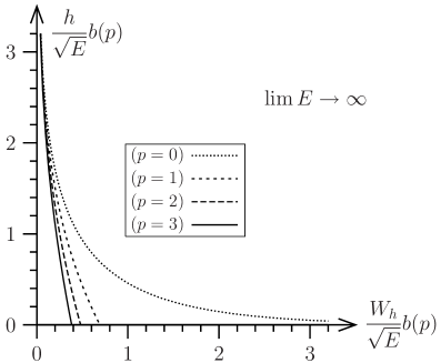
Figure 3: Limit shapes for the minimal difference $p$ partitions with $p=0,1,2$, and $3$, where $b(0)=\pi/\sqrt{6}$, $b(1)=\pi/\sqrt{12}$, $b(2)=\pi/\sqrt{15}$, and $b(3)=0.752617\ldots$.

The fluctuation about the average shape can be computed from (12) using

$$\langle W_{h}^{2}\rangle-\langle W_{h}\rangle^{2}=z\frac{\partial}{\partial z}z\frac{\partial}{\partial z}\ln Z(\beta,z,\infty,h)\Big{|}_{z=1},$$ (16)

which gives

$$\beta^{2}\left[\langle W_{h}^{2}\rangle-\langle W_{h}\rangle^{2}\right]=\beta\rme^{-\beta h}\left[\frac{y_{p}^{\prime}\left(\rme^{-\beta h}\right)}{y_{p}\left(\rme^{-\beta h}\right)}\right],$$ (17)

where $y_{p}^{\prime}(x)$ denotes the derivative of $y_{p}(x)$ with respect to its argument. This formula shows that the random variable $\beta W_{h}$ is strongly peaked around its mean value. Therefore, the curve $W_{h}/\sqrt{E}$ as a function of $h/\sqrt{E}$ converges to a limit curve when $E\rightarrow\infty$ (strictly speaking, to prove the existence of a limit curve, one needs to show that all the moments around the mean vanish when $E\rightarrow\infty$, which Vershik [13] showed for $p=0$ and $p=1$). Therefore hereafter we may replace $\langle\beta W_{h}\rangle$ by $\beta W_{h}$.

Using (2) and (15), one can express $h$ in terms of $W_{h}$ as,

$$h=-\frac{1}{\beta}\ln\left(1-\rme^{-\beta W_{h}}\right)-pW_{h}.$$ (18)

Introducing the scaling variables $x=W_{h}/\sqrt{E}$ and $y=h/\sqrt{E}$, using (14) and taking $E\rightarrow\infty$, yields the equation of the limit shape

$$y=-\frac{1}{b(p)}\ln(1-\rme^{-xb(p)})-px.$$ (19)

Figure 3 shows the limit shapes for the MDP–$p$ with $p=0,1,2$, and $3$.

Figure 4: (a) Transposed Young diagram for the unrestricted partition $91=18+16+13+13+9+6+5+5+3+3$. (b) Represents (a) in terms of non-interacting bosons (represented by ○) occupying energy levels $\epsilon_{i}=i$ for $i=1,2,\ldots,10$. (c) The configuration obtained from the bosonic configuration (b) by transferring particles from the higher levels to the lower levels such that in the final configuration all the levels below the highest occupied level $\epsilon_{5}=5$ receive 2 new particles (represented by ●) each, where ○represents the particles originally present in the initial bosonic configuration. (d) The Young diagram corresponding to the configuration (c). This is the transposed Young diagram of the partition $49=18+14+9+7+1$, in the minimal difference 2 partition problem.

Equation (18) has a simple physical interpretation which we explain below. For $p=0$, any transposed Young diagram (see figure 4) provides a valid unrestricted partition. Therefore the transposed diagram also corresponds to a non interacting system of bosons occupying single particle equidistant energy levels. However this is no more true when $p>0$. In this case the transposed Young diagram(see figure 4) corresponds to a quantum system where there is a certain energy level (which differs from one realization to another) which is occupied by at least one particle, and above which all the levels are empty, and below which each of the levels must be occupied by at least $p$ particles. Therefore, $h$ in the limit shape expression (18) represents the number of particles above the energy level $W_{h}$. For bosons with total energy $E$, this number is precisely given by (18) with $p=0$ and $\beta$ has to be determined in terms of $E$. Now, a configuration for $p>0$, can be obtained from a bosonic configuration by transferring particles from the higher energy levels to the lower ones such that, in the final configuration, levels below the highest occupied level (which has at least one particle) receive exactly $p$ new particles each. Clearly, in the final configuration obtained by this procedure, each of the levels below the highest occupied level has at least $p$ particles. However, since transferring a particle from a higher energy level to a lower one decreases energy of the system, to obtain a configuration for $p>0$ with energy $E$ requires the initial bosonic configuration to be at a higher energy (i.e., lower inverse temperature $\beta$) than $E$. Now, while going from a initial bosonic configuration to a configuration for $p>0$, one transfers total of $pW_{h}$ particles from the levels above $W_{h}$ to below (i.e., $p$ particles to each level), the average number number of particles above level $W_{h}$ decreases from the corresponding bosonic system ($p=0$) precisely by $pW_{h}$, which is exactly the content of (18) . In fact, $\beta$ in (18) can directly be determined by using condition $h\geq 0$ and the normalization $\int_{0}^{W_{h}^{*}}h\left(W_{h}\right)\,\rmd W_{h}=E$, where $W_{h}^{*}$ is the solution of the equation $h\left(W_{h}^{*}\right)=0$. Writing $\exp\left(\beta W_{h}^{*}\right)=y^{*}$, it satisfies $y^{*}-y^{*1-p}=1$, and in terms of $y^{*}$ one finds

$$\beta=\frac{b(p)}{\sqrt{E}}\quad\mbox{with}\quad b^{2}(p)=\frac{\pi^{2}}{6}-\mathrm{Li_{2}}(1/y^{*})-\frac{p}{2}(\ln y^{*})^{2},$$ (20)

where $\mathrm{Li_{2}}(z)=\sum_{k=1}^{\infty}z^{k}k^{-2}$ is the dilogarithm function. The expression for $b(p)$ in (20) also follows directly from its integral representation given in (18).

5 Largest part of Young diagrams

Equation (12) also allows one to compute the distribution of the largest part (i.e., the largest height in the Young diagram) in the MDP–$p$ problem. Let $\rho_{p}(E,l)$ be the number of partitions of the integer $E$ in MDP–$p$ problem, such that the largest part is at most $l$. Clearly, $\rho_{p}(E)=\rho_{p}(E,l\rightarrow\infty)$ gives the total number of partitions of $E$ and since the partitions are distributed with a uniform measure $C_{p}(l|E)=\rho_{p}(E,l)/\rho_{p}(E)$ gives the cumulative distribution of the largest height $l$. Note that the partition function $Z_{l}(\beta)=\sum_{E}\rme^{-\beta E}\rho_{p}(E,l)$ in the limit $\beta\rightarrow 0$ is obtained from (12) by simply taking the limit $\beta s\rightarrow 0$ and $z=1$. Therefore, formally inverting the Laplace transform (in the limit $\beta\rightarrow 0$, the sum over $E$ in the partition function of $Z_{l}(\beta)$ can be replaced by an integral), one can write

$$\rho_{p}(E,l)=\frac{1}{2\pi i}\int_{\gamma-i\infty}^{\gamma+i\infty}\exp\left[S_{E,l}(\beta)\right]\,\rmd\beta,$$ (21)

where $\gamma$ is a real constant chosen such that all singularities of integrand are to the left of the vertical contour in the complex plane, and the action

$$S_{E,l}(\beta)=\beta E+\frac{1}{\beta}\int_{0}^{\beta l}\ln y_{p}\left(\rme^{-\epsilon}\right)\,\rmd\epsilon.$$ (22)

For large $E$, the leading asymptotic behavior of $\rho_{p}(E,l)$ can be obtained from the saddle point approximation. Maximizing the action with respect to $\beta$, i.e., setting $\partial S/\partial\beta=0$ gives the saddle point equation

$$\beta^{2}E=\int_{0}^{\beta l}\ln y_{p}\left(\rme^{-\epsilon}\right)\,\rmd\epsilon-\beta l\ln y_{p}\left(\rme^{-\beta l}\right).$$ (23)

For large $E$, the saddle point $\beta^{*}$ is obtained implicitly solving the above equation and by substituting it back in the action $S_{E,l}(\beta^{*})$. Thus, to leading order,

$$\rho_{p}(E,l)\approx\exp\left[S_{E,l}(\beta^{*})\right],$$ (24)

where $S_{E,l}(\beta^{*})$ can be written as

$$S_{E,l}(\beta^{*})\approx\frac{1}{\beta^{*}}\left[2\int_{0}^{\beta^{*}l}\ln y_{p}\left(\rme^{-\epsilon}\right)\,\rmd\epsilon-\beta^{*}l\ln y_{p}\left(\rme^{-\beta^{*}l}\right)\right].$$ (25)

It is evident from the above equations that, in terms of $l$ and $E$, one has the scaling form $S_{E,l}(\beta^{*})=\sqrt{E}\,g_{p}(l/\sqrt{E})$, where the scaling function $g_{p}(x)$ can be determined as follows. We set $l/\sqrt{E}=x$ and $\beta^{*}l=H_{p}(x)$. In terms of these scaling variables, from the saddle point solution of (23) and the entropy (25) one has

$$\frac{H_{p}^{2}(x)}{x^{2}} =\int_{0}^{H_{p}(x)}\ln y_{p}\left(\rme^{-\epsilon}\right)\,\rmd\epsilon-H_{p}(x)\ln y_{p}\left(\rme^{-H_{p}(x)}\right),$$ (26)

and $$g_{p}(x) =2\frac{H_{p}(x)}{x}+x\ln y_{p}\left(\rme^{-H_{p}(x)}\right),$$ (27)

respectively. Thus, given $x$, one has to find $H_{p}(x)$ by implicitly solving (26), then substitute it back in (27) to get $g_{p}(x)$, and finally

$$\rho_{p}(E,l)\approx\exp\left[\sqrt{E}\,g_{p}\left(\frac{l}{\sqrt{E}}\right)\right].$$ (28)

For large $x$, using (26) and (27), it can be shown that

$$g_{p}(x)\approx 2b(p)-\frac{1}{b(p)}\exp\left[-b(p)x\right]\qquad\mbox{as}\quad x\rightarrow\infty,$$ (29)

where $b(p)$ is given in (14) and (20). Thus, from (28), $\rho_{p}(E)=\rho_{p}(E,l\rightarrow\infty)\sim\exp[2b(p)\sqrt{E}]$ to leading order for large $E$, which is the generalization of the Hardy-Ramanujan formula [17] for $\rho_{0}(E)$, provided by Meinardus [18]. The normalized cumulative distribution of $l$, i.e., $C_{p}(l|E)=\rho_{p}(E,l)/\rho_{p}(E)$, for large $E$ and $l\gg\sqrt{E}$, is therefore

$$C_{p}(l|E)\approx\exp\left[-\frac{\sqrt{E}}{b(p)}\exp\left(-\frac{b(p)}{\sqrt{E}}l\right)\right]=F\left(\frac{b(p)}{\sqrt{E}}\Bigl{[}l-l^{*}(E)\Bigr{]}\right),$$ (30)

where the characteristic value of $l$ is $l^{*}(E)=[\sqrt{E}/b(p)]\ln(\sqrt{E}/b(p))$, and the scaling function has the Gumbel form, $F(z)=\exp[-\exp[-z]]$. The result for the $p=0$ case, i.e., for $C_{0}(l|E)$, was first derived Erdös and Lehner [16]. Equation (30) provides a generalization of their result, which is valid for all $p$. The probability distribution $P_{p}(l|E)=C_{p}(l|E)-C_{p}(l-1|E)\approx{\partial C_{p}(l|E)}/{\partial l}$, obtained from (30),

$$\quad P_{p}(l|E)\approx\frac{b(p)}{\sqrt{E}}\,F^{\prime}\left(\frac{b(p)}{\sqrt{E}}\Bigl{[}l-l^{*}(E)\Bigr{]}\right),\quad\mbox{where}\quad F^{\prime}(z)=\exp[-z-\exp[-z]],$$ (31)

is highly asymmetric around the peak at $l=l^{*}(E)$. This limiting distribution describes the probability of typical fluctuations of $\Or(\sqrt{E})$ of the random variable $l$ around the peak $l^{*}(E)$.

6 Summary and remarks

In summary, we have obtained a generalized grand partition function for the minimal difference $p$ partition (MDP–$p$) of a positive integer $E$, where smallest part is at least $s$ and largest part is at most $l$, in the scaling limit $\beta\propto E^{-1/2}\rightarrow 0$, in terms of the scaling variables $\beta l$ and $\beta s$. The limit $\beta l\rightarrow\infty$ also provides a simpler derivation of an earlier result [10], which showed a link between the exclusion statistics and the MDP–$p$ problem, by showing that both problems are described by the same grand partition function in the limit $\beta\rightarrow 0$. Using the grand partition function we have computed the limiting shape of the Young diagram of the MDP–$p$ problem for all $p$, and also provided a simple physical interpretation of the result. Although the Young diagram is defined only for integer values of $p$, one can analytically continue the expression (15) for the width $W_{h}$ of the Young diagram to noninteger values of $p$. For $0<p<1$, $W_{h}$ corresponds to the number of particles each of which has energy at least $h$, in a system where the particles obeys exclusion statistics. We have also obtained the asymptotic distribution of the largest part of the Young diagram and showed that the scaled distribution has a Gumbel form for all $p$. When one analytically continues, for $0<p<1$, the largest part corresponds to the highest occupied energy level in exclusion statistics.

Note that for $p=0$, the transposed Young diagram of a given partition gives another valid $p=0$ partition. This symmetry implies that the statistics of the largest part is the same as the statistics of the number of parts in the $p=0$ partition problem. The distribution of the number of parts for $p=0$ was computed by Erdös and Lehner [16] and in the appropriate scaling limit it has a Gumbel form. However, the symmetry between the number of parts and the largest part no longer holds when $p>0$, where the distribution of the number of parts become Gaussian (see [10] and references therein).

Recently, the statistics of the number of parts for a general partitions of the form $E=\sum n_{i}i^{1/\nu}$ that corresponds to having a power-law density of states, $\tilde{\rho}(\epsilon)\sim\epsilon^{\nu-1}$, has been studied [19] in the bosonic sector ($p=0$). Clearly, $\nu=1$ corresponds to the usual unrestricted partition problem, where the number of parts obey Gumbel statistics. Interestingly, for $\nu\neq 1$, the authors in [19] also obtained the other two universal distribution laws of extreme value statistics, namely the Fréchet and Weibull distributions for $0<\nu<1$ and $\nu>1$ respectively.

Therefore, the general partition problem can be defined in the parameter space of $(\nu,p)$ with $\nu>0$ and $p\geq 0$. In this parameter space the point $(\nu=1,p=0)$ is a very special one at which both the number of parts and the largest part obey the same statistics given by the Gumbel distribution. Along the line $\nu=1$, the limiting distribution of the number of parts becomes Gaussian as soon as $p>0$, whereas the limiting distribution of the largest part remains Gumbel for all $p$, as we have shown in this paper. On the other hand, along the $p=0$ line, for the number of parts one finds [19] all the three universal laws of the extreme value statistics, for the parameter $0<\nu<1$, $\nu=1$, and $\nu>1$ respectively. Therefore, it is interesting to ask whether there is any region in the $(\nu,p)$ parameter space, where the largest part obeys another statistics than the Gumbel one. The answer is negative. For a general density of states, (22) includes a factor of $\tilde{\rho}(\epsilon/\beta)$ in the integrand. Following the similar steps provided afterwards, it can be shown that even for the power-law density of states $\tilde{\rho}(\epsilon)\sim\epsilon^{\nu-1}$, the scaled distribution of the largest part remains Gumbel in the whole $(\nu,p)$ plane. Thus, the largest part obeys a more robust law, in contrast to the number of parts.

Note added in proof

We thank K. Hikami for pointing out [20] in which the author obtained the solution of a recursion relation similar to (6) with $s=0$ for arbitrary $\beta$. However, for the purpose of this paper we require the solution only in the limit $\beta\rightarrow 0$. In this limit it is simpler to obtain it using the method presented in this paper rather than obtaining by taking the limit $\beta\rightarrow 0$ in the solution of [20]. The average occupation number at a level $i$ for the exclusion statistics has been studied in [2, 3, 4, 21, 22], which also can be obtained from (13) simply through

$$\langle n_{i}\rangle=-\frac{\partial}{\partial s}\left\langle N_{s}^{l}(z)\right\rangle\Big{|}_{s=i}=\frac{\partial}{\partial l}\left\langle N_{s}^{l}(z)\right\rangle\Big{|}_{l=i},$$ (32)

which via elementary algebra yields

$$\langle n_{i}\rangle=\left(\frac{1}{y_{p}(z\rme^{-\beta i})-1}+p\right)^{-1}$$ (33)

References

References

- [1] Haldane F D M 1991 “Fractional statistics” in arbitrary dimensions: A generalization of the Pauli principle Phys. Rev. Lett. 67 937
- [2] Dasnières de Veigy A and Ouvry S 1994 Equation of state of an anyon gas in a strong magnetic field Phys. Rev. Lett. 72 600
- [3] Dasnières de Veigy A and Ouvry S 1995 One-dimensional statistical mechanics for identical particles: the Calogero and anyon cases Mod. Phys. Lett. B 9 271
- [4] Wu Y S 1994 Statistical distribution for generalized ideal gas of fractional-statistics particles Phys. Rev. Lett. 73 922
- [5] Murthy M V N and Shankar R 1994 Haldane exclusion statistics and second virial coefficient Phys. Rev. Lett. 72 3629
- [6] Murthy M V N and Shankar R 1994 Thermodynamics of a one-dimensional ideal gas with fractional exclusion statistics Phys. Rev. Lett. 73 3331
- [7] Isakov S B 1994 Fractional statistics in one dimension: modeling by means of interaction and statistical mechanics Int. J. Mod. Phys. A 9 2563
- [8] Bergère M C 2000 Fractional statistic J. Math. Phys. 41 7252
- [9] Andrews G E 1998 The Theory of Partitions (Cambridge University Press, Cambridge)
- [10] Comtet A, Majumdar S N and Ouvry S 2007 Integer partitions and exclusion statistics J. Phys. A: Math. Theor. 40 11255
- [11] Temperley H N Y 1952 Statistical mechanics and the partition of numbers: the form of crystal surfaces Proc. Cambridge Philos. Soc. 48 683
- [12] Vershik A M 1996 Statistical mechanics of combinatorial partitions and their limit shapes Funct. Anal. Appl. 30 90
- [13] Freiman G, Vershik A M and Yakubovich Yu V 2000 A local limit theorem for random strict partitions Theory Probab. Appl 44 453
- [14] Vershik A M and Yakubovich Yu V 2001 The limit shape and fluctuations of random partitions of naturals with fixed number of summands Moscow Math. J. 1 457
- [15] Romik D 2003 Identities arising from limit shapes of constrained random partitions Preprint
- [16] Erdös P and Lehner J 1951 The distribution of the number of summands in the partitions of a positive integer Duke Math. J. 8 335
- [17] Hardy G H and Ramanujan S 1918 Asymptotic formulaæ in combinatory analysis Proc. London. Math. Soc. 17 75
- [18] Meinardus G 1954 Über partitionen mit differenzenbedingungen Math. Zeitschr. 61 289
- [19] Comtet A, Leboeuf P and Majumdar S N 2007 Level density of a Bose gas and extreme value statistics Phys. Rev. Lett. 98 070404
- [20] Hikami K 1995 Character and TBA for an ideal -on gas Phys. Lett. A 205 364
- [21] Hikami K 1998 Statistical mechanical interpretation of the inverse scattering method: level dynamics for exclusion statistics Phys. Rev. Lett. 80 4374
- [22] Hikami K 2000 Exclusion statistics and chiral partition function Physics and Combinatorics (Proc. Nagoya 2000 Int. Workshop) ed A N Kirillov and N Liskova (Singapore: World Scientific) pp 22–48