Rectification by charging – the physics of contact-induced current asymmetry in molecular conductors

Abstract

We outline the qualitatively different physics behind charging-induced current asymmetries in molecular conductors operating in the weakly interacting self-consistent field (SCF) and the strongly interacting Coulomb Blockade (CB) regimes. A conductance asymmetry arises in SCF because of the unequal mean-field potentials that shift a closed-shell conducting level differently for positive and negative bias. A very different current asymmetry arises for CB due to the unequal number of open-shell excitation channels at opposite bias voltages. The CB regime, dominated by single charge effects, typically requires a computationally demanding many-electron or Fock space description. However, our analysis of molecular Coulomb Blockade measurements reveals that many novel signatures can be explained using a simpler orthodox model that involves an incoherent sum of Fock space excitations and hence treats the molecule as a metallic dot or an island. This also reduces the complexity of the Fock space description by just including various charge configurations only, thus partially underscoring the importance of electronic structure, while retaining the essence of the single charge nature of the transport process. We finally point out, however, that the inclusion of electronic structure and hence well-resolved Fock space excitations is crucial in some notable examples.

I Introduction

Ever since its inception avi , molecular rectification continues to be of great practical interest. While rectification could arise from asymmetries in the intrinsic molecular structure or vacuum barriers at the ends, there are multiple experiments rei1 ; jpark ; rscott that exhibit pronounced asymmetries in current voltage (I-V) or conductance voltage (G-V) characteristics due to unequal coupling with contacts. Fig. 1 shows that the nature of contact-induced asymmetry is qualitatively different depending on the nature of the molecule-contact bonding. For molecules strongly coupled with the contacts with adiabatic charge addition, equal current plateaus are reached over unequal SCF voltage widths (Fig. 1a), leading to prominent conductance asymmetries rei1 . The origin of this asymmetry is the different average charging energies that generate unequal mean-field potentials for opposite bias voltages rasymm . Reducing the contact-molecular coupling drives the system into CB, where the intermediate open-shell current values are also asymmetric rralph2 (Fig. 1b). This asymmetry has a different physical origin rooted in its many-body excitations, driven by the unequal number of discrete charge addition and removal channels at opposite bias. It is thus clear that the physics of rectification can differ widely depending on the strength of the electron-electron interaction.

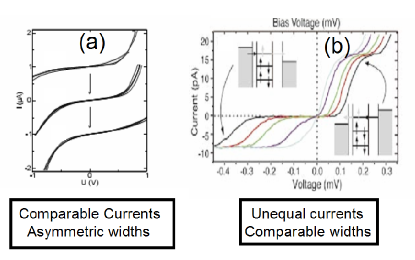
Figure 1: (Color online) Experiments showing (a) comparable currents reached over unequal voltage widths rei1 in the SCF limit; (b) unequal currents with comparable widths in the CB limit rralph2 .

The non-equilibrium Green’s function (NEGF) formalism is widely established for treating quantum transport in the SCF regime, for a whole variety of materials from nanoscale silicon transistors to molecules, nanowires, nanotubes and spintronic elements. The ability to incorporate sophisticated quantum chemical models max_dft ; damle2 through averaged potentials makes the NEGF-SCF scheme particularly attractive in the community. What is not widely appreciated is that this approach does not readily translate to the CB regime, even qualitatively rbhasko ; rbhaskob ; rbhaskoc . The CB regime, observed in molecules with weak contact coupling jpark ; rscott , manifests clear signatures of single-electron charging such as suppressed zero-bias conductances and abrupt jumps in current. Although several approximate treatments max_dft_2 ; rpal ; ssan ; pals have been suggested to handle CB within effective one-electron potentials, the inherent difficulty arises from the fact that the open-shell current levels depend on full exclusion statistics in its many-body Fock space. Even for a minimal single-orbital model, it is easy to establish that while the open-shell current plateau widths depend on the correlation strengths, their heights are independent of correlation and, in that sense, universal rbhasko . The transport problem in CB maps onto a rather difficult combinatorial problem in many-body space that is hard to capture a-priori through a one-particle SCF potential, or improve upon phenomenologically.

It seems likely that in the limit of weak coupling to contacts a proper treatment of the above excitations will require solving a set of master equations directly in the Fock space of the molecular many-body Hamiltonian rbhasko ; rhettler . A significant penalty is the increased computational cost that requires sacrificing the quantum chemical sophistication of ab-initio models in lieu of an exact treatment of the Coulomb interaction in simpler, phenomenological models. Within such an exactly diagonalizable model, one can capture transport features quite novel and unique to the CB regime, such as inelastic cotunneling, gate-modulated current rectification and Pauli spin blockade rbhasko2 ; rbhasko ; rsiddiqui . The presence of contact asymmetry makes these features even more intriguing, while somewhat simplifying the analysis by effectively driving the system into equilibrium with the stronger contact.

In this paper, we first identify the origin of current asymmetry with a minimal system of a single spin degenerate energy doublet, employing NEGF in the SCF limit and master equations for sequential tunneling rralph in the CB limit (we refer to this as a “Fock-space” CB model). We then extend this “Fock-space model” to a general molecular Hamiltonian to explain how multiple orbitals in CB allow simultaneous sequential tunneling into excited states, making the conductance peak heights vary with gate voltage. We also explain the origin of exchange in conductance peak asymmetry by the neutral and singly charged molecule. While this Fock space model involves a computationally intensive, exactly diagonalized many-body Hamiltonian about the charge degeneracy point arising from the different excitation spectra accessed, in many cases a simpler approximation works. Our analysis of the experimental trends in the CB regime reveals that many of the novel signatures such as gate dependence of conductance peaks and asymmetry flipping can be explained using a simpler “orthodox model” that involves an incoherent sum of Fock space excitations. We conclude by pointing out some limitations of such a simplified approach, as well as possible applications that may need careful attention to the detailed excitation spectrum.

II Origin of Current Asymmetries – The essential physics

As mentioned earlier, there are two distinct physical limits of transport. In the SCF limit, contact broadenings $\Gamma$ are greater than or comparable with the single electron charging $U$. In the opposite CB limit $U\gg\Gamma$ and single-electron charging dominates. Conductance asymmetries in both regimes of transport have been experimentally observed in molecular conduction. While there are ways to handle each regime separately, treatments are inherently perturbative, with an approximate treatment of correlation (in terms of $U/\Gamma$) for the SCF regime, and an approximate treatment of broadening (in terms of $\Gamma/U$) for the CB regime. The lack of a small parameter in the intermediate coupling regime ($U\sim\Gamma$) makes the exact treatment of transport, even for a simple model system, potentially intractable rbhaskob .

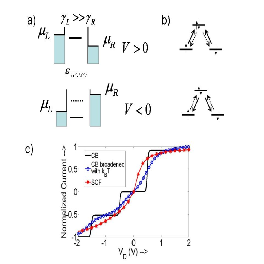
Figure 2: (Color Online) Origin of Current Asymmetries: a) In the SCF regime (stars), when $\gamma_{L}\gg\gamma_{R}$ for $V>0$, the left contact keeps the HOMO $\epsilon_{HOMO}$ level filled to its neutral charge making conduction possible, while for $V<0$, the left contact empties the electron leading to the level floating out of the bias window, creating unequal plateau widths for opposite bias. b) In the CB regime (bold solid line) however, for $V<0$, charge removal process by the right contact is rate determining and occurs in two different ways, while for $V>0$, charge addition process is rate determining and occurs in only one way. This leads to asymmetry in plateau heights along the two bias directions. c) While the transition between the two limits is hard to accomplish correctly, a phenomenological broadening through an artificial enhanced temperature (circles) illustrates how the open-shell intermediate CB plateau morphs into a higher effective broadening, restoring the SCF result in the limit of $\Gamma\gg U$

The origin of asymmetric I-Vs can be easily elucidated with a minimal model for current conduction through a spin degenerate, filled (closed-shell) molecular level doublet. We assume equal capacitive couplings but unequal resistive couplings to the contacts, so that the molecular level shifts by half the applied Laplace potential and the current onsets arise symmetrically around zero bias. In the SCF limit, contact asymmetry results in equal currents adiabatically smeared out over a larger voltage width along one bias direction than the other. This charging based asymmetry has been experimentally seen rei1 , and can be intuitively rationalized as follows. Consider a spin degenerate energy level, a highest occupied molecular orbital (HOMO) for example, that is fully occupied at equilibrium. For asymmetric contact couplings $\gamma_{L}\gg\gamma_{R}$, charge addition dominates for positive bias on the right contact and removal for negative bias, as shown in Fig. 2(a). For positive bias the energy level is maintained at neutrality by the dominant left contact and the current flow through the level is determined by the removal rate. Along reverse bias, in contrast, charge removal by the left contact drives the system away from neutrality towards a net positive charge, whose Coulomb cost floats the level out of the bias window. This means that a larger bias is needed to fully conduct through the level, dragging out the I-V in that direction. The direction of the asymmetry flips if conduction is through the lowest unoccupied molecular orbital (LUMO) instead. Notably the peak currents and initial plateau onsets remain the same along both directions, but their complete saturations are delayed by different amounts.

The origin and manifestation of current asymmetry is qualitatively different in the CB limit, where charge addition or removal is abrupt and in integer amounts. Given asymmetric contact couplings ($\gamma_{L}\gg\gamma_{R}$), the left contact adds (removes) an electron as soon as the right contact removes (adds) it, so that the rate determining step becomes the dynamics of the weaker right contact. For positive bias, charge removal can happen in two ways, from $\uparrow\downarrow$ to $\uparrow$ and $\downarrow$, while for opposite bias the right contact can add a spin in only one way, either $\uparrow$ or $\downarrow$ to $\uparrow\downarrow$. This scheme of charge transfer (Fig. 2b) leads to twice the current step for positive bias than negative rralph ; rralph2 .

An important question is whether one can smoothly transition from the CB to the SCF asymmetry by progressively increasing the broadening. While this is hard to do exactly owing to the inherent difficulty involved in the broadening many-particle states rWacker , for the purpose of illustration one can add various degrees of approximate broadening rappenzeller . We choose to do this by increasing the temperature and incorporating this through Boltzmann factors in the many-body occupancies rgerhard . As seen in Fig. 2(c), this approximate treatment morphs the CB asymmetry into the very different version seen for the SCF limit. For negative bias on the weaker contact, ‘shell-filling’ rzung of the HOMO level with a net positive charge creates a CB plateau that is missing in its positive bias ‘shell-tunneling’ counterpart. This extra CB plateau gets encased by the broadened manifold, leading to the postponed conduction seen in the SCF limit. It is worth mentioning though that the correspondence is only qualitative and is observed to worsen for higher onset voltages, underscoring the inadequacy of thermal effects and possibly other phenomenological ways to incorporate broadening in correlated systems, particularly in the near equal coupling, non-equilibrium limit which combines shell tunneling with shell filling.

III Coulomb Blockade Formalism: Fock-space vs Orthodox

In this paper, we focus mainly on the CB regime. The object of this section is to present the formalism in detail, beginning with the one that employs the Fock space. Here, one needs to keep track not only of various ground state charge configurations, but also various excitations within each charge state. Following that we derive the orthodox model that integrates out the effect of excitations in an incoherent way. A discussion of merits and de-merits of such a simplification comprises the subsequent sections.

III.1 Fock-Space Master Equation

The starting point is a molecular many-body Hamiltonian

$$\hat{H} = \sum_{m}\epsilon_{m}n_{m}+\sum_{m\neq p}t_{mp}c_{m}^{\dagger}{c_{p}}$$ (1)

$$+ \sum_{m}U_{mm}n_{m\uparrow}n_{m\downarrow}+\frac{1}{2}\sum_{m\neq p}U_{mp}n_{m}n_{p},$$

where $m,p$ denote the spin-charge basis functions within a tight binding formulation, with $\epsilon,t$ and $U$ denoting on-site, hopping and charging terms, respectively. Exactly diagonalizing this Hamiltonian yields a large spectrum of closely spaced excitations in every charged molecular configuration. The lead molecule exchange processes are accounted for within the sequential tunneling approximation timm ; rbraig . This results in a set of master equation that involve transition rates $R_{(N,i)\rightarrow(N\pm 1,j)}$ between states differing by a single electron. If one neglects off-diagonal coherences, the master equation rbraig is cast in terms of the occupation probabilities $P^{N}_{i}$ of each N electron many-body state $|N,i\rangle$ with total energy $E^{N}_{i}$. The end result is a set of independent equations defined by the size of the Fock space rralph

$$\frac{dP^{N}_{i}}{dt}=-\sum_{j}\left[R_{(N,i)\rightarrow(N\pm 1,j)}P^{N}_{i}-R_{(N\pm 1,j)\rightarrow(N,i)}P^{N\pm 1}_{j}\right]$$ (2)

along with the normalization equation $\sum_{i,N}P^{N}_{i}=1$. For weakly coupled dispersionless contacts, parameterized using bare-electron tunneling rates $\gamma_{\alpha}$ ($\alpha$: left/right contact) within a Golden Rule treatment, we define the transition-resolved rate constants

$$\Gamma_{ij\alpha}^{Nr} = \gamma_{\alpha}|\langle N-1,j|c_{\alpha}|N,i\rangle|^{2}$$

$$\Gamma_{ij\alpha}^{Na} = \gamma_{\alpha}|\langle N+1,j|c^{\dagger}_{\alpha}|N,i\rangle|^{2},$$ (3)

where $c^{\dagger}_{\alpha},c_{\alpha}$ are the creation/annihilation operators for an electron on the left or right molecular end atom coupled with the corresponding electrode. The transition rates are given by

$$R_{(N,i)\rightarrow(N-1,j)} = \sum_{\alpha=L,R}\Gamma_{ij\alpha}^{Nr}\left[1-f(\epsilon^{Nr}_{ij}-\mu_{\alpha})\right]$$

$$R_{(N-1,j)\rightarrow(N,i)} = \sum_{\alpha=L,R}\Gamma_{ij\alpha}^{Nr}f(\epsilon^{Nr}_{ij}-\mu_{\alpha}).$$ (4)

for the removal levels $(N,i\rightarrow N-1,j)$, and replacing $(r\rightarrow a,f\rightarrow 1-f)$ for the addition levels $(N,i\rightarrow N+1,j)$. $\mu_{\alpha}$ are the contact electrochemical potentials, $f$ is the corresponding Fermi function, with single particle removal and addition transport channels $\epsilon^{Nr}_{ij}=E^{N}_{i}-E^{N-1}_{j}$, and $\epsilon^{Na}_{ij}=E^{N+1}_{j}-E^{N}_{i}$. Finally, the steady-state solution to Eq. (2) is used to get the left terminal current

$$I=\pm\frac{e}{\hbar}\sum_{N,ij}\left[R^{L}_{(N,i)\rightarrow(N\pm 1,j)}P^{N}_{i}-R^{L}_{(N\pm 1,j)\rightarrow(N,i)}P^{N\pm 1}_{j}\right]$$ (5)

where $R^{L}$ includes the contributions to $R$ from the left contact alone. In the equation above, states corresponding to a removal of electrons by the left electrode involve a negative sign. We usually calculate current in a break-junction configuration with equal electrostatic coupling with the leads, $\mu_{L,R}=E_{F}\mp eV_{d}/2$.

III.2 The Orthodox Model

In the previous sub-section, the computational complexity of the master equation defined in Eq. (2) arises from the need to keep track of not only charge $N$, but also all configurational degrees of freedom $i$. Thus the evaluation of transition rates defined in Eq. (4) and eventually current (Eq. 5) depends on our knowledge of various many-electron wavefunctions $|N,i\rangle$ and total energies $E^{N}_{i}$. The “orthodox” theory of single-electron tunneling, however, does not distinguish between excitation levels rsold ; rkorot . Note also that in the orthodox theory, the junctions are generally denoted by $(1,2)$ instead of $(L,R)$. Eq. (5) then becomes

$$I = \pm\frac{e}{\hbar}\sum_{N}\left[R_{N\rightarrow{N\pm 1}}^{(1)}-R_{N\rightarrow{N\mp 1}}^{(1)}\right]P^{N}$$ (6)

$$= \pm\frac{e}{\hbar}\sum_{N}\left[R_{N\rightarrow{N\mp 1}}^{(2)}-R_{N\rightarrow{N\pm 1}}^{(2)}\right]P^{N}$$ (7)

We have simplified the second term in the summation using a simple change of variables. Let us assume incoherent processes that introduce an additional exclusion term in the transition process (appendix). Then a “golden-rule” calculation gives

$$R_{N\rightarrow{N+1}}^{(2)} =\int_{-\infty}^{\infty}{\displaystyle{2\pi}}\Gamma_{2}^{Na}D_{2}(E-\mu_{2})f(E-\mu_{2})$$ (8)

$$\times D_{m}(E-\mu)\left[1-f(E-\mu)\right]dE\mbox{, }$$

where $D_{2}(E)$ and $D_{m}(E)$ are the densities of states of the right and middle electrodes, and $\mu$ is the Fermi energy of the molecular system. If the level separation between one-electron levels is very small, like in a metallic quantum dot, the densities of states are approximately constant for the calculation of the removal and addition rates. By additionally assuming $\Gamma_{\alpha}^{Na}$ is energy-independent, Eq. (8) simplifies:

$$R_{N\rightarrow{N\pm 1}}^{(j)}=\frac{\hbar}{R_{j}e^{2}}\left(\frac{-\Delta E_{j}^{\pm}}{1-exp(\Delta E_{j}^{\pm}/kT)}\right)\mbox{, }$$ (9)

where $R_{j}$ is the junction resistance. $\Delta E_{j}^{\pm}$ is the transition energy corresponding to adding or removing an electron at the $j^{th}$ contact; from simple electrostatics,

$$\Delta E_{1}^{\pm}=\Delta U^{\pm}\mp\frac{eC_{2}}{C_{\Sigma}}V_{D}\mp\frac{eC_{G}}{C_{\Sigma}}V_{G},$$

$$\Delta E_{2}^{\pm}=\Delta U^{\pm}\pm\frac{eC_{1}}{C_{\Sigma}}V_{D}\mp\frac{eC_{G}}{C_{\Sigma}}V_{G},$$ (10)

where $C_{1,2,G}$ and $C_{\Sigma}$ are the terminal and total capacitances respectively, $V_{D}$ and $V_{G}$ are drain and gate voltages respectively, and $\Delta U^{\pm}$ is the Coulomb offset for the addition or removal of an electron. Notice that we now have a simpler analytical and closed form solution to our set of master equations, using our trick of summing over excitations. In doing so, we also brought in simpler circuit parameters such as junction resistance and capacitance that aid in our analytical understanding of threshold voltages and current magnitudes.

When considering the “orthodox” Coulomb Blockade theory in the regime of strong contact asymmetry ($R_{2}\gg R_{1}$), it is illuminating - and not overly limiting - to consider what happens at very low temperatures. Following the analysis of Hanna and Tinkham Han91 , at low temperatures the ensemble distribution of electrons on the middle electrode can be described by a delta function $\delta_{n,n_{0}},$ where $n_{0}$ is the most probable number of electrons. The signs of $n_{0}$ and $Q_{0}$ in the following equations will differ from Han91 because we are using a negative charge carrier convention. The delta function probability density reduces Eq. (7) to $I(V_{D},V_{G})=e/\hbar[R^{(2)}_{n_{0}\rightarrow{n_{0}\mp 1}}-R^{(2)}_{n_{0}\rightarrow{n_{0}\pm 1}}]$. For low bias the Coulomb cost of electrons tunneling across the contacts is high, resulting in a zero-conductance region limited by the positive and negative threshold voltages $V_{CB}^{(+)}$ and $V_{CB}^{(-)}$, respectively. Outside of this region the transition rates simplify:

$$I(V_{D},V_{G})= \displaystyle\frac{1}{R_{2}C_{\Sigma}}[ -(n_{0}e-Q_{0})+C_{1}V_{D}-C_{G}V_{G}$$ (11)

$$-\frac{e}{2}sgn(V_{D}-V_{CB}^{(-)})]\mbox{ ,}$$

where $sgn$ denotes the Heaviside sign function. The linearity of Eq. (11) with drain voltage is only interrupted when new levels enter into the bias window, causing $n_{0}$ to change by $\pm 1$, which in turn causes the current to“jump” in value.

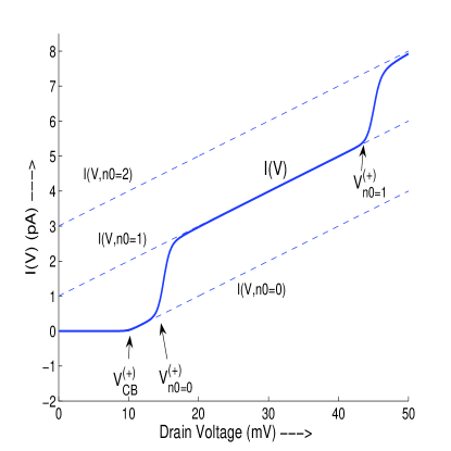
Figure 3: (Color Online) Illustration of Orthodox Model: The orthodox theory parameters define a set of $I(V,n_{0})$ curves, represented by the dashed lines. Generally $n_{0}$ is initially zero. As a voltage is applied, the current follows the $I(V,n_{0}=0)$ curve until $n_{0}$ changes. If $|V_{CB}|<|V_{n_{0}=0}|$, as is the case here, the current will rise linearly out of the zero-conductance region; otherwise, there will be a “jump onset.” For this simulation, $R_{1}=10$ M$\Omega$, $R_{2}=6$ G$\Omega$, $C_{1}=8$ aF, $C_{2}=5.3$ aF, $Q_{0}=0$, and $T=2$ K.

We thus have an intuitive picture of how I-V ($I-V_{D}$) curves are constructed in the orthodox theory. For given system parameters (R, C, etc.) and gate voltage, there is a set of $I(V,n_{0})$ curves for different values of $n_{0}$, as dictated by Eq. (11). The dashed lines in Fig. 3 correspond to three members of such a set. In general, both $n_{0}$ and $I$ are initially zero. As a drain voltage is applied, I(V) remains on the $I(V,n_{0}=0)$ curve until $n_{0}$ changes, at which point I(V) jumps to the $I(V,n_{0}=\pm 1)$ curve. Generalizations of Eqs. (5,6a) from Hanna and Tinkham Han91 allow one to specify the Coulomb Blockade threshold voltages,

$$V_{CB}^{(+)}=C_{1}^{-1}(e/2-n_{0}e+Q_{0}+C_{G}V_{G})$$ (12a)

$$V_{CB}^{(-)}=C_{1}^{-1}(-e/2-n_{0}e+Q_{0}+C_{G}V_{G})\mbox{,}$$ (12b)

and the voltages at which the system transitions from $n_{0}$ to $n_{0}\pm 1$ electrons,

$$V_{n0}^{(+)}=C_{2}^{-1}(e/2+n_{0}e-Q_{0}-C_{G}V_{G})$$ (13a)

$$V_{n0}^{(-)}=C_{2}^{-1}(-e/2+n_{0}e-Q_{0}-C_{G}V_{G})\mbox{.}$$ (13b)

In Eqs. (12,13) the positive superscripts refer to positive onset voltages, and the negative superscripts are similarly defined. In Fig. 3, for example, we can see that the CB threshold voltage is reached (at $10$ mV) before $n_{0}$ increases (at $15$ mV), resulting in a linear onset of the current. If, however, $|V_{n0}^{(\pm)}|$ were smaller than $|V_{CB}^{(\pm)}|$, then there would be a “jump” onset at the zero-conductance region threshold.

Let us now compare the orthodox and Fock space model approaches to transport in the CB regime and apply them within the context of experimental trends.

IV CB Asymmetries: Gate Dependent Rectification

One of the simplest consequences of asymmetric contact coupling is rectification; in other words, a bias direction dependence in the I-V characteristics. To calibrate with experiments, we not only concern ourselves with rectification per-se, but also how it is influenced by a gate. In fact, experiments jpark ; rscott showcase gate dependences of the rectification properties that are arguably more interesting than the rectifications themselves. These experiments (see for example jpark ; rscott ) show the following gate-able features: (i) a gate-dependent shift of conductance peak onsets and (ii) a gate-dependent modulation of the corresponding conductance peak heights. In addition, there is (iii) a prominent exchange in conductance peak asymmetry for gate voltage variations about the charge degeneracy point in the stability diagram rscott . We will argue that much of the relevant physics has to do with the way the molecule accesses various electronic excitations under bias, which would require going beyond our one-orbital model to a multi-orbital system. Charge addition or removal causes jumps in the I-V, while charge redistribution (excitation) leads to closely spaced plateaus that merge onto a linear ramp when summed incoherently. In the rest of the section, we will explain how each CB model (Fock-space and orthodox) successfully captures the gate modulation of the asymmetric I-Vs, as summarized schematically in Figs. 4 and 7.

IV.1 Gate Modulation of current onsets and heights

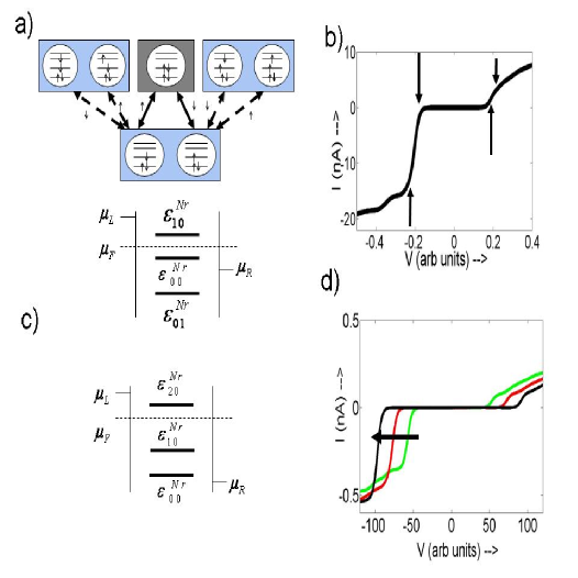
Figure 4: (Color Online) Origin of peak asymmetry and variation with gate voltage. (a) For gate voltages that place the contact Fermi energy $\mu_{F}$ in the $N$ electron blockade region, the levels align such that $\mu_{F}>\epsilon^{Nr}_{00}$. A state transition diagram (b) shows the addition and removal of up (down) spins resulting in transitions $\epsilon^{Nr}_{00}$ (bold double arrow) between ground states of neutral (light orange) and positively charged species (light blue). Also shown in state transition diagram are transitions (dashed double arrow) between various configurations of neutral excited state (deep orange) and positively charged ground state, labeled $\epsilon^{Nr}_{10}$. (c) The resulting G-V shows clear asymmetry in conductance peak height due to there being more ways to add an electron. Increasing gate bias increases the number of excitations available, giving a pronounced peak modulation with gate voltage. The inset shows the corresponding I-V characteristics rbhasko ; jpark ; rscott

The onset of conduction is determined by the offset between the equilibrium Fermi energy and the first accessible transition energy, marked $\epsilon^{Nr}_{00}$ in Fig. 4 (following the nomenclature in section II A). This can be varied by varying the gate voltage, thereby accounting for the variation in conductance gap with gate bias (Fig. 4c). While the current step and corresponding conductance peak are generated by this threshold transition, there follows a quasi-ohmic rise in current leading to a subsequent constant non-zero conductance in the G-V. This feature arises from the sequential access of several closely spaced transport channels under bias, arising from excitations within the $N$ and $N-1$ electron subspaces rbhasko . While net charge addition and removal come at large Coulomb prices, excitations involve charge reorganization within the Fock space that cost much smaller correlation energies.

The presence of multiple orbitals generates several configurations of excited states, creating more accessible transport channels within the bias window. For example, in Fig. 4(a) conduction occurs simultaneously via the $\epsilon^{Nr}_{10}$ and $\epsilon^{Nr}_{00}$ removal channels. $\epsilon^{Nr}_{10}$ corresponds to a transition between the first excited state ‘1’ of the $N$-electron neutral species, and the ground state ‘0’ of the $N-1$ electron cationic species. We show four possible configurations corresponding to the transport channel $\epsilon^{Nr}_{10}$ and the corresponding I-V (Fig. 4b). Increasing the gate bias increases both the threshold for current conduction and the number of such excited state channels accessed by the contacts, thereby altering the height of the corresponding conductance peak with gate bias (Fig. 4c).

The previous paragraph illustrates the origin of gate-modulated current as rationalized by the Fock-space CB model. One can also explain this within the simpler orthodox model, which ignores the identities of the resolved excitations by incoherently summing over them. Under the approximations of contact asymmetry and low temperature, the rate $R^{(j)}_{N\rightarrow{N\pm 1}}$ is linear in the transition energies $\Delta E_{j}^{\pm}$ that increase with drain voltage. With increasing gate bias one needs a larger corresponding drain bias to overcome the zero-conductance regime. At this higher drain voltage the coupling has a greater value and, consequently, the current magnitude is larger. Physically, the drain voltage-dependence of the coupling represents a linear approximation of the excitation spectra. Even though the orthodox model indiscriminately sums the excitations within the $N$ and $N-1$ subspaces, the fact that it captures them at all allows it to qualitatively capture the modulation of current height.

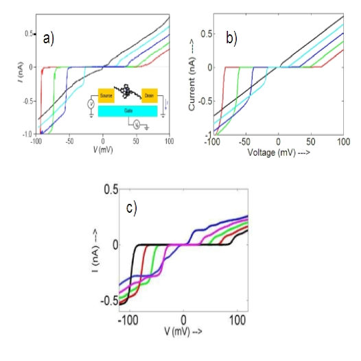
Figure 5: (Color Online) Experiment from J. Park el al. jpark showing gate-rectification properties in the Coulomb Blockade regime: a) Experimental traces, b) Orthodox fit with parameters $C_{1}=0.624$ aF, $C_{2}=0.486$ aF, $C_{G}=0.0708$ aF, $R_{1}=1$ M$\Omega$, $R_{2}=75$ M$\Omega$, $Q_{0}=-0.05e$ and $T=2.2$ K. c) Fit from Fock-space model.

Figs. 5(a) and 6(a) show experimental evidence of gate-modulation of current onsets and heights. Fig. 5(a), from J. Park et al., shows a simple experiment for which the negative bias onset is set by moving from the $N$ to $N-1$ electron subspace, while the positive bias onset starts where the $N$ electron excitation spectrum moves into the bias window. Figs. 5(b,c) show the abilities of both the orthodox model and the Fock-space model to capture the gate-modulated features of the experiment. Fig. 6(a), by Zhitenev et al., is a similar experiment with slightly more complex features. Curves (d-h) show the same negative bias onset as seen in Fig. 5, but as the gate voltage is further decreased, the negative onset changes to a linear onset, representing access to the $N$ electron excitation spectrum. The positive bias shows that decreasing gate voltage brings the $N+1$ level closer to the bias window, and for curves (a-c) the positive bias type consequently becomes a “jump” onset. In spite of these new degrees of freedom that must be captured, the orthodox theory still models very accurately, as seen in Fig. 6(b). It is worth noting that the x-axis in Fig. 6 is $V_{SD}$, rather than $V_{DS}$, which must be accounted for when using Eqs. (9-13) of the orthodox theory. A discussion of the extraction of orthodox parameters from the experimental curves in Figs. 5 and 6 is included in the appendix.

Mathematically, it is straightfoward to understand the dependence of current height on gate voltage within the orthodox theory. Using the experiment of J. Park. et al. (Fig. 5a) as an example, we see that there is a jump onset for negative bias voltages. Therefore, $\left|V_{n0}^{(-)}\right|<\left|V_{CB}^{(-)}\right|$. At $V_{n0}^{(-)}$, the I-V transitions to the $I(V,n0=-1)$ curve, so to find the current height at the onset voltage we can use Eq. (11) for $n_{0}=-1$. Inserting $V_{n0}^{(-)}$ for $V_{D}$, one finds:

$$I(V_{n0}^{-})=-\frac{C_{1}+C_{2}}{R_{2}C_{2}C_{\Sigma}}\left(Q_{0}+e/2+C_{G}V_{G}\right)$$ (14)

Clearly the magnitude of the current at the onset voltage increases with gate voltage (Fig. 5b), matching the experimental result seen in Fig. 5(a).

   

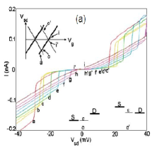
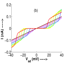
Figure 6: (Color Online) Asymmetric CB results showing (a) experiment zhitenev and (b) orthodox theory with parameters $C_{1}=3.70$ aF, $C_{2}=3.24$ aF, $C_{G}=0.061$ aF, $R_{1}=2$ M$\Omega$, $R_{2}=210$ M$\Omega$, $Q_{0}=0.175e$, and $T=4.2$ K.

The accuracy of the orthodox simulation would imply at the very least that individual excitations do not play an important role in the transport characteristics seen. Because the experimental I-V has a strongly linear dependence on drain voltage seen in Eq. (11), it seems that the experiments may have measured transport through a metallic particle, which has a relatively featureless density of states, as is assumed in the orthodox model.

IV.2 Peak Exchange

Experiments exhibit a characteristic flipping of conductance peak asymmetry around the charge degeneracy point A in the stability diagram (Figs. 7a,b). Figs. 7(e,f) show typical calculated G-Vs in this regime, featuring conductance peak asymmetries with respect to voltage bias, arising due to asymmetric contact couplings ($\gamma_{L}\gg\gamma_{R}$). Within the Fock-space model, this can be explained by enumerating the channels for adding and removing electrons under bias (Figs. 7b,d), with the weaker right contact once again setting the rate limiting step. The dominant transport channel $\epsilon^{Nr}_{00}$ corresponds to electronic transitions between the neutral and cationic ground states rbhasko , states which SCF theories do take into account. In the CB limit, however, there are additional electronic excitations that are accessible with very little Coulomb cost. These states are responsible for the peak asymmetry exchange observed in these experiments, as we will now explain.

The origin of this asymmetry can be understood with a simple model system: in our case, a quantum dot with 8 spin-degenerate levels and $N=4$ electrons in its ground state. When the Fermi energy lies to the immediate right of the charge degeneracy point as shown in Fig. 7(a), only transitions between the $N$ and $N-1$ electron states (4 and 3) are allowed, with the weaker right contact setting the rate-limiting step. For positive bias on the right contact an electron can be removed from the 4-electron to the 3-electron ground state in two ways (Fig. 7b)). For negative bias, however, the electron removed by the left contact can be replenished by the right contact back into the 4-electron ground state, but also into one of many possible excited states $\epsilon^{4r}_{i0}=E^{4}_{i}-E^{3}_{0}$, (i $>$ 0). Since there are more ways to bring the electron back (6 shown here), the conductance is larger for negative bias (Fig. 7e). The situation changes dramatically for a different position of the Fermi energy (Fig. 7c) in the stability diagram lying to the left of the charge degeneracy point A with three electrons at equilibrium. For negative bias the right contact adds an electron from the 3 to the 4-electron ground state, while for negative bias it returns it to the $j^{th}$ 3-electron excited state through transitions $\epsilon^{4r}_{0j}=E^{4}_{0}-E^{3}_{j}$. There now are more ways to remove than add charge (Fig. 7d), so the asymmetry flips (Fig. 7f).

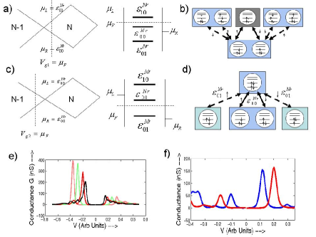
Figure 7: (Color Online) Origin of exchange in asymmetry of conductance peaks: (a), (b) Schematic of vicinity of charge degeneracy point A in Coulomb diamond. Also shown are the corresponding energy diagrams at threshold. Notice a different set of threshold transport channels between (a) and (b). (c) and (d) State transition diagrams illustrating the different excitation spectra accessed on either side of the charge degeneracy point A. (e) and (f) G-V plots for scenarios (a) and (b) Notice the clear peak-exchange as a result of accessing a different excitation spectra in either case.

Analogous to the Fock-space model, the orthodox model also captures gate-dependent peak exchange, in spite of its approximate treatment of excitations. The origin of the asymmetry is once again transitions between the $N$ to $N-1$ electron regimes. In Fig. 3, we can see that such a change results in a jump onset that has a much higher conductance value than a linear onset. Moving from the $I(V,n0)$ curve to the $I(V,n0-1)$ curve, therefore, essentially captures the excitations of the $N-1$ electron spectrum that are pivotal to the argument in the preceding paragraph. The fact that the conductance peak switches across zero bias only means that the zero-bias state of the system changes from $N$ to $N-1$ electrons, which the orthodox method clearly captures.

Peak exchange has been reported experimentally rscott , as seen in Fig. 8(a). Fig. 8(b) shows an orthodox simulation of the experiment. One can see close qualitative as well as quantitative agreement between the experimental data and the theoretical simulation. The conductance peaks have similar magnitudes, and the exchange of the peak asymmetry occurs at $-3.75$ $V$ in both graphs. The evident validity of the orthodox theory in this case demonstrates its ability to capture excitation features, as long as the features can be linearly approximated.

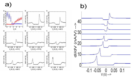
Figure 8: (Color Online) (a) Experimental trace demonstrating peak asymmetry exchange rscott . Compare with Fock-space model results in Fig. 7(e,f). (b) Orthodox simulation reproducing peak exchange observed in the experiments. The parameters are: $R_{1}=35$ M$\Omega$, $R_{2}=350$ M$\Omega$, $C_{1}=0.673$ aF, $C_{2}=0.612$ aF, $C_{G}=0.0135$ aF, $Q_{0}=-0.18e$, and $T=4.2$ K.

V Limitations of the Orthodox Model

In the previous sections, we saw that the orthodox model has been fairly successful in reproducing the three key trends in asymmetric CB transport; namely, (i) rectification, (ii) gate-modulation of rectification and (iii) exchange of rectification. The agreement between experiment and theory are quantitatively quite close, indicating that the Fock-space model’s handling of well-resolved excitations is perhaps an overkill, especially considering its substantially greater computational complexity. It is tempting to conclude that molecules with redox-active centers only exhibit incoherent sums of excitations that do not manifest well-resolved features. In this section, we point out examples where the discrete excitation spectrum can indeed play a noticeable role in molecular transport experiments, making an orthodox theoretical treatment quite inadequate.

Molecules are unique in that they can potentially exhibit both charge and size quantization rbhaskob . Charge quantization is enforced by $U>\Gamma$, which amounts to a large contact resistance compared to the resistance quantum (the correspondence arises by relating the broadening $\Gamma$ to an RC time-constant through the uncertainty principle, using the capacitance $C$ to set the single-electron charging energy $U$). At the same time, the small sizes of molecules make their spectra discrete. While transport examples showcasing discrete molecular signatures are relatively rare, they are pretty commonplace in the literature of inorganic quantum dots or ‘artificial molecules’ rbanin . Part of the reason is the lower broadening in these dots, both from the contact as well as incoherent scattering (which is larger in organic molecules owing to their conformational flexibility). Recently, a novel negative differential resistance (NDR) has been reported in inorganic double quantum dots tar , that has been explained via the formation of an excited triplet state tar ; rbhasko2 . Other quantum dot experiments routinely show Coulomb diamonds with very well resolvable excitation lines sampaz such as due to cotunneling cotunel and Kondo correlations kondo .

Well resolved excitation lines in the conductance spectra manifest as varying plateaus in the I-V characteristics. Consider the low bias ($V_{D}<500$ mV) I-V characteristics of the plot from J-O. Lee et al. rdekker , seen in Fig. 9. A striking feature is the existence of a plateau at onset followed by several other plateaus, sometimes even merging into a quasi ohmic rise as a result of several unresolvable plateaus. This feature, observed in multiple experiments from other experimental groups, can be easily explained within the Fock-space model by keeping track of individual molecular excitations. For example, it is well known that the gap between ground and first excited states, involving charge addition or removal, is greater than the gap between subsequent excitations involving charge reorganization. In such a case it is clearly seen that a brief plateau occurs at threshold that persists until the first excitation is been accessed, as discussed in detail in rbhasko .

This leads to an important point. Normally small plateaus (few tens of mV) are naturally associated with vibronic modes whose energy scales lie in that range. Coulomb interactions are usually assumed to be larger in energy, because the energy to add or remove an electron is much larger. However, the correlation energy to reorganize charges could actually be very small, are therefore quite capable of explaining a range of plateau widths seen experimentally, as our calculations show.

The orthodox theory, on the other hand, cannot even qualitatively match the experimental data in Fig. 9, owing to its inability to incorporate size quantization effects and the associated discrete spectra. From Eq. 11, it is clear that outside of the zero-conductance region and excluding jumps due to changes in $n_{0}$, conductance values in orthodox theory must remain constant, with a value of $R_{1}/R_{2}C_{\Sigma}$. The orthodox theory can capture a plateau, and it can also capture a linear rise, but it does not seem to capture both in the same I-V curve. Fig. 9(c) shows the best attempt at modeling the experimental data in Fig. 9(a) within orthodox theory; the plateau followed by a linear rise seems hard to duplicate.

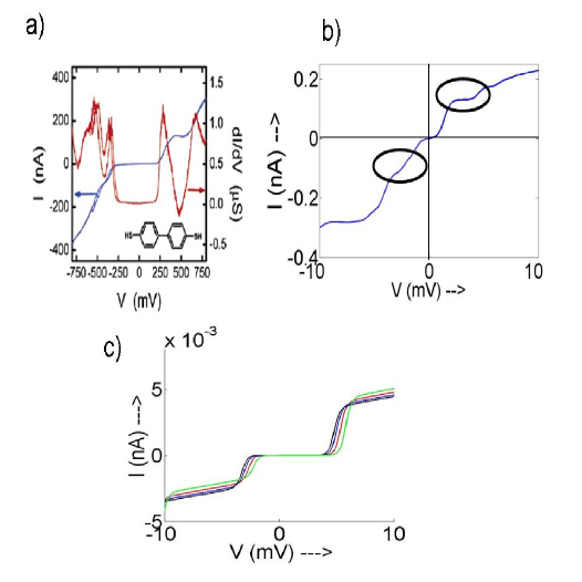
Figure 9: (Color Online) Limitation of Orthodox Model: a) Experimental trace rdekker showing fine structure. b) The fine structure in I-V’s, result from keeping track of excitations explicitly within the Fock-space CB model. c) An orthodox calculation merely maintains the same slope between charge addition jumps, thus may not reproduce any fine structure.

A second limitation of the orthodox model comes in its treatment of gate voltage. Even though it effectively modeled the data in Figs. 5, 6 and 8, there again exist experimental features that the orthodox theory cannot even qualitatively model. Looking at Eqs. (12) and (13) one can see that a change in gate voltage causes a translation in the Coulomb Blockade threshold voltages; a similar effect, albeit in the opposite direction, is seen for the voltage limits at which $n_{0}$ changes. Fig. 10 shows how an orthodox I-V curve changes with gate voltage for the four possible onset combinations - which come from having linear or jump onsets at positive and negative bias. The scaling of the conductance gap in Figs. 10(a,b) successfully explained the experiments in Figs. 5 and 8. However, for experiments with symmetric onsets (Figs. 10c,d), one can see that the orthodox theory predicts an overall translation in the I-V curve with gate voltage. One would think that changing the gate voltage would only shift the conducting level closer to or further from the bias window, thereby narrowing or widening the I-V curve, respectively. Indeed, experimental evidence demonstrates such narrowing rralph2 , and the Fock-space model captures that quite easily. The orthodox theory was unable to match this experimental trend even qualitatively.

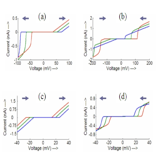
Figure 10: (Color Online) Gate-voltage dependence of I-V curves in the orthodox theory. Blue arrows indicate the direction of movement of the onset voltages with increasing gate voltage. The four plots correspond to the four possible onset combinations: (a) a jump onset at negative bias and a linear onset at positive bias, for which the I-V conductance gap widens with increasing gate voltage; (b) a linear onset then a jump onset, with the gap narrowing around zero-bias; (c) two linear onsets, which corresponds to a translation of the I-V curve, and (d) two jump onsets, which correspond to a translation in the opposite direction of (c).

VI Discussions

It may seem that the proper treatment of well-resolved excitations is rather academic with respect to molecular experiments. However, we believe that there can be more important experimental features that need a proper quantitative theory as transport spectroscopy of molecules under becomes feasible ucla . In fact, a possible explanation for molecular NDRs tour ; kiehl could necessitate keeping track of excitations in a donor-acceptor molecular system rbhasko2 ; in particular, the notably different lifetimes of ground and excited states, analogous to issues relevant to the double quantum dot literature. Small molecules could function as tunable quantum dots with high single-electron charging energies. Molecular quantum dots coupled to transistor channels can be important for the detection, characterization and manipulation of individual spin qubits ucla , the transistor conductance providing a way to achieve electronic read-out rabi . The large charging energies could allow redox-active molecules to operate as storage centers for memory misra . Finally, rectification is important to avoid parasitic pathways in cross-bar logic based architectures stan .

The accurate treatment of well-resolved excitations is crucial to molecular operation in this scattering regime. But the price paid for this accuracy is the loss of simplicity associated with orthodox theory. Instead, we will need a major improvement in computational algorithms to handle the exponential scaling of the many-body Fock space, such as partial configuration interaction (CI) with frontier orbitals coupled to the standard master equations. Major challenges involve the proper inclusion of the contact boundary conditions, and doing justice to broadening rWacker . Also, one could incoherently sum selected excitations and resolve the relevant ones, if we have some prior idea which ones could be important. Spin unrestricted approaches may capture some of the salient effects, although they are unlikely to capture the current heights (which depend on difficult parameter-independent combinatorial arguments), and even more significantly, the number of current plateaus (since an energy-independent one-electron potential does not generate enough poles). Needless to say, there is enormous room for theoretical activity and device potential in this domain.

It is worth emphasizing that the wide success and popularity of the SCF-NEGF approach often leads researchers to automatically assume that the method will work in the CB regime revers ; rpal . The NEGF method is indeed prolific in its flexibility to incorporate contact microstructure, molecular chemistry, broadening, intereference and electrostatic details. However, the method, as widely implemented, is fundamentally limited by the need to work with a one-electron potential, at best incorporating many-body effects as corrections to this potential. While this may be sufficient to capture equilibrium properties like total energy, transport measurements can potentially probe the rich excitation spectra that are hard to incorporate readily into the average electronic potential, even parametrically. For a typical self-energy, there simply are not enough poles in the one-electron Green’s function to do justice to the many more many-electron transitions characterizing transport, not to mention the complications of the full counting statistics in Fock space under non-equilibrium that show up as effective interaction-independent degeneracies of the open-shell levels.

In this paper, we have discussed contact asymmetry as a paradigm to delve into various experimental features, outlining the qualitative difference and cross-over between the weakly correlated SCF and the strongly correlated CB regimes. An understanding of the asymmetry was provided using a basic model, and then extended to conjugated molecular systems. Novel experimental-trends were identified in the CB-regime of transport. Two different approaches, the Fock-space CB and the orthodox CB, were discussed in detail. While a simpler orthodox approach captures the salient asymmetric effects, the Fock-space approach may be essential in examples where the interplay between specific excitations governs the principle operating physics and possibly also interesting device applications envisaged.

VII Acknowledgments

We would like to thank S. Datta, L. Harriott, G. Scott and H-W. Jiang for useful discussions. This project was supported by the DARPA-AFOSR grant.

VIII Appendix I: Extracting parameters for orthodox model

The low temperature, strong contact asymmetry approximation to the orthodox theory, as introduced in section III, is most useful because it simplifies the process of simulating experimental data. Whereas the general orthodox formalism requires best-fit computational techniques, Eqs. (11-12) allow for a straightforward analytic calculation of the system circuit parameters. Consider Fig. (5) as an example of data to be simulated with the orthodox theory. To start, consider the $V_{G}=-0.85V$ I-V curve (light blue). We have a linear onset at approximately $19$ $mV$, and a “jump” onset at, say, $-24$ $mV$. Plugging these values into Eqs. (11a) and (12b), respectively, and solving finds:

$$C_{1}(19mV)=C_{2}(24mV)\mbox{, and}$$ (15)

$$C_{1}=\frac{e+2Q_{0}+2C_{G}V_{G}}{2(19mV)}\mbox{.}$$ (16)

Consideration of a second I-V curve in the data gives us further information; here we will use the $V_{G}=-0.55V$ (green) curve, which has a positive onset voltage of approximately $53$ mV. After plugging the correct onset and gate voltage values into Eq. (11a) for both I-V curves considered, one can solve for a new, independent equation:

$$C_{1}=\frac{\Delta V_{G}}{(53-19)mV}C_{G}=8.82C_{G}$$ (17)

We now have three equations and four unknowns ($C_{1}$, $C_{2}$, $C_{G}$, and $Q_{0}$). There are now two approaches one can take. The first, which was applied in the simulation shown in Fig. 4(b), is to simply take a small, reasonable value of $Q_{0}$, such as $-0.05e$, and solve the remaining equations for the other variables. However, this will not always work, for a reason that is somewhat subtle. It is important to note in Fig. 4(a) that not only does the $V_{G}=-0.85V$ I-V curve have a linear onset at $19$ $mV$, but it also does not have a jump onset at positive bias until at least $100$ $mV$. Setting Eq. (12a) greater than $100$ $mV$ provides a fourth restriction. Indeed, for the experiment in 4(a) this is trivially satisfied; Fig. 6, on the other hand, is an example of data for which such a fourth equation is necessary for a successful simulation.

A final parameter one can obtain is $R_{2}$. From Eq. (7) we know that the conductances of the linear portions of orthodox curves have the value $C_{1}/R_{2}C_{\Sigma}$. Having already calculated all of the capacitance values it is thus straightforward to find the slope of the experimental I-V curve and find $R_{2}$. $R_{1}$ cannot be found so easily, but its relative unimportance in the regime of contact asymmetry means that a simple estimate of $R_{1}\sim R_{2}/100$ will usually suffice.

References

- (1) A. Aviram and M. A. Ratner, Chem. Phys. Lett. 29, 277 (1974).
- (2) J. Reichert, R. Ochs, D. Beckmann, H. B. Weber, M. Mayor, and H. v. L’́ohneysen Phys. Rev. Lett. 88, 176804 (2002).
- (3) J. Park, A. N. Pasupathy, J. I. Goldsmith, C. Chang, Y. Yaish, J. R. Petta, M. Rinkovski, J. P. Sethna, H. D. Abruna, P. L. McEuen, and D. C. Ralph , Nature 417, 722 (2002).
- (4) Gavin D. Scott, Kelly S. Chichak, Andrea J. Peters, Stuart J. Cantrill, J. Fraser Stoddart and H. W. Jiang cond-mat/0405345, and Gavin D. Scott, Kelly S. Chichak, Andrea J. Peters, Stuart J. Cantrill, J. Fraser Stoddart and H. W. Jiang Phys. Rev. B 74, 113404 (2006).
- (5) F. Zahid et al., Phys. Rev. B 24,245317 (2004).
- (6) M. M. Deshmukh et al., Phys. Rev. B 65, 073301 (2002).
- (7) S. Datta, ‘Quantum Transport: Atom to Transistor’, Cambridge University Press, (2005).
- (8) M. Koentopp, C Chang, K. Burke, and R. Car, cond-mat/0703359, and references therein.
- (9) P. S. Damle, A. W. Ghosh and S. Datta, Chem. Phys. 281, 171 (2002).
- (10) B. Muralidharan, A. W. Ghosh and S. Datta Phys. Rev. B 73, 155410 (2006).
- (11) B. Muralidharan, A. W. Ghosh and S. Datta, J. Mol. Sim. 32, 751 (2006).
- (12) B. Muralidharan, A. W. Ghosh, S. K. Pati and S. Datta, IEEE Trans. Nanotech, (2007) (in press).
- (13) M. Koentopp, F. Evers, and K. Burke, Phys. Rev. B (R) 73 121403 (2006).
- (14) J. J. Palacios, Phys. Rev. B 72, 125424 (2005).
- (15) C. Toher, A. Fillipetti, S. Sanvito and K. Burke, Phys. Rev. Lett 95, 146402 (2005).
- (16) P. Pals and A. MacKinnon, J. Phys.: Condens. Matter. 8, 5401 (1996).
- (17) M. H. Hettler, W. Wenzel, M. R. Wajewijs, and H. Schoeller, Phys. Rev. Lett. 90, 076805 (2003).
- (18) B. Muralidharan and S. Datta, Phys. Rev. B (2007) (in press).
- (19) L. Siddiqui, A. W. Ghosh and S. Datta, Phys. Rev. B (accepted).
- (20) F. Elste and C. Timm, Phys. Rev. B 71, 155403 (2005).
- (21) J. N. Pedersen and A. Wacker, Phys. Rev. B, 72, 195330, (2005).
- (22) K. M. Indlekofer, J. Knoch and J. Appenzeller, cond-mat/0609025.
- (23) G. Klimeck, G. L. Chen and S. Datta, Phys. Rev. B, 50, 2316, (1994).
- (24) F.P.A.M. Bakkers, Z. Hans, A. Zunger, A. Franceschetti, L.P. Kouwenhoven, L. Gurevich, and D. Vanmaekelbergh, Nano. lett. 1, 551, (2001).
- (25) S. Braig and P. W. Brouwer, Phys. Rev. B 71, 195324 (2005).
- (26) E. Bonet et al., Phys. Rev. B 65, 045317 (2002); C. W. J. Beenakker, Phys. Rev. B 44, 1646 (1991).
- (27) V. V. Shorokhov, P. Johansson, and E. S. Soldatov, J. Appl. Phys. 91, 3049 (2002).
- (28) ‘Single Charge Tunneling’, Ed. H. Grabert, and M. H. Devoret, NATO ASI series 294, Plenum Press, New York, 1992.
- (29) A. W. Ghosh (unpublished). The main role of dephasing is to add an exclusion principle term in each up or downconversion rate. Dephasing tends to localize the electrons and thereby introduces the exclusion term.
- (30) A. E. Hanna and M. Tinkham, Phys. Rev. B 44, 5919 (1991).
- (31) H. Zhang, Y. Yasutake, Y. Shichibu, T. Teranishi, and Y. Majima, Phys. Rev. B 72, 205441 (2005).
- (32) N. B. Zhitenev, H. Meng, and Z. Bao, Phys. Rev. Lett., 88, 226801 (2002).
- (33) U. Banin, Y. Cao, D. Katz, and O. Millo, Nature, 400, 542, (1999).
- (34) K. Ono, D. G. Austing, Y. Tokura, and S. Tarucha, Science 297, 1313 (2002).
- (35) see for example: S. Sapmaz, P. Jarillo-Herrero, J. Kong, C. Dekker, L. P. Kouwenhoven, and H. S. van der Zant, Phys. Rev. B,71 153402 (2005) and references therein.
- (36) S. DeFranceschi, S. Sasaki, J. M. Elzerman, W. G. Van Der Wiel, S. Tarucha, and L. P. Kouwenhoven, Phys. Rev. Lett, 86, 878 , (2001).
- (37) D. Goldhaber-Gordon, H. Shtrikman, D. Mahalu, D. Abusch-Magder, U. Meirav, and M. A. Kastner, Nature, 391, 156 (1998).
- (38) J-O. Lee, G. Lientschnig, F. Wiertz, M. Struijk, R. A. J. Janssen, R. Egberink, D. N. Reinhoudt, P. Hadley, and C. Dekker, Nano Lett. 3, 113 (2003).
- (39) M. Xiao, I. Martin, E. Yablonovitch and H. W. Jiang, Nature 430, 435 (2004).
- (40) J. Chen, M. A. Reed, A. M. Rawlett. J. M. Tour, Science, 286, 1550 (1999).
- (41) R. A. Kiehl, J. D. Le, P. Candra, R. C. Hoye, and T. R. Hoye, Appl. Phys. Lett., 88, 172102, (2006).
- (42) F. H. L. Koppens, C. Buizert, K. J. Tielrooij, I. T. Vink, K. C. Nowack, T. Meunier, L. P. Kouwenhoven and L. M. K. Vandersypen, Nature, 442, 776, (2006).
- (43) Q. Li, S. Surthi, G. Mathur, S. Gowda, Q. Zhao, T. A. Sorensen, R. C. Tenent, K. Muthukumaran, J. S. Lindsey and V. Misra, Appl. Phys. Lett. 85, 1829 (2004).
- (44) M. Stan, P. Franzon, S. Goldstein, J. Lach, M. Ziegler, Proc. IEEE 91, 1940 (2003).
- (45) M. Elbing, R. Ochs, M. Koentopp, M. Fischer, C. von Hanish, F. Weigend, F. Evers, H. B. Weber, and M. Mayor, Proc. Natl. Acad. Sci, 102, 8815, (2005); J. J. Palacios, Phys. Rev. B 72, 125424 (2005).