Effects of the low frequencies of noise on On–Off intermittency

Abstract

A bifurcating system subject to multiplicative noise can exhibit on–off intermittency close to the instability threshold. For a canonical system, we discuss the dependence of this intermittency on the Power Spectrum Density (PSD) of the noise. Our study is based on the calculation of the Probability Density Function (PDF) of the unstable variable. We derive analytical results for some particular types of noises and interpret them in the framework of on-off intermittency. Besides, we perform a cumulant expansion VanKampen1 for a random noise with arbitrary power spectrum density and show that the intermittent regime is controlled by the ratio between the departure from the threshold and the value of the PSD of the noise at zero frequency. Our results are in agreement with numerical simulations performed with two types of random perturbations: colored Gaussian noise and deterministic fluctuations of a chaotic variable. Extensions of this study to another, more complex, system are presented and the underlying mechanisms are discussed.

I Introduction

Most patterns observed in nature are created by instabilities that occur in an uncontrolled noisy environment: Convection in the atmospheric layers and in the mantle are subject to inhomogeneous and fluctuating heat flux; sand dunes are formed under winds with fluctuating directions and strengths. The fluctuations usually affect the control parameters driving the instabilities, such as the Rayleigh number which is proportional to the imposed temperature gradient in natural convection. Thus, these fluctuations act multiplicatively on the unstable modes. In the same spirit, the evolution of global quantities, averaged under small turbulent scales, can be represented by a nonlinear equation with fluctuating global transport coefficients that reflect the small scales complexity. For instance, it has been shown that the temporal evolution of the total heat flux in rotating convection can be described by a non–linear equation with a multiplicative noise Neufeld . The dynamo instability that describes the growth of the magnetic field of the stars and some planets because of the motion of conducting fluids in their cores, is usually analyzed in similar terms: the magnetic field is expected to grow at large scale, forced by a turbulent flow. Here again, the parameters controlling the growth rate of the field are fluctuating Sweet .

Since the theoretical predictions of Stratonovich Strato , and the experimental works of Kawaboto, Kabashima and Tsuchiya Kawakubo , it is well known that a multiplicative noise may modify an instability process. These early investigations motivated numerous studies on the effect of multiplicative noise on an instability threshold. It can be shown in many cases that the noise induces a drift for the instability threshold (see for instance Schenzle ; Horm ; Lucke1 ; Kirone1 ; Sebetmoi ). Besides, T. Yamada et al Yamada have shown that multiplicative noise can lead to a new type of intermittency, called On–Off Intermittency, in which quiet and laminar (off) phases randomly follow bursting (on) phases. This intermittency has been identified in experiments in various fields: electronics, electro-hydrodynamic convection in nematics, gas discharge plasmas and spin-wave instabilities Hammer .

Most of the theoretical works considered only the effects of a delta–correlated Gaussian white noise or an Ornstein–Uhlenbeck noise with an exponentially decaying correlation function (see for instance the discussion in Horm ). However, with these types of noises that have at most one characteristic time scale, it is difficult to identify which part of the Power Spectrum Density (PSD) of the random forcing really affects the dynamics. On the contrary, the noise in natural environment and also in experimental situations is far from being a white random process. Therefore, we believe that the influence of the noise PSD on an on-off intermittent dynamics deserves to be investigated more precisely.

To motivate further reading of this article, we show in fig.1 the temporal traces of an unstable variable subject to two different multiplicative noises. Both noises have the same standard deviation but different power density spectra. More precisely, in fig.1a, the PSD of the noise has a higher value at zero frequency than in fig.1b. It is clear that the intermittent regime is suppressed if the low frequencies of the noise are reduced even if the standard deviation of the noise is kept constant. To understand this fact, we study in Section $2$ a canonical system and calculate the PDF of the dynamical variable with different methods: exact results for some special types of noises and a perturbative expansion valid for a small noise amplitude. In Section $3$, we compare the predictions of this expansion with numerical simulations. We also study the relation between the low frequencies of the noise PSD and the statistics of the duration of the laminar phases in the intermittent regime (Section $4$). In Section $5$, we present numerical simulations of a bifurcating system of second order in time. We finally give a physical explanation for the relevance of the noise spectrum at zero frequency for on-off intermittency (Section $6$).

Some of the results of this article were published in our letter nous . We give here details on the derivation of these results (Section $2$ and $3$). Besides new systems are investigated (Section $2.3$ and $5$) and a new aspect of the phenomenon is highlighted (Section $4$).

II Analytical predictions

II.1 Case of a Gaussian white noise

We consider the simple system proposed in Yamada to describe on–off intermittency :

$$\dot{X}=(a+\zeta(t))X-X^{3}\,,$$ (1)

where $\zeta$ is a random process with zero mean. This equation describes the evolution of a variable $X$ with instantaneous departure from onset $a+\zeta(t)$ and cubic nonlinearity. Without noise ($\zeta=0$), equation (1) has the fixed points : $X=0$ and $X=\pm\sqrt{a}$ for $a>0$. The former one is stable for negative $a$ and the latter are stable for positive $a$.

Let $\zeta(t)$ be a Gaussian white noise with $\langle\zeta(t)\zeta(t^{\prime})\rangle_{s}=D\delta(t-t^{\prime})$ where $\langle\rangle_{s}$ is the average on the realizations of the noise. The Langevin equation (1) is interpreted as a Stratonovich equation. The stationary Probability Density Function of $X$ can be calculated from the Fokker–Planck equation Schenzle and is given by

$$P(X)=C|X|^{\frac{2a}{D}-1}e^{-\frac{X^{2}}{D}}\,,$$ (2)

for $a>0$; $P(X)=\delta(X)$ if $a\leq 0$. Here, $C$ is a normalization constant.

Several features can be noticed. For positive $a$, there are two different behaviors. When $2a>D$, the most probable values are $X_{mp}=\pm\sqrt{a-D/2}\,$ but when $2a\leq D$ the most probable values vanish and $P(X)$ diverges as $X\rightarrow 0$. For a small departure from threshold, i.e., $2a/D\ll 1$, $P(X)$ is dominated by a decreasing power law over a large range of $X$ and all moments of $X$ grow linearly with $a$. Indeed, equation (2) implies that $\langle X^{2n}\rangle=D^{n}\Pi_{j=0}^{n-1}(a/D+j)$ which leads to $\langle X^{2n}\rangle\simeq aD^{n-1}(n-1)!$ when $2a/D$ is small.

As pointed out in Yamada , the form of the PDF for small $X$ is related to the on–off intermittent character of the variable $X$ : The occurrence of laminar phases are responsible for the divergence of the PDF at $X=0$.

II.2 Expansion for a colored noise

White noise, with all frequencies having the same weight, does not allow to discriminate which frequencies play a role in the occurrence of on-off intermittency. However, as it clearly appears in fig.1, two non-white noises with the same standard deviation but different spectral densities at zero frequency, lead to dynamics that are qualitatively different. Indeed, if the value of the noise PSD at zero frequency is reduced, the laminar phases around zero, that characterize on–off intermittency, can even be suppressed.

To analyze quantitatively this phenomenon, we apply the cumulant expansion to equation (1). The resulting equation for the PDF of $X$ is of the Fokker-Planck type and, in the case under study, is given by

$$\partial_{t}P=\partial_{x}\left(\left((1+\frac{S-M}{a})X^{3}-(a+S)X\right)P\right)+\partial_{x^{2}}\left(\left(SX^{2}+\frac{M-S}{a}X^{4}\right)P\right)\,.$$ (3)

The derivation of this equation is presented in Appendix. The two coefficients that appear in this effective Fokker-Planck equation depend on the noise as follows

$$S = \int_{0}^{\infty}\langle\zeta(0)\zeta(\tau)\rangle_{s}d\tau\,,$$

$$M = \int_{0}^{\infty}\langle\zeta(0)\zeta(\tau)\rangle_{s}e^{-2a\tau}d\tau\,.$$ (4)

The parameter $S$ is given by the integral of the autocorrelation function of the noise and is equal to half of the PSD of the noise at zero frequency by virtue of the Wiener–Khintchine theorem. The parameter $M$ is also related to the integral of the autocorrelation function but with a reduced weight of its long-time values. The steady state solution of equation (3) for the generic case $S\neq 0$ and $S\neq M$ is given by

$$P(X)=C|X|^{\frac{a}{S}-1}|1+\frac{(M-S)X^{2}}{S\,a}|^{-(1+\frac{a\,M}{2\,S\,(M-S)})}\,,$$ (5)

where $C$ is a normalization constant. Note that this expansion is valid when the product of the time correlation of the noise with its amplitude is small VanKampen1 ; VanKampen2 .

The behavior of the PDF for small $X$ is a power law with exponent $a/S-1$. Consequently, the criterion for on-off intermittency, in the sense that the PDF of the variable diverges for small $X$, is

$$S>a\,.$$ (6)

In other words, the variable is on-off intermittent when the value of the noise spectrum at zero frequency is greater than twice the departure from onset.

We also notice from the power law form of the PDF that all the moments $<X^{2n}>$ grow linearly with the departure from onset $a$, in the limit of small $a$. As in the case of a Gaussian white noise, this behavior is related to the form of the PDF in the vicinity of the unstable fixed point and thus to the occurrence of on-off intermittency.

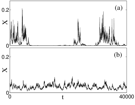
Figure 1: Temporal traces of the dynamical variable $X(t)$ solution of equation (1) with a noise of autocorrelation function given by (14). In both cases, $a=0.00125$, $\alpha^{2}=0.005$. In figure (a), $\eta=\Omega=0.25$ i.e., $a/S=0.3927$; in figure (b), $\eta=\Omega=2.5$ i.e., $a/S=3.9270$.

II.3 An exactly solvable case: the dichotomous Poisson process

It is also possible to calculate the PDF of $X$, solution of equation (1), in the case where the noise is a dichotomous Poisson process. This problem was studied in bruitdicho . We sum it up here and then discuss the consequences on the on-off intermittent regime.

The noise has only two possible values $\pm\Delta$ and during a time $dt$ switches from one value to the other with a probability $\lambda dt$. We thus obtain

$$<\zeta(t)\zeta(0)>_{s}=\Delta^{2}e^{-2\lambda t}\,.$$ (7)

Let $P_{+}(x,t)$ and $P_{-}(x,t)$ be the probabilities for the variable $X$ to attain the value $x$ at time $t$ when the noise is $\Delta$ and $-\Delta$, respectively. These probabilities follow the equations

$$\frac{\partial P_{+}}{\partial t}=-\frac{\partial}{\partial x}\left(((a+\Delta)x-x^{3})\,P_{+}\right)-\lambda(P_{+}-P_{-})\,,$$

$$\frac{\partial P_{-}}{\partial t}=-\frac{\partial}{\partial x}\left(((a-\Delta)x-x^{3})\,P_{-}\right)-\lambda(P_{-}-P_{+})\,.$$ (8)

We consider the case where $a$ is positive so that the fixed point $X=0$ is unstable. For intermittency to be possible, it is necessary that $\Delta>a$ so that the effective growth rate $a+\zeta(t)$ can be negative. In that case, the stationary PDF of $X$ is given by

$$P(X) = P_{+}(X)+P_{-}(X)$$ (9)

$$= C|X|^{\frac{2a\lambda}{\Delta^{2}-a^{2}}-1}|X^{2}-(a+\Delta)|^{\frac{\lambda}{2(a+\Delta)}-1}$$

$$\times|X^{2}+\Delta-a|^{-\frac{\lambda}{2(\Delta-a)}-1}\,,$$

where $C$ is a normalization constant. The PDF of $X$ diverges at small $X$ and therefore $X$ is on-off intermittent if

$$\frac{2a\lambda}{\Delta^{2}-a^{2}}<1\,.$$ (10)

From equation (7) we calculate the parameter $S$ :

$$S=\int_{0}^{\infty}<\zeta(t)\zeta(0)>_{s}dt=\Delta^{2}/(2\lambda)\,,$$ (11)

and write the criteria for on-off intermittency as

$$S\geq\frac{a}{1-\frac{a^{2}}{\Delta^{2}}}\,.$$ (12)

We emphasize that this result is valid for any noise amplitude and correlation time as long as $\Delta>a>0$. When the product of $\Delta^{2}$ with the time correlation $\lambda^{-1}$ of the noise is small, we have $S\ll 1$ and the criterion (6) is recovered. At higher noise amplitudes, we have an explicit expression for the onset of on-off intermittency. Here again, if the parameter $S$ is lowered and the noise standard deviation $\Delta^{2}$ is fixed, on-off intermittency disappears.

III Numerical studies

III.1 Stochastic colored noise

We verify numerically the predicted expression for the PDF, given in equation (5). To wit, we use a colored noise with two characteristic frequencies, $\Omega$ and $\eta$. This noise is generated from the following dynamics Sawford :

$$\dot{A} = -4\pi\eta A-4\pi^{2}(\Omega^{2}+\eta^{2})\zeta+(4\pi)^{3/2}\sqrt{\eta(\Omega^{2}+\eta^{2})/2}\alpha\xi\,,$$

$$\dot{\zeta} = A\,,$$ (13)

where $\xi$ is a Gaussian white noise with $\langle\xi(t)\,\xi(t^{\prime})\rangle_{s}=\delta(t-t^{\prime})$. This equation leads to the following autocorrelation function

$$\langle\zeta(t)\,\zeta(t+\tau)\rangle_{s}=\,\alpha^{2}\exp(-2\pi\eta|\tau|)\left(\cos(2\pi\Omega\tau)+\frac{\eta}{\Omega}\sin(2\pi\Omega|\tau|)\right)\,,\,\,\,\,\,\,\,$$ (14)

where $\alpha^{2}$ is the noise variance and $t_{c}=(2\pi\eta)^{-1}$ is its correlation time. In this case, we obtain correc

$$S = \alpha^{2}\eta/\left[\pi(\eta^{2}+\Omega^{2})\right]\,,$$

$$M = \alpha^{2}(\eta+a/(2\,\pi))/\left[\pi\left((\eta+a/\pi)^{2}+\Omega^{2}\right)\right]\,.$$ (15)

Therefore by varying $\eta$ and $\Omega$, we can tune independently $a/S$ and $\alpha(2\pi\eta)^{-1}$. The Gaussian white noise is recovered in the limit $\eta\rightarrow{\infty}$ with $\alpha^{2}/\eta=D$. The equations (1) and (13) are solved numerically using a fourth-order Runge-Kutta scheme and an Euler implicit method, respectively. Note from equation (1) that $X$ conserves its sign throughout its evolution. In the following, we consider only positive initial values for $X(t=0)$ without lack of generality.

In figure 1, we plot some temporal traces of $X$. Both curves were obtained for the same values of the noise variance $\alpha^{2}$ and departure from threshold $a$. In fig.1a, we have taken $S>a$; in fig.1b, the chosen value of $S$ is ten times smaller so that the ratio $a/S$ becomes larger than unity. In the latter case, intermittency is clearly suppressed, illustrating the fact that no intermittency occurs when the PDF $P(X)$ does not diverge at $X=0$.

In figure 2, we show that the two PDFs corresponding to the temporal traces of figures 1a and 1b are very well described by equation (5). We remark that for small values of $X$, the PDF behaves as a negative power law when $a/S<1$, as expected in the intermittent regime.

In figure 3, the intermittent domain and the non–intermittent domain are delimited in the ($S,a$)–plane. Intermittency disappears when the most probable value, $X_{max}$, becomes non-zero. The behavior of $X_{max}$ as a function of $a$ for $S=0.27$ is shown in the inset of fig.3. For noises with different spectrum, we increase $a$ and determine when on-off intermittency disappears. We observe that the line $S=a$ does indeed separate the two regimes. Note that the expansion leading to equation (6) is valid when $\alpha\tau_{c}\ll 1$, this condition is fulfilled in the simulations we present.

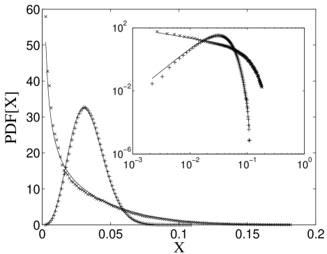
Figure 2: PDF of the solutions of equation (1) for the colored noise given by (14) . The symbols $(\times)$ and $(+)$ correspond, respectively, to the parameters used in figures 1a and 1b. The full lines are the corresponding theoretical approximations given by (5). The inset emphasizes the good agreement of the predicted power law in log–log axes.

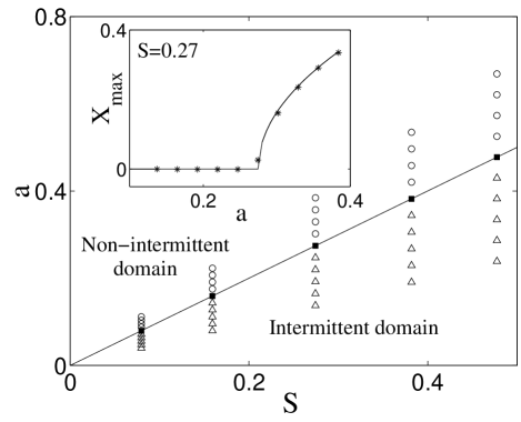
Figure 3: Boundary of the intermittent domain above the threshold $a\geq 0$ in the $(S,a)$–plane. The open triangles $(\triangle)$ show the intermittent domain where the most probable value $X_{max}$ of the PDF of $X$ is null. The open circles $(\circ)$ show the non–intermittent domain where the most probable value $X_{max}$ is different from $0$. The full squares $(\blacksquare)$ indicate the values of the parameters for which $X_{max}$ differs from $0$ for the first time in our simulations performed using increasing values of $a$. The straight line $S=a$ is the expected boundary predicted by equation (5). The stars $(\ast)$ in the inset show the most probable value $X_{max}$, as obtained from the numerical simulations of equation (1); the full line in the inset is the theoretical expression $X_{max}=\sqrt{a(a-S)/(a+3(M-S))}~{}(a>S)$, which is derived from equation (5).

III.2 Deterministic and chaotic fluctuations as a noise

Up to now, the only fluctuating parameters we have considered are stochastic processes. However, it is tempting to test the prediction of equation (5) in the case of a deterministic but chaotic fluctuating parameter. The noise is calculated from the chaotic solution of the Lorenz system Lorenz . We thus solve

$$\dot{U}=-\sigma(U-Y)\,,\dot{Y}=rU-Y-UZ\,,\dot{Z}=UY-bZ\,,$$ (16)

and define $\zeta$ as

$$\zeta=\alpha\frac{(1-\mu)U_{n}+\mu\dot{U_{n}}}{c}\,,$$ (17)

where $c^{2}=<((1-\mu)U_{n}+\mu\dot{U_{n}})^{2}>$, $U_{n}=\frac{U-<U>}{\sqrt{<(U-<U>)^{2}>}}$ and $\dot{U_{n}}=\frac{\dot{U}-<\dot{U}>}{\sqrt{<(\dot{U}-<\dot{U}>)^{2}>}}$. Averages are now understood as long time averages. The role of $c$ is to insure that $\alpha$ is the amplitude of the noise, i.e., $\sqrt{<\zeta^{2}>}=\alpha$. The parameter $\mu$ is tuned between zero and one in order to change the value of the spectrum at zero-frequency. Indeed $\dot{U}$ being the derivative of $U$, its power spectrum at low frequencies is smaller than that of $U$. Increasing $\mu$ increases the magnitude of $\dot{U}$ and thus reduces the spectrum of the noise at low frequencies (and accordingly the value of $S$).

The equations (1, 16) are solved with matlab using the same methods as in section $3.1$. We choose $r=25$, $\sigma=10$ and $b=8/3$. The solution of equation (16) is then chaotic and we plot in figures 5 and 5 some time series of $X$ and $\zeta$. On-off intermittency disappears when $\mu$ increases and thus, accordingly, $S$ decreases. This effect is coherent with our former interpretation of the role of the zero frequency noise spectrum. Indeed we have $a/S=0.332$ for fig. 5a and $a/S=5.64$ for fig. 5d. We also compute numerically the PDF of $X$ and compare it with the expression given by (5). The results are plotted in fig. 6. There again, for small values of the noise amplitude, the agreement between the prediction and the numerical results is very good.

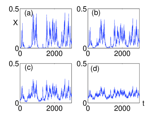
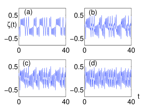
Figure 4: Solutions of equation (1) with $\zeta$ obtained from the Lorenz system (see figure 5). The departure from onset is $a=0.01$, the noise standard deviation is $\sqrt{<\zeta^{2}>}=0.2$. (a): $\mu=0$, (b): $\mu=0.5$, (c): $\mu=0.65$, (d): $\mu=0.8$.

Figure 5: Function $\zeta(t)$ obtained from the solution of the Lorenz system through equation (17). (a): $\mu=0$, (b): $\mu=0.5$, (c): $\mu=0.65$, (d): $\mu=0.8$. Note the difference in the horizontal scales $t$ with figure 5.

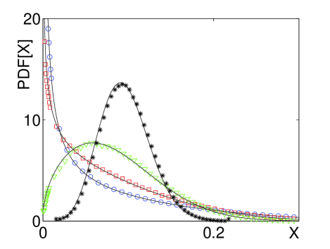
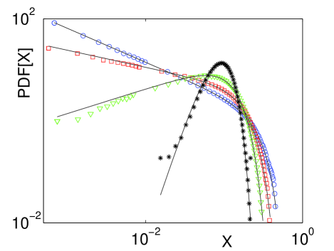
Figure 6: Top figure: Probability density function of the solutions of equation (1) when $\zeta(t)$ is obtained from the Lorenz system through equation (17). The parameter values are the same as those of figure 5: $a=0.01$, $\sqrt{<\zeta^{2}>}=0.2$. The continuous lines are the theoretical predictions given by equation (5). The symbols represent the numerical computation of the PDF: ($\circ$): $\mu=0$, ($\square$): $\mu=0.5$, ($\triangledown$): $\mu=0.65$, ($\ast$): $\mu=0.8$. Bottom figure: same results in loglog scale.

IV Statistics of the durations of the laminar phases

The intermittent regime can also be identified by the statistics of durations $\tau$ of the laminar phases close to zero (see e.g., fig.1a). We discuss in this section numerical results for the durations of the laminar phases, obtained by using the random process defined in equation (13).

In the close vicinity of the threshold, when $a\rightarrow 0^{+}$, a power law with an exponent $-3/2$ is expected for the PDF of $\tau$ Heagy . This is in agreement with fig.7 where we plot the PDF of $\tau$ for $S=0.159$ and for various values of $a$. The threshold under which $X$ is considered to be in the laminar state is chosen arbitrarily to be fifty times smaller than the noise intensity. However, we have verified that the PDF of $\tau$ does not depend strongly on this choice if the threshold remains small enough compared to the maximum of the bursts.

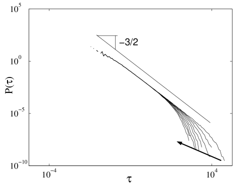
Figure 7: PDF of the duration $\tau$ of the laminar phases, for $S=0.159$ and $a$ varying from 0.008 to 0.0796 $(=S/2)$. The arrow indicates the curves for increasing values $a$.

We observe that the cut–off takes place at smaller values of $\tau$ when $a$ is increased. More precisely fig.8 shows that the PDF of $\tau$ can be fitted by

$$P(\tau)\propto\tau^{-3/2}.\exp(-\tau/\theta_{c})\,,$$ (18)

where the characteristic time of the cut–off $\theta_{c}$ is proportional to $S/a^{2}$. Indeed, the upper right inset shows that $\log\left(P(\tau)\right)+3/2\log(\tau)$ is linear with $\tau$ in agreement with (18). Moreover, the central curve shows that all the characteristic times $\theta_{c}$ collapse on a single line if they are plotted as a function of $a^{2}/S$.

This is in agreement with the exponential cut–off derived for white noise in Heagy ; Cenys . In the white noise case, the PDF of $\tau$ follows equation (18) with $\theta_{c}$ proportional to $D/a^{2}$ where D is the amplitude of the white noise. Our numerical studies show that in the limit of small $S$ this prediction remains valid for a non-white noise if $S$ is taken as the noise amplitude. Here again the noise power spectrum at zero frequency controls the value of $\theta_{c}$. As discussed in Part (VI.A), laminar phases occur when a random walk associated to the noise remains with the same sign for long durations. For small $S$ this property is controlled by the noise power spectrum at zero frequency.

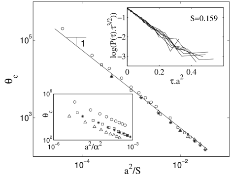
Figure 8: Characteristic time $\theta_{c}$ of the cut–off of the PDF of the laminar phase duration $\tau$, plotted as a function of $a^{2}/S$. The values of the parameter are $(\circ)$ : $S=0.0159,~{}\alpha^{2}=0.1$; $(\ast)$: $S=0.159,~{}\alpha^{2}=5.0$ ; $(\square)$ : $S=0.254,~{}\alpha^{2}=8$ and $(\triangle)$: $S=0.159,~{}\alpha^{2}=8$. The upper–right inset illustrates that the PDF of $\tau$ is well represented by (18). The lower–left inset shows that the collapse is not obtained if $\theta_{c}$ is plotted as a function of $a^{2}/\alpha^{2}$.

V Numerical simulations for a bifurcating system of second order in time

The Duffing oscillator and the effect of a multiplicative noise on its dynamics have been widely studied. Once the time is rescaled by the viscosity, the Duffing oscillator perturbed by a multiplicative noise can be written as

$$\ddot{X}+\dot{X}=(a+\xi)X-X^{3}\,.$$ (19)

Lücke and Schanck Lucke1 used an expansion valid for a small noise amplitude and close to the deterministic threshold. They showed that a small amount of multiplicative noise can stabilize the state $X=0$ for positive $a$, whereas in the deterministic case, $X=0$ is stable only for negative values of $a$. They calculated the threshold shift induced by the noise and found its expression as a function of the noise Power Density Spectrum. Their expansion leads to the usual behavior for the moments $\langle X^{2p}\rangle$ that are proportional to the departure from onset raised to the power $p$. We emphasize that their analysis is correct only for noise with a vanishing PSD at zero frequency Lucke2 . However, a recent study Kirone1 of the Duffing oscillator subject to Gaussian white noise or Ornstein-Uhlenbeck noise has predicted an intermittent behavior and a linear scaling of the moments $<X^{2p}>$ of the unstable variable with the departure from onset. In order to clarify this apparent contradiction between Refs. Lucke1 and Kirone1 and to investigate the effects of the low frequency part of the noise spectrum on the Duffing oscillator, we study numerically equation (19) with the colored noise defined by (13) for which the PSD is given by

$$S(\nu)=\frac{\alpha^{2}\eta(\Omega^{2}+\eta^{2})}{\pi[(\Omega^{2}+\eta^{2}-\nu^{2})^{2}+2\nu^{2}\eta^{2}]}\,.$$ (20)

Contrary to the case studied in Sections 2-4, the onset of instability is shifted by the noise. We thus have to take into account the new threshold $a_{c}$. For small noise amplitudes, this threshold is given by Lucke1

$$a_{c} = \int_{-\infty}^{+\infty}\frac{S(\nu)}{\nu^{2}+1/(2\pi)^{2}}d\nu\,,$$ (21)

$$= \frac{2\alpha^{2}(1+4\pi\eta)}{1+4\pi\eta+4\pi^{2}(\Omega^{2}+\eta^{2})}\,.$$ (22)

This theoretical result agrees with the numerical data (figure 9), taking into account the uncertainty in the numerical determination of the threshold.

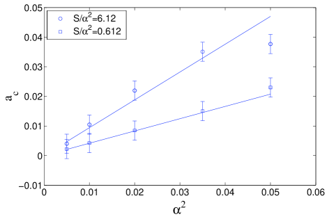
Figure 9: Instability threshold of equation (19) versus the noise intensity $\alpha^{2}$. The multiplicative noise is given by (14), with ($\circ$): $\eta=0.05$, $\Omega=0.01$ and ($\Box$) : $\eta=0.5$, $\Omega=0.1$. Full lines represent the theoretical result (22).

Figure 10 shows the temporal trace of $X(t)$ above onset. It emphasizes the fact that $S$ is still the pertinent parameter controlling the intermittent regime for small noise, i.e., for $\alpha^{2}<<1$. The same behavior is observed for the temporal trace of the other dynamical variable $\dot{X}(t)$.

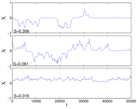
Figure 10: Temporal traces of the dynamical variable $X(t)$, solution of equation (19). In all cases $a-a_{c}=0.0754$, $\alpha^{2}=0.05$ and the autocorrelation function of the noise is given by (14), but $S$ is decreased from top to bottom.

Besides, figure 11 shows that the statistical behavior of the variable $E=X^{2}+\dot{X}^{2}$ is similar to that of the variable $X^{2}$ in the first order system studied in Sections 2-4. Indeed, the PDFs of $E$ divided by $E^{\gamma}$ with $\gamma=\frac{a-a_{c}}{2S}-1$ collapse on a single exponential for various values of $a$. Notice that the departure from the onset in the presence of noise must be taken into account. Therefore, when the amplitude of the noise is small, the PDF of the energy is controlled by the ratio between the departure from onset (in the presence of noise) and the value of the noise spectrum at zero frequency. When the amplitude of the noise is large, the PDF of the energy does not take the form suggested in fig. 11. However, even if the noise amplitude is large, on-off intermittency disappears when the value of $S$ is lowered.

To conclude this part, we point out that the failure of the perturbative expansion Lucke2 and the linear scaling of the moments as a function of the departure from onset Kirone1 are both a consequence of on-off intermittency that occurs when the noise is sufficiently large at low frequencies.

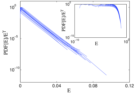
Figure 11: Probability Density Function of $E=X^{2}+\dot{X}^{2}$ divided by $E^{\gamma}$ with $\gamma=\frac{a-a_{c}}{2S}-1$ and for $\frac{a-a_{c}}{2S}$ going from 0.6 to 5.0. The inset in log–log plot underlines the plateau where the power law dominates the PDF.

VI Physical interpretations and summary

VI.1 Role of the low frequencies of the noise

In the different systems we have studied, on-off intermittency is controlled by the zero frequency component of the noise. Our interpretation of the phenomenon is the following. On-off intermittency occurs because of a competition between the noise and a systematic drift due to the departure from onset. More precisely, as pointed out in Yamada for the case of equation (1), when $X$ is close to the unstable manifold $X=0$, the evolution of $Y=\log{X}$ is given by $\dot{Y}=a+\zeta(t)$. For positive $a$, $\dot{Y}$ has a positive average but events in which $Y$ has a decreasing behavior are possible provided that $I=\int_{0}^{T}\zeta(t)dt/T$ remains smaller than $-a$ over a long duration. In the long time limit, the main contribution to the integral $I$ is due to the zero frequency component of the noise. If this component is reduced then occurrences of the inequality $I\leq-a$ become less and less probable and intermittency tends to be suppressed.

VI.2 Linearity of the moments

We now want to explain why, close to the onset of instability, all the moments vary linearly with $a$, the departure from onset. One can say that this is a direct consequence of the form of the PDFs that are power laws with exponents close to $-1$, the difference from $-1$ being proportional to $a$ (see equations (2), (5), (9)). However, we look here for an explanation based on the dynamical properties of the trajectories $X(t)$.

In the small $a$ limit, the variable $X$ spends long durations in the off-phase and, from time to time, it takes non-zero values. A typical trajectory is sketched in fig. 12. Let $T_{i}$ be the duration of the $i$-th on-phase and $T_{e}=T_{1}+T_{2}+..$ be the total time spent in the on-phases during the measurement time $T$.

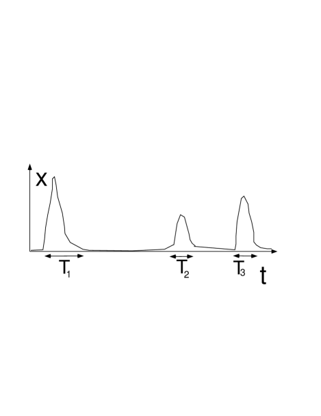
Figure 12: Sketch of the intermittent regime with $T_{i}$ the duration of the $i^{th}$ burst.

During the on-phases the evolution of $X$ can be described approximately by a random walk with a drift in terms of the variable $Y=\log{X}$; besides, the effect of nonlinearities can be modeled by a wall that prevents $Y$ from reaching too high values. Let us call $C_{n}$ the averaged value taken by $X^{n}$ during an on-phase. Using the fact that the off-phases have a negligible contribution to $\langle X^{n}\rangle$, we can write approximatively for a large measurement time $T$

$$\langle X^{n}\rangle=\frac{1}{T}\int_{0}^{T}X^{n}(t^{\prime})dt^{\prime}\simeq\frac{T_{e}}{T}C_{n}\,.$$ (23)

For large $T$, $T_{e}/T$ is the product of the averaged duration of an on-phase with the averaged frequency of occurrence of an on-phase. Using the aforementioned analogy with a biased random walk limited by a wall, we conclude that the averaged duration of an on-phase is finite when the drift $a$ tends to zero. Moreover, the averaged frequency of occurrence of an on-phase is proportional to $a$ and therefore $T_{e}/T$ is also proportional to $a$. This scaling law is tested numerically for equation (1) with Gaussian white noise. We plot in fig. 13 the quantity $T_{e}/T$ as a function of $a$ : The relation is linear when $a/D$ is small.

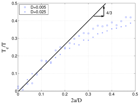
Figure 13: Total duration of the on–phase, $T_{e}$, normalized by the total duration of the measurement, $T$, as a function of the departure from the threshold, $a$, given for two values of the white noise intensity $\langle\xi(t)\xi(t^{\prime})\rangle=D\delta(t-t^{\prime})$.

Finally, $C_{n}$ the averaged value of the $n$-th moment of $X$ during the on-phase can be calculated in the case of a Gaussian white noise using eq. (5); $C_{n}$ tends to a non-zero constant when $a$ tends to zero. This fact can be understood using the analogy with the biased random walk limited by a wall: the typical trajectories restricted between the onset of the on-phase and the wall do not depend on $a$ for vanishing $a$.

To summarize, when $a$ is very small, the system enters on-phases with a frequency linear with $a$. However, the duration of these on-phases and the values reached by the system during these phases do not depend on $a$. Therefore, using eq. (23) and the above discussion, we conclude that

$$\langle X^{n}\rangle\propto a\,,$$ (24)

i.e., all the moments are linear with the departure from onset.

VI.3 Summary

We have studied different bifurcating systems subject to multiplicative noise. For a system of first order in time and for a small value of the product of the noise amplitude with its correlation time, an expansion showed that on-off intermittency occurs if the noise spectrum at zero frequency is greater than twice the departure from onset. This prediction is in agreement with numerical simulations that use colored random processes or chaotic fluctuations as noises. In the same limit we have shown that the statistics of the durations of the laminar phases are also controlled by the departure from onset and the noise spectrum at zero frequency. Even at finite amplitude of the noise, we have verified numerically that intermittency disappears when the low frequencies of the noise are filtered out. This result is also derived analytically for a Gaussian white noise and for another particular kind of noise, the dichotomous Markovian process. For a system of second order in time, we have numerically studied the behavior of the unstable variable and showed that for small noise amplitudes, the PDF of the energy scales as a power law with exponent controlled by the noise spectrum at zero frequency and the departure from the onset. Here again, by lowering the noise spectrum at zero frequency, the on-off intermittency is reduced and can be suppressed. Finally, we have given some physical explanations for the effect of the noise spectrum at zero frequency on on-off intermittency and for the behavior of all the moments of an on-off intermittent variable that are linear with the departure from onset.

This work has benefited from fruitful discussions with C. Van den Broeck, P. Marcq, N. Leprovost and S. Fauve.

Appendix : derivation of the cumulant expansion for a dynamical system of first order in time

If we consider one realization of the noise $\zeta(t)$ as a single time dependent forcing, then for a given initial condition $X(t=0)$, equation (1) describes a single trajectory. In other words, for a given realization of the noise, the number of trajectories in phase–space is conserved. A continuity equation for the density of trajectories in the phase–space $\rho_{\zeta}(X,t)$ can therefore be written VanKampen1 as follows :

$$\partial_{t}\rho_{\zeta}(X,t) = -\partial_{X}\left[\dot{X}\rho_{\zeta}(X,t)\right]$$ (25)

$$= -\partial_{X}\left[(aX-X^{3})\rho_{\zeta}(X,t)\right]$$

$$-\alpha\partial_{X}\left[F_{\zeta}(X,t)\rho_{\zeta}(X,t)\right]\,,$$

where $\alpha$ is the standard deviation of the noise and

$$F_{\zeta}(X,t)=\zeta(t)X(t)/\alpha.$$

The PDF of $X(t)$ is just the average of $\rho_{\zeta}(X,t)$ over all the realizations of the noise. Therefore, by averaging eq. (25), an evolution equation for $P(X,t)$ can be derived. Some approximations are however necessary to obtain an equation which is closed with respect to $P(X,t)$. In VanKampen1 (pp 210), Van Kampen expands equation ($25$) in powers of the parameter $\epsilon=\alpha^{2}\tau_{c}$ where $\tau_{c}$ is the correlation time of the noise. Assuming that $\epsilon<<1$ and knowing that $\langle F_{\zeta}(X,t)\cdot F_{\zeta}(X^{\prime},t^{\prime})\rangle\sim 0$ for $|t-t^{\prime}|>\tau_{c}$, the following equation for $P(X,t)$ is derived :

$$\partial_{t}P(X,t)=-\partial_{X}\left[-(aX-X^{3})P(X,t)\right]$$ (26)

$$-\alpha^{2}\partial_{X}\left\{\left[\int_{0}^{\infty}\langle\frac{\partial F_{\zeta}(X,t)}{\partial X}F_{\zeta}(X^{-\tau},t-\tau)\rangle\left|\frac{dX}{dX^{-\tau}}\right|\right]P(X,t)\right\}$$

$$-\alpha^{2}\partial^{2}_{XX}\left\{\left[\int_{0}^{\infty}\langle F_{\zeta}(X,t)F_{\zeta}(X^{-\tau},t-\tau)\rangle\left|\frac{dX}{dX^{-\tau}}\right|\right]P(X,t)\right\}\,,$$

where $X^{-\tau}=X_{o}(t-\tau)$ is the deterministic backward position, i.e., $X^{-\tau}$ represents the value of the variable $X$ at time $(t-\tau)$ such that $X$ would evolve upto $X_{o}(t)$ during the duration $\tau$ if there were no noise. The quantity $\left|\frac{dX}{dX^{-\tau}}\right|$ is the Jacobian of $X$ with respect to $X^{-\tau}$. Equation ($26$) is a second order expansion in power of the small parameter $\epsilon=\alpha^{2}\tau_{c}$ and is therefore valid as long as $\epsilon<<1$.

For equation (1), all the quantities such as $X^{-\tau}$ and the Jacobian can be explicitely calculated. By solving (1) with $\zeta(t)=0$, we find that

$$X = \pm\left\{\left[(a(X^{-\tau})^{-2}-1)\exp(-2a\tau)+1\right]/a\right\}^{-1/2}\,,$$

$$X^{-\tau} = \pm\left\{\left[(aX^{-2}-1)\exp(2a\tau)+1\right]/a\right\}^{-1/2}\,,$$

$$\left|\frac{dX}{dX^{-\tau}}\right| = (X/X^{-\tau})^{3}\,.$$

Finally, equation (3) is obtained by substituting the expressions for $\left|\frac{dX}{dX^{-\tau}}\right|$ and $X^{-\tau}$ in equation ($26$) and writing $F_{\zeta}(X,t)=\zeta(t)X(t)/\alpha$.

References

- (1) N.G. van Kampen, Physics Reports 24 171 (1976).
- (2) M. Neufeld, R. Friedrich, Phys. Rev. E, 51, 2033 (1995).
- (3) D. Sweet, E.Ott, J.M. Finn, T.M. Antonsen Jr, D.P. Lathrop, Phys. Rev. E, 63, 066211 (2001), D. Sweet, E.Ott, T.M. Antonsen Jr, D.P. Lathrop, J.M. Finn, Phys. Plasma, 8, 1944 (2001). S. Fauve and F. Pétrélis, “The dynamo effect”, pp. 1-66, “Peyresq Lectures on Nonlinear Phenomena, Vol. II”, Ed. J-A Sepulchre, World Scientific (Singapour, 2003).
- (4) R.L Stratonovich, Topics in the Theory of Random Noise (Gordon and Breach, New–York, 1963).
- (5) T. Kawakubo, S. Kabashima, Y. Tsuchiya, Prog. Theor. Phys. supp., 64, (1978).
- (6) A. Schenzle, H. Brand, Phys. Rev. A, 20, 1628 (1979), R. Graham, A. Schenzle, Phys. Rev. A, 26, 1676 (1982).
- (7) W. Horsthemke, R. Lefever, Noise-Induced Transitions (Springer-Verlag, 1984).
- (8) T. Yamada, H. Fujisaka, Prog. Theor. Phys., 76, 582 (1986), H. Fujisaka, H. Ishii, M. Inoue, T. Yamada, Prog. Theor. Phys., 76, 1198 (1986), N. Platt, E. A. Spiegel and C. Tresser, Phys. Rev. Lett. 70 (3) 279-282 (1993).
- (9) P. W. Hammer, N. Platt, S. M. Hammel, J. F. Heagy and B. D. Lee, Phys. Rev. Lett. 73, 1095 (1994), T. John, R. Stannarius and U. Behn, Phys. Rev. Lett. 83, 749 (1999), D. L. Feng, C. X. Yu, J. L. Xie and W. X. Ding, Phys. Rev. E 58, 3678 (1998), F. Rödelspreger, A. Cenys and H. Benner, Phys. Rev. Lett. 75, 2594 (1995).
- (10) S. Aumaître, F. Pétrélis and K. Mallick, Phys. Rev. Lett. 95, 064101 (2005).
- (11) M. Lücke, F. Schanck, Phys. Rev. Lett., 54, 1465 (1985).
- (12) K. Mallick, P. Marcq, Euro. Phys. J. B, 38, 99 (2004).
- (13) F. Pétrélis and S. Aumaître, Eur. Phys. J. B 34, 281-284 (2003).
- (14) N.G. van Kampen, Stochastic Process in Physics Chemistry , North-Holland, Amsterdam, 1992.
- (15) A. Teubel, U. Behn and A. Kühnel, Zeitschrift für Physik B-Condensed Matter 71, 393-402 (1988). I. Bena, C. Van Den Broeck, R. Kawai and K. Lindenberg, Phys. Rev. E 66, 045603(R) (2002). We are indebted to C. Van den Broeck for suggesting us the calculation presented in part 2.3.
- (16) B.L. Sawford, Phys. Fluids A, 3, 1577 (1991).
- (17) This expression corrects a misprint for defined in nous .
- (18) M. Lücke, Noise in nonlinear dynamical systems, Vol 2, Ed. F. Moss & P.V.E. McClintock, Cambridge University Press, 1989.
- (19) J.F. Heagy, N. Platt, S.M. Hammel, Phys. Rev. E, 49, 1140 (1994).
- (20) A. Čenys, A.N. Anagnopoulos, G.L. Bleris, Phys Lett. A, 224,346 (1997).
- (21) E. Lorenz, Journal of the Atmospheric Sciences, 20, 244 (1963).