Electric-field-induced displacement of a charged spherical colloid embedded in an elastic Brinkman medium

Abstract

When an electric field is applied to an electrolyte-saturated polymer gel embedded with charged colloidal particles, the force that must be exerted by the hydrogel on each particle reflects a delicate balance of electrical, hydrodynamic and elastic stresses. This paper examines the displacement of a single charged spherical inclusion embedded in an uncharged hydrogel. We present numerically exact solutions of coupled electrokinetic transport and elastic-deformation equations, where the gel is treated as an incompressible, elastic Brinkman medium. This model problem demonstrates how the displacement depends on the particle size and charge, the electrolyte ionic strength, and Young’s modulus of the polymer skeleton. The numerics are verified, in part, with an analytical (boundary-layer) theory valid when the Debye length is much smaller than the particle radius. Further, we identify a close connection between the displacement when a colloid is immobilized in a gel and its velocity when dispersed in a Newtonian electrolyte. Finally, we describe an experiment where nanometer-scale displacements might be accurately measured using back-focal-plane interferometry. The purpose of such an experiment is to probe physicochemical and rheological characteristics of hydrogel composites, possibly during gelation.

1 Introduction

Hydrogels are soft, water-saturated networks of polymer with molecular-scale porosity. They find widespread use in molecular-separation technologies (gel electrophoresis), drug delivery, scaffolds for tissue engineering, cell culture, wound care (e.g., Lowman et al., 2004; Yui et al., 2004), and microfluidic pumping and control (e.g., Bassetti et al., 2005).

This paper concerns a novel class of hydrogel composites where charged colloidal inclusions are immobilized in an uncharged hydrogel matrix. Matos et al. (2006) recently demonstrated that polyacrylamide hydrogels doped with silica nanoparticles significantly enhance the electric-field-induced transport of both charged and uncharged molecules through the composite. The underlying electroosmotic flow mechanism is consistent with theoretical expectations for weak perturbations to equilibrium (Hill, 2006c).

Each charged inclusion experiences electrical, hydrodynamic and mechanical contact forces, while the mobile counter charge produces an electro-osmotic flow that permeates the surrounding polymer. Hill (2006c) recently developed an electrokinetic transport model that quantifies how the charge and size of the inclusions, the ionic strength of the electrolyte, and gel permeability influence the electro-osmotic pumping capacity of an uncharged polymer network with randomly dispersed, impenetrable inclusions. To a first approximation, the elastic distortion of the network does not influence the flow or ion fluxes, so little is known of the particle displacements and flow-induced distortion of the polymer.

The particle displacement could be used as a diagnostic to probe the physicochemical characteristics of the particle-polymer interface, much like the electric-field-induced particle velocity (electrophoretic mobility) is used to infer the so-called $\zeta$-potential of colloidal particles dispersed in Newtonian electrolytes. Also, knowledge of the micro-scale strain field in the hydrogel is essential for establishing the electric field strength required to initiate micro-scale fracture. Finally, the relationship between particle displacement and the elastic and viscous characteristics of the surrounding matrix is central to the rapidly advancing field of micro-rheology, which seeks to quantify the dynamics and structure of complex fluids (Solomon & Lu, 2001; Willerbacher & Oelschlaeger, 2007). In this work, our principal objective is to quantify how the particle, electrolyte and hydrogel characteristics influence the electric-field-induced particle displacement.

As a first step, we solve a model problem where classical electrokinetic transport processes are coupled to the deformation of an incompressible isotropic, homogeneous porous medium. The analysis is restricted to situations where the applied electric field is uniform and weak, so the particle displacement is small and perturbations to equilibrium may be linearized accordingly. In this manner, our approximations are similar to those widely adopted in the classical theories of micro-electrophoresis (Russel et al., 1989) and other phoretic motion (Anderson, 1989). Nevertheless, our calculations are not restricted by the magnitude of the particle $\zeta$-potential or the thickness of the equilibrium diffuse layer of counterions (Debye length).

One promising approach to measure small particle displacements induced by an electric field involves collecting light scattered from a micron-sized inclusion at the focus of an optical trap. Back-focal-plane interferometry (e.g., Gittes et al., 1997; Schnurr et al., 1997; Allersma et al., 1998) provides nanometer-resolution position detection with $1$–$10^{4}$ Hz temporal resolution. The technique has been successfully applied to measure $0.1$–$100$ nm displacements of colloidal inclusions in complex fluids (e.g., polymer solutions and colloidal dispersions) and hydrogels, as well as the electric-field-induced velocity (electrophoretic mobility) of colloidal spheres dispersed in Newtonian electrolytes (e.g., Galneder et al., 2001). Reviews by MacIntosh (1999) and Furst (2005) present authoritative perspectives of the motivations, development and achievements of micro-rheology, with emphasis on single-particle dynamics and the use of optical traps.

The elastic restoring force of stiff gels significantly attenuates Brownian fluctuations in the position of colloidal particulates trapped in the hydrogel skeleton. Accordingly, passive micro-rheological techniques are well suited, and indeed limited, to weak gels. Schnurr et al. (1997) showed that the mean-squared displacement of a particle with radius $a$ trapped in an incompressible elastic matrix with Young’s modulus ${\cal E}$ is $kT/(2\pi a{\cal E})$ ($kT$ is the thermal energy). With $a=500$ nm and ${\cal E}=10$ kPa, for example, the mean-squared displacement is $\approx 0.4$ nm. Therefore, to register larger displacements in stiffer matrices, active micro-rheology typically adopts magnetic or optical forces to promote oscillatory particle motion. For example, Yamaguchi et al. (2005) recently demonstrated the use of a lock-in amplifier to correlate the particle response in an harmonic optical trap to resolve extraordinarily small displacements over a wide frequency range. This proved successful for following the transformation (gelation) of viscous polymer solutions to moderately stiff visco-elastic hydrogels.

Galneder et al. (2001) demonstrated the use of electrical forces to facilitate single-particle micro-electrophoresis studies. Their experiments produced $\sim 1$ $\mu$m s^-1 particle velocities in Newtonian electrolytes at $\sim 10$–$10^{2}$ Hz. Evidently, $\sim 10$–$100$ nm particle displacements were sufficient to measure the electrophoretic mobility. In principle, however, smaller electric-field-induced displacements could be resolved by correlating the response (particle displacement) with the applied electric field.

Accordingly, we complement our principal theoretical results with a description of a novel experiment that correlates the forcing and response time series when an electric field is used to impart quasi-steady oscillatory motion of a charged sphere embedded in a hydrogel. Because the electric-field-induced displacement reflects the size and charge of the inclusions, and the ionic strength of the electrolyte, this experiment could probe physicochemical changes at the inclusion-hydrogel interface. These are not registered using conventional laser-tweezer micro-rheology (e.g., Valentine et al., 1996; Yamaguchi et al., 2005) because the optical force of the trap, hydrodynamic drag of the electrolyte, and the elastic restoring force of an (uncharged) gel are (to a reasonable first approximation) independent of the inclusion surface charge (Gittes et al., 1997; Levine & Lubensky, 2001b).

The theoretical interpretation of such experiments may be complicated by several practical considerations and a variety of interesting physical phenomena. For example, if large electric fields are required to produce measurable particle displacements, then non-linear electro-kinetic influences, such as electroosmosis of the second kind (e.g., Mishchuk & Takhistov, 1995) and induced-charge electroosmosis (e.g., Bazant & Squires, 2004) come into play. Aided by experiments, Mishchuk & Takhistov (1995) demonstrated that electroosmosis of the second kind is significant when the applied (uniform) electric field $E>25kT/(ae)$ ($e$ is the fundamental charge, so $kT/e\approx 25$ mV at room temperature). It follows that a linearized electrokinetic model, such as the one pursued in this paper, should be reasonable for particles with radius $a=500$ nm when $E\lesssim 13$ kV cm^-1. Depending on the electrolyte conductivity, Joule heating may become problematic, so lower field strengths are obviously desirable.

Experiments may also be complicated by electrochemical reactions at the electrodes. These influences can be minimized by adopting time-dependent (oscillatory) electric fields, as exploited in electroacoustic (e.g., O’Brien, 1988) and dielectric relaxation (e.g., DeLacey & White, 1981) diagnostic experiments for colloidal dispersions, and electrically guided colloidal assembly processes (e.g., Ristenpart et al., 2007). Extending the present quasi-steady theory to handle oscillatory electric fields at frequencies where dynamics are important is a significant challenge. For example, several disparate length scales present an extremely ‘stiff’ computational problem, and dissipative wave-like dynamics are expected from the coupling of viscous (electrolyte) and elastic (polymer) phases.

Other interesting complications, which are not unique to the proposed electrically forced micro-rheology experiments, arise from polymer inhomogeneity (e.g., Maggs, 1998; Huh & Furst, 2006) and the degree of sticking and slipping at the particle-hydrogel interface. In principle, these influences can be integrated into the present computational methodology with appropriate modifications of the boundary conditions at the particle-polymer interface, and by allowing the elastic modulus and hydrodynamic permeability of the polymer skeleton to vary with radial position (e.g., Levine & Lubensky, 2001b; Chen et al., 2003). At present, however, these complications are of secondary importance to the task of understanding electrokinetic influences with homogeneous polymer.

Finally, our analysis concerns uncharged polymer networks. While many hydrogel skeletons, especially those of biological origin, bear fixed charge, poly(acrylamide) and poly(ethylene oxide) hydrogels, for example, as well as physical gels from block copolymers, are, at least in principle, uncharged (Lowman et al., 2004; Yui et al., 2004). Note that electric-field-induced actuation of hydrogels is limited exclusively to poly-electrolyte (intrinsically charged) hydrogels, which often respond to relatively weak electric fields ($E\sim 10$ V cm^-1) (Shiga, 1997). Although our primary concern is with micro-rheology, our theory may contribute to understanding how micro-scale transport processes influence macro-scale deflection (electrical actuation) of uncharged hydrogel skeletons that are endowed with charge from particulate inclusions.

Before presenting the full model and examining the results, it is instructive to first consider the expected displacement $Z$ of an inclusion if the bare electrical force $\sigma 4\pi a^{2}E$ is balanced by an elastic restoring force $2\pi a{\cal E}Z$. Here, $\sigma$ is the surface charge density, $4\pi a^{2}$ is the surface area, $E$ is the electric-field strength, and ${\cal E}$ is Young’s modulus of the gel. Accordingly, the particle displacement is

$$Z=2\sigma a{\cal E}^{-1}E.$$ (1)

Equation (1) over-estimates the displacement by a factor of $(2/3)\kappa a$ when $\kappa a\rightarrow\infty$ and $|\zeta|<kT/e$. Note that $\kappa a$ is the particle radius $a$ scaled with the Debye length $\kappa^{-1}$, $\zeta$ is the $\zeta$-potential, $kT$ is the thermal energy, and $e$ is the fundamental charge. When $\kappa a\rightarrow 0$ and $|\zeta|<kT/e$, however, Eqn. (1) becomes

$$Z=2\zeta\epsilon_{s}\epsilon_{o}{\cal E}^{-1}E\ \ (\kappa a\rightarrow 0,|\zeta|<kT/e).$$ (2)

Equation (2) and the correct form of Eqn. (1) for $\kappa a\rightarrow\infty$ (see section 5) are, respectively, reminiscent of the well-known Hückel and Smoluchowski limits for the electrophoretic mobility (Russel et al., 1989). Indeed, despite obvious differences, the inclusion displacement and electrophoretic velocity have a remarkably similar and, in general, complicated dependence on the scaled particle size $\kappa a$ and scaled $\zeta$-potential $\zeta e/(kT)$.

2 Models for electrokinetic transport and elastic deformation

As depicted in figure 1, we consider a single spherical colloid with radius $a$ and surface charge density $\sigma$ embedded in an unbounded, electrically neutral hydrogel. The gel is modeled as a homogeneous Brinkman medium that is saturated with an aqueous electrolyte (e.g., NaCl). Together, the electrolyte concentration, surface charge density and particle radius manifest as an electrostatic potential $\zeta$ at the colloid surface ($r=a$). Note that the counter-charge is concentrated in a diffuse layer with thickness (Debye length) $\kappa^{-1}$.

Figure 1: Schematic representation of a (negatively) charged, spherical colloid embedded in an unbounded electrolyte-saturated, elastic polymer gel (elastic Brinkman medium). An electric field $E$ is applied that drives electro-osmotic flow $u$, which, in turn, exerts a body force on the gel that induces a displacement field $v$. The net result of the electrical, hydrodynamic and elastic stress is a displacement $Z$ of the particle (to the left). The dashed lines denote the equilibrium (right) and polarized (left) diffuse double layers. In the far-field ($r\rightarrow\infty$), the velocity and displacement fields decay as $r^{-3}$. In this work, the displacement field is treated as the sum of two fields that each decay as $r^{-1}$; one is induced by a particle displacement $\mbox{\boldmath$Z$\unboldmath}\neq\mbox{\boldmath$0$\unboldmath}$ with $\mbox{\boldmath$E$\unboldmath}=\mbox{\boldmath$0$\unboldmath}$, and the other is the flow-induced distortion with $\mbox{\boldmath$E$\unboldmath}\neq\mbox{\boldmath$0$\unboldmath}$ and $\mbox{\boldmath$Z$\unboldmath}=\mbox{\boldmath$0$\unboldmath}$.

2.1 Electrokinetic transport

The electrokinetic model used in this work to calculate the equilibrium and perturbed electrolyte ion concentrations, pressure, and fluid velocity is a straightforward extension of the standard electrokinetic model (Booth, 1950) widely used to describe micro-electrophoresis and other electrokinetic phenomena. Details have been presented elsewhere (Hill, 2006c, b). The full set of (steady) transport equations is

$$\epsilon_{o}\epsilon_{s}\nabla^{2}\psi=-\sum_{j=1}^{N}n_{j}z_{j}e$$ (3)

$$\mbox{\boldmath$j$\unboldmath}_{j}=n_{j}\mbox{\boldmath$u$\unboldmath}-z_{j}en_{j}\frac{D_{j}}{kT}\mbox{\boldmath$\nabla$\unboldmath}\psi-D_{j}\mbox{\boldmath$\nabla$\unboldmath}{n_{j}}$$ (4)

$$\eta\nabla^{2}\mbox{\boldmath$u$\unboldmath}-\mbox{\boldmath$\nabla$\unboldmath}p=(\eta/{\ell}^{2})\mbox{\boldmath$u$\unboldmath}+\sum_{j=1}^{N}n_{j}z_{j}e\mbox{\boldmath$\nabla$\unboldmath}\psi,$$ (5)

with (steady) ion and electrolyte conservation equations

$$\mbox{\boldmath$\nabla$\unboldmath}\cdot{\mbox{\boldmath$j$\unboldmath}_{j}}=0\mbox{ and }\mbox{\boldmath$\nabla$\unboldmath}\cdot{\mbox{\boldmath$u$\unboldmath}}=0.$$

The electrostatic potential, $N$ ion concentrations and fluxes, electrolyte velocity, and pressure are denoted $\psi$, $n_{j}$ and $\mbox{\boldmath$j$\unboldmath}_{j}$, $u$, and $p$, respectively. Other variables are the solvent dielectric constant $\epsilon_{s}$, permitivity of a vacuum $\epsilon_{o}$, fundamental charge $e$, ion valances $z_{j}$ and diffusion coefficients $D_{j}$, thermal energy $kT$, solvent viscosity $\eta$, and Darcy permeability ${\ell}^{2}$ (square of the Brinkman (1947) screening length). Note that the double-layer thickness (Debye length) is

$$\kappa^{-1}=\sqrt{kT\epsilon_{s}\epsilon_{o}/(2Ie^{2})},$$

where $I=(1/2)\sum_{j=1}^{N}z^{2}_{j}n^{\infty}_{j}$ is the bulk ionic strength, with $n_{j}^{\infty}$ the bulk ion concentrations. Since this work deals exclusively with steady (or quasi-steady) flows, the fluid velocity in Eqn. (5) is relative to a stationary polymer skeleton.

The equations are solved by perturbing (to linear order) from an equilibrium base state where $\mbox{\boldmath$u$\unboldmath}=\mbox{\boldmath$0$\unboldmath}$ and the equilibrium electrostatic potential, ion concentrations and pressure are denoted $\psi^{0}$, $n_{j}^{0}$, and $p^{0}$, respectively (O’Brien & White, 1978; Hill et al., 2003). With the application of a uniform electric field $E$,

$$\psi=\psi^{0}+\psi^{\prime},\ n_{j}=n_{j}^{0}+n_{j}^{\prime},\ \mbox{\boldmath$u$\unboldmath}=\mbox{\boldmath$u$\unboldmath}^{\prime},$$

where

$$\psi^{\prime}=-\mbox{\boldmath$E$\unboldmath}\cdot\mbox{\boldmath$r$\unboldmath}+\hat{\psi}(r)\mbox{\boldmath$E$\unboldmath}\cdot\mbox{\boldmath$e$\unboldmath}_{r},\ n_{j}^{\prime}=\hat{n}_{j}(r)\mbox{\boldmath$E$\unboldmath}\cdot\mbox{\boldmath$e$\unboldmath}_{r},$$

and

$$u = \mbox{\boldmath$\nabla$\unboldmath}\times\mbox{\boldmath$\nabla$\unboldmath}\times f(r)\mbox{\boldmath$E$\unboldmath}$$ (6)

$$= -2f_{r}r^{-1}(\mbox{\boldmath$E$\unboldmath}\cdot\mbox{\boldmath$e$\unboldmath}_{r})\mbox{\boldmath$e$\unboldmath}_{r}-(f_{rr}+f_{r}r^{-1})(\mbox{\boldmath$E$\unboldmath}\cdot\mbox{\boldmath$e$\unboldmath}_{\theta})\mbox{\boldmath$e$\unboldmath}_{\theta}.$$

Here, $f_{r}=\mbox{d}f/\mbox{d}r$, $f_{rr}=\mbox{d}^{2}f/\mbox{d}r^{2}$, $r$ is position in a spherical polar coordinate system $(r,\theta,\phi)$ with unit basis vectors ($\mbox{\boldmath$e$\unboldmath}_{r},\mbox{\boldmath$e$\unboldmath}_{\theta},\mbox{\boldmath$e$\unboldmath}_{\phi})$, and $\mbox{\boldmath$e$\unboldmath}_{z}$ is the orientation of the polar axis (so $\mbox{\boldmath$e$\unboldmath}_{r}\cdot\mbox{\boldmath$e$\unboldmath}_{z}=\cos{\theta}$).

At the particle-electrolyte interface ($r=a$),

$$\mbox{\boldmath$u$\unboldmath}=\mbox{\boldmath$0$\unboldmath}\ (\mbox{no slip}),\ \mbox{\boldmath$j$\unboldmath}_{j}\cdot\mbox{\boldmath$e$\unboldmath}_{r}=0\ (\mbox{no flux}),$$

and

$$\epsilon_{s}\epsilon_{o}\mbox{\boldmath$\nabla$\unboldmath}_{>}{\psi}\cdot\mbox{\boldmath$e$\unboldmath}_{r}-\epsilon_{p}\epsilon_{o}\mbox{\boldmath$\nabla$\unboldmath}_{<}{\psi}\cdot\mbox{\boldmath$e$\unboldmath}_{r}=-\sigma\ (\mbox{constant surface charge}),$$

where $\epsilon_{p}$ is the particle dielectric constant, and $\sigma$ is the (constant) surface charge density; the subscripts attached to the gradient operators distinguish the particle ($<$) and solvent ($>$) sides of the interface.

In the far-field ($r\rightarrow\infty$),

$$\psi \rightarrow -\mbox{\boldmath$E$\unboldmath}\cdot\mbox{\boldmath$r$\unboldmath}+(\mbox{\boldmath$E$\unboldmath}\cdot\mbox{\boldmath$e$\unboldmath}_{r})D^{E}r^{-2}$$

$$n_{j} \rightarrow n_{j}^{\infty}+(\mbox{\boldmath$E$\unboldmath}\cdot\mbox{\boldmath$e$\unboldmath}_{r})C^{E}_{j}r^{-2}$$

$$u \rightarrow -2C^{E}r^{-3}(\mbox{\boldmath$E$\unboldmath}\cdot\mbox{\boldmath$e$\unboldmath}_{r})\mbox{\boldmath$e$\unboldmath}_{r}-C^{E}r^{-3}(\mbox{\boldmath$E$\unboldmath}\cdot\mbox{\boldmath$e$\unboldmath}_{\theta})\mbox{\boldmath$e$\unboldmath}_{\theta},$$ (7)

where the scalar coefficients $D^{E}$, $C_{j}^{E}$ and $C^{E}\eta/{\ell}^{2}$ are, respectively, the dipole strengths of the electrostatic potential, ion concentrations, and pressure perturbations, induced by the electric field. Note that the far-field flow is a Darcy flow, $\mbox{\boldmath$u$\unboldmath}=-({\ell}^{2}/\eta)\mbox{\boldmath$\nabla$\unboldmath}{p^{\prime}}$, decaying as $r^{-3}$ as $r\rightarrow\infty$.

The full equations and boundary conditions above are the basis of an efficient numerical solution that yields the so-called asymptotic coefficients $D^{E}$, $C_{j}^{E}$ and $C^{E}$, which have been used to calculate the bulk electrical conductivity and pore mobility of dilute polymer-gel composites (Hill, 2006c, a). This work draws upon $C^{E}$, and introduces a new asymptotic coefficient $Z^{E}$ to characterize the far-field decay of the electric-field-induced elastic displacement field.

2.2 Elastic deformation

Elastic deformation of the polymer gel is calculated by modeling the polymer skeleton as an elastic Brinkman medium, whose equation of static equilibrium is

$$\mbox{\boldmath$\nabla$\unboldmath}\cdot{\mbox{\boldmath$\sigma$\unboldmath}}+(\eta/{\ell}^{2})\mbox{\boldmath$u$\unboldmath}=\mbox{\boldmath$0$\unboldmath}.$$ (8)

Here, the elastic stress tensor is (Landau & Lifshitz, 1986)

$$\mbox{\boldmath$\sigma$\unboldmath}=\frac{{\cal E}}{(1+\nu)}[\mbox{\boldmath$e$\unboldmath}+\frac{\nu}{(1-2\nu)}(\mbox{\boldmath$\nabla$\unboldmath}\cdot{\mbox{\boldmath$v$\unboldmath}})\mbox{\boldmath$\delta$\unboldmath}],$$ (9)

where $v$ is the (small-amplitude) displacement, ${\cal E}$ is Young’s modulus, $\nu$ is Poisson’s ratio, $\mbox{\boldmath$e$\unboldmath}=(1/2)[\mbox{\boldmath$\nabla$\unboldmath}{\mbox{\boldmath$v$\unboldmath}}+(\mbox{\boldmath$\nabla$\unboldmath}{\mbox{\boldmath$v$\unboldmath}})^{T}]$, and $\delta$ is the identity tensor. Substituting Eqn. (9) into Eqn. (8) gives

$$\frac{{\cal E}}{2(1+\nu)}\nabla^{2}{\mbox{\boldmath$v$\unboldmath}}+\frac{{\cal E}}{2(1+\nu)(1-2\nu)}\mbox{\boldmath$\nabla$\unboldmath}{(\mbox{\boldmath$\nabla$\unboldmath}\cdot{\mbox{\boldmath$v$\unboldmath}})}=-(\eta/{\ell}^{2})\mbox{\boldmath$u$\unboldmath}.$$ (10)

Again, the fluid velocity is relative to a stationary polymer skeleton ($\partial\mbox{\boldmath$v$\unboldmath}/\partial t=\mbox{\boldmath$0$\unboldmath}$).

When the (leading order) displacement is divergence-free, which is the situation addressed throughout this paper, deformation can only influence the (isotropic) permeability tensor $(\eta/{\ell}^{2})\mbox{\boldmath$\delta$\unboldmath}$ by inducing anisotropy. Note that any deformation-induced change in permeability yields a non-zero product of the permeability perturbation and the fluid velocity, the later of which is itself a perturbation. Accordingly, these second-order terms are neglected in the present (linearized) theory.

There is also a possibility of anisotropy in permeability due to the underlying random microstructure of the medium (hydrogel matrix), which itself is not isotropic at very small length scales. However, we assume this medium to be statistically isotropic and homogeneous, so that, at the level of a Representative Volume Element (RVE) of the deterministic continuum, the anisotropy vanishes just as the fluctuations in constitutive response tend to zero; see Ostoja-Starzewski & Wang (1989) for a random elastic model. Such a scale-dependent homogenization (i.e., a passage from a random microstructure to the RVE) was recently studied in the context of Stokesian permeability (Du & Ostoja-Starzewski, 2006), albeit the departure from anisotropy was not addressed explicitly; see also Ostoja-Starzewski (2007) for related studies in many other material problems.

The Poisson ratios of several widely used, highly swollen, transparent hydrogels are reported greater than 0.45. In particular, poly(vinyl alcohol) hydrogels prepared with a mixed solvent of dimethyl sulfoxide and water have $\nu\approx 0.472$ (Urayama et al., 1993), and polyacrylamide hydrogels have $\nu\approx 0.457$ (Takigawa et al., 1996). However, it is important to note that these measurements are ascertained from macroscale experiments where the characteristic length and time scales cannot probe the equilibrium (long-time) state of strain. For example, the fractional change in volume after relaxing to equilibrium is $\delta V/L^{3}\sim(1-2\nu)l/L$, where the strain $l/L\ll 1$ is the ratio of the imposed displacement $l$ to the specimen size $L$. The flux of solvent flowing through the specimen during the so-called draining time $\tau$ is $u_{c}\sim\delta V/(L^{2}\tau)\sim(1-2\nu)l/\tau$. Further, the flux is driven by a pressure gradient $p_{c}/L\sim(\eta/{\ell}^{2})u_{c}$, where, to balance the elastic stresses, the characteristic pressure is $p_{c}\sim{\cal E}(l/L)$. Together, the foregoing yield

$$\tau\sim(1-2\nu)(\eta/{\cal E})(L/{\ell})^{2},$$ (11)

so with $\eta\sim 10^{-3}$ Pas, ${\cal E}\sim 10^{5}$ Pa, $L\sim 10^{-2}$ m (macro-scale experiment) and ${\ell}\sim 10^{-9}$ m, the relaxation time is $\tau\sim(1-2\nu)10^{6}$ s. Clearly, this is extraordinarily long if $\nu$ is not sufficiently close to $0.5$. Accordingly, when the experimental time scale (e.g., reciprocal frequency) is shorter than the draining time, the change in volume will be smaller than at equilibrium, and the apparent Poisson ratio will be greater than the drained value.

In contrast, the draining time associated with the displacement of a microsphere ($L=a\sim 10^{-6}$ m) embedded in a hydrogel with ${\cal E}\sim 10^{5}$ Pa and ${\ell}\sim 10^{-9}$ m is only $\tau\sim(1-2\nu)10^{-2}$ s. Clearly, such an experiment is much better suited to probing the compressibility of the polymer skeleton. However, solving the problem with a compressible polymer matrix demands a distinctly different computational methodology than the one adopted in this paper for incompressible gels. Moreover, compressibility is anticipated to yield quantitative—not qualitative—changes in the calculated particle displacement. This expectation is supported, in part, by the fact that, in the absence of an electric field, the quasi-steady particle displacement varies by at most 25 percent from the incompressible limit as Poisson’s ratio spans the range $0$–$0.5$ (Schnurr et al., 1997). Clearly, a definitive answer requires a solution of the electrokinetic equations with arbitrary Poisson’s ratio: an ambitious goal that is beyond the relatively modest scope of the present work.

Finally, the density and, hence, rigidity of the inclusions (e.g., polymer latex or silica) are typically much greater than those of the gel. Accordingly, the inclusions are treated as rigid spheres. Moreover, the displacement field is assumed to be continuous across the inclusion-hydrogel interface. Other interfacial conditions include the possibility of (tangential) slip (e.g. Mura et al., 1985) or an opening crack, for example. The opening of a crack significantly complicates the analysis, and a slipping boundary condition is difficult to justify here, since it requires a physical mechanism to exert an interfacial radial stress while maintaining zero (relative) radial displacement and zero tangential stress. Accordingly, neither possibility is pursued here.

3 Superposition to calculate the particle displacement

It is convenient to calculate the electric-field-induced particle displacement $Z$ by superposing two linearly independent displacement fields.

One is the displacement field induced by a small displacement $Z$ of the inclusion in the absence of an electric field ($\mbox{\boldmath$E$\unboldmath}=\mbox{\boldmath$0$\unboldmath}$). There is no Darcy drag, and the solution of Eqn. (10) can be calculated analytically (see appendix A). The resulting mechanical-contact force exerted by the polymer on the particle is

$$\mbox{\boldmath$f$\unboldmath}^{m,Z}=-\frac{2\pi a{\cal E}\mbox{\boldmath$Z$\unboldmath}(1-\nu)}{(5/6-\nu)(1+\nu)}.$$ (12)

The other arises from the Darcy drag force when an electric field $E$ is applied and the inclusion is fixed at the origin ($\mbox{\boldmath$Z$\unboldmath}=\mbox{\boldmath$0$\unboldmath}$). The Darcy drag force in Eqn. (10) is calculated from the electrokinetic transport equations with a rigid polymer gel. Then the displacement can be obtained by solving Eqn. (10). This is detailed in section 4, where it is also shown that the mechanical-contact force exerted by the polymer on the inclusion is

$$\mbox{\boldmath$f$\unboldmath}^{m,E}=(8/3)\pi Z^{E}{\cal E}\mbox{\boldmath$E$\unboldmath}-4\pi(\eta/{\ell}^{2})C^{E}\mbox{\boldmath$E$\unboldmath}\ \ (\nu=1/2).$$ (13)

In addition to the net mechanical-contact force

$$\mbox{\boldmath$f$\unboldmath}^{m}=\mbox{\boldmath$f$\unboldmath}^{m,Z}+\mbox{\boldmath$f$\unboldmath}^{m,E},$$ (14)

there are electrical and hydrodynamic (drag) forces acting on the particle, denoted $\mbox{\boldmath$f$\unboldmath}^{e,E}$ and $\mbox{\boldmath$f$\unboldmath}^{d,E}$, respectively. These are already known from earlier solutions of the electrokinetic transport equations with a rigid (unperturbed) polymer gel (Hill, 2006b, c). Their sum can be written in terms of the asymptotic coefficient $C^{E}$ that characterizes the far-field decay of the electric-field-induced flow:

$$\mbox{\boldmath$f$\unboldmath}^{e,E}+\mbox{\boldmath$f$\unboldmath}^{d,E}=4\pi(\eta/{\ell}^{2})C^{E}\mbox{\boldmath$E$\unboldmath}.$$ (15)

Finally, static equilibrium of the particle demands

$$\mbox{\boldmath$f$\unboldmath}^{e,E}+\mbox{\boldmath$f$\unboldmath}^{d,E}+\mbox{\boldmath$f$\unboldmath}^{m,Z}+\mbox{\boldmath$f$\unboldmath}^{m,E}=\mbox{\boldmath$0$\unboldmath}.$$ (16)

Therefore, collecting the explicit expressions for the various forces above [Eqns. (12), (13) (with $\nu=1/2$) and (15)] gives the particle displacement

$$\mbox{\boldmath$Z$\unboldmath}=(4/3)(Z^{E}/a)\mbox{\boldmath$E$\unboldmath}\ \ (\nu=1/2).$$ (17)

The task of calculating $Z^{E}$ is detailed in the next section. Note that the contributions involving $C^{E}$ vanish, indicating that the slowest ($r^{-1}$) far-field decay of the displacement field vanishes upon superposition. In other words, there is no net force acting on the polymer, so the Darcy drag force exerted by the electrolyte on the polymer is counterbalanced by the mechanical-contact force exerted by the inclusion on the polymer. In a composite with a finite inclusion number density, or finite volume fraction $\phi$, part of the net mechanical-contact force acting on the polymer must be provided by a mechanical support to balance an accompanying $O(\phi)$ average pressure gradient (Hill, 2006c).

4 The electric-field-induced mechanical-contact force for an incompressible, elastic Brinkman medium

This section addresses the displacement induced by Darcy drag when an electric field is applied and the inclusion is fixed at the origin. This problem is adopted to calculate the force $\mbox{\boldmath$f$\unboldmath}^{m,E}$ appearing in Eqn. (13). Note that the numerical solution is limited to incompressible ($\mbox{\boldmath$\nabla$\unboldmath}\cdot{\mbox{\boldmath$v$\unboldmath}}=0$) displacement fields, so $\nu=1/2$.

In appendix B, the displacement field is expanded as a power series in a small parameter $\epsilon=1-2\nu$, i.e.,

$$\mbox{\boldmath$v$\unboldmath}=\mbox{\boldmath$v$\unboldmath}_{0}+\epsilon\mbox{\boldmath$v$\unboldmath}_{1}+....$$ (18)

The leading contribution to the displacement $\mbox{\boldmath$v$\unboldmath}_{0}$ is divergence-free ($\mbox{\boldmath$\nabla$\unboldmath}\cdot{\mbox{\boldmath$v$\unboldmath}_{0}}=0$) and satisfies the $O(\epsilon)$ equation of static equilibrium,

$$\nabla^{2}\mbox{\boldmath$v$\unboldmath}_{0}+\mbox{\boldmath$\nabla$\unboldmath}{(\mbox{\boldmath$\nabla$\unboldmath}\cdot{\mbox{\boldmath$v$\unboldmath}_{1}})}=-(\eta/{\ell}^{2})\mbox{\boldmath$u$\unboldmath}\frac{3}{{\cal E}}\ \ (\nu=1/2).$$ (19)

Incompressibility (as required by the $O(1)$ problem) is guaranteed by writing

$$\mbox{\boldmath$v$\unboldmath}_{0}=\mbox{\boldmath$\nabla$\unboldmath}\times{}\mbox{\boldmath$\nabla$\unboldmath}\times{}g(r)\mbox{\boldmath$E$\unboldmath},$$ (20)

where $g(r)$ is a function of radial position $r$. It follows that

$$\mbox{\boldmath$v$\unboldmath}_{0}=-2g_{r}r^{-1}(\mbox{\boldmath$E$\unboldmath}\cdot\mbox{\boldmath$e$\unboldmath}_{r})\mbox{\boldmath$e$\unboldmath}_{r}-(g_{rr}+g_{r}r^{-1})(\mbox{\boldmath$E$\unboldmath}\cdot\mbox{\boldmath$e$\unboldmath}_{\theta})\mbox{\boldmath$e$\unboldmath}_{\theta},$$ (21)

where, for example, $g_{r}=\mbox{d}g/\mbox{d}r$.

Because the fluid is also incompressible, its velocity field may be written as

$$\mbox{\boldmath$u$\unboldmath}=\mbox{\boldmath$\nabla$\unboldmath}\times{}\mbox{\boldmath$\nabla$\unboldmath}\times{}f(r)\mbox{\boldmath$E$\unboldmath},$$ (22)

where $f(r)$ is available from earlier work examining the influence of an electric field (Hill, 2006c) and a bulk concentration gradient (Hill, 2006b) with a rigid polymer gel ($\mbox{\boldmath$v$\unboldmath}=\mbox{\boldmath$0$\unboldmath}$).

If the deformation is assumed not to affect electrokinetic transport processes, which is a reasonable approximation when the displacement is divergence-free (so the polymer segment density and, hence, the Darcy permeability are unperturbed), then the earlier calculations also provide an exact solution with (weak) elastic deformation.

Substituting Eqns. (20) and (22) into the curl of Eqn. (19) gives

$$\frac{\mbox{d}}{\mbox{d}r}\nabla^{2}\nabla^{2}g+\frac{3\eta}{{\cal E}{\ell}^{2}}\frac{\mbox{d}}{\mbox{d}r}\nabla^{2}f=0,$$ (23)

where

$$\nabla^{2}=\frac{1}{r^{2}}\frac{\mbox{d}}{\mbox{d}r}(r^{2}\frac{\mbox{d}}{\mbox{d}r}),$$ (24)

and $f(r)$ is known. In this manner, $\mbox{\boldmath$v$\unboldmath}_{0}$ is decoupled from $\mbox{\boldmath$v$\unboldmath}_{1}$.

The fourth-order ordinary differential equation for $g_{r}(r)$ is solved numerically as two second-order differential equations:

$$\frac{\mbox{d}^{2}h}{\mbox{d}r^{2}}+\frac{4}{r}\frac{\mbox{d}h}{\mbox{d}r}-\frac{4}{r^{2}}h = -\frac{3\eta}{{\cal E}{\ell}^{2}}(\frac{\mbox{d}^{2}f_{r}}{\mbox{d}r^{2}}+\frac{2}{r}\frac{\mbox{d}f_{r}}{\mbox{d}r}-\frac{2}{r^{2}}f_{r})$$ (25)

$$\frac{\mbox{d}^{2}g_{r}}{\mbox{d}r^{2}} = h.$$ (26)

When the displacement is continuous across the inclusion-hydrogel interface, and vanishes in the far-field, the boundary conditions are

$$\mbox{\boldmath$v$\unboldmath}_{0}=\mbox{\boldmath$0$\unboldmath}\mbox{ at }r=a,$$ (27)

and

$$\mbox{\boldmath$v$\unboldmath}_{0}\rightarrow-2Z^{E}r^{-1}(\mbox{\boldmath$E$\unboldmath}\cdot\mbox{\boldmath$e$\unboldmath}_{r})\mbox{\boldmath$e$\unboldmath}_{r}-Z^{E}r^{-1}(\mbox{\boldmath$E$\unboldmath}\cdot\mbox{\boldmath$e$\unboldmath}_{\theta})\mbox{\boldmath$e$\unboldmath}_{\theta}\mbox{ as }r\rightarrow\infty.$$ (28)

The asymptotic coefficient $Z^{E}$ characterizes the strength of the $r^{-1}$ decay of $v$ (reflecting a net force). It follows that

$$g_{r}=g_{rr}=0\mbox{ at }r=a,$$ (29)

and

$$g_{r}\rightarrow Z^{E}\mbox{ and }g_{rr}\rightarrow 0\mbox{ as }r\rightarrow\infty.$$ (30)

An analytical boundary-layer analysis that solves the problem when $\kappa a\gg 1$, ${\ell}\ll a$ and $|\zeta|<kT/e$ serves to verify the numerical solution and to highlight the parametric scaling of $Z$. The result is presented in section 5 [Eqn. (39)], where we also examine numerically exact solutions of the full model.

Turning to the force, the leading contribution to the isotropic stress requires knowledge of the $O(\epsilon)$ displacement field $\mbox{\boldmath$v$\unboldmath}_{1}$, which is not divergence-free (see appendix B). Clearly, the divergence of $\mbox{\boldmath$v$\unboldmath}_{1}$ is necessary to evaluate the leading contribution to the force. Fortunately, the isotropic stress can be obtained from the solution of the $O(\epsilon)$ problem above. This is achieved by integrating Eqn. (78) once $\mbox{\boldmath$v$\unboldmath}_{0}$ is known. The task is simplified even further, because only the far-field decay of the displacement and fluid velocity fields are needed to evaluate the force. We have verified our general procedure by applying it to two simpler problems: one is the classical problem of Stokes flow past a sphere, and the other is the elastic restoring force on a rigid sphere embedded in an incompressible elastic continuum. Recall, the exact solution of the latter problem, for any $\nu$ [see Eqn. (12)], is worked out in appendix A.

The mechanical-contact force exerted by the polymer on the inclusion is

$$\mbox{\boldmath$f$\unboldmath}^{m,E}=\int_{r=a}\mbox{\boldmath$\sigma$\unboldmath}\cdot\hat{\mbox{\boldmath$n$\unboldmath}}\mbox{d}A=\int_{r\rightarrow\infty}\mbox{\boldmath$\sigma$\unboldmath}\cdot\hat{\mbox{\boldmath$n$\unboldmath}}\mbox{d}A+\int_{r=a}^{\infty}(\eta/{\ell}^{2})\mbox{\boldmath$u$\unboldmath}\mbox{d}V.$$ (31)

Note that (see appendix B)

$$\mbox{\boldmath$\sigma$\unboldmath}=\frac{2{\cal E}}{3}[\mbox{\boldmath$e$\unboldmath}_{0}+\frac{1}{2}(\mbox{\boldmath$\nabla$\unboldmath}\cdot{\mbox{\boldmath$v$\unboldmath}_{1}})\mbox{\boldmath$\delta$\unboldmath}],$$ (32)

where $\mbox{\boldmath$e$\unboldmath}_{0}=(1/2)[\mbox{\boldmath$\nabla$\unboldmath}{\mbox{\boldmath$v$\unboldmath}_{0}}+(\mbox{\boldmath$\nabla$\unboldmath}{\mbox{\boldmath$v$\unboldmath}_{0}})^{T}]$, from Eqn. (19)

$$\mbox{\boldmath$\nabla$\unboldmath}\cdot{\mbox{\boldmath$v$\unboldmath}_{1}}=-\int_{\infty}^{r}[(\nabla^{2}{\mbox{\boldmath$v$\unboldmath}_{0}})+(3/{\cal E})(\eta/{\ell}^{2})\mbox{\boldmath$u$\unboldmath}]\cdot\mbox{\boldmath$e$\unboldmath}_{r}\mbox{d}r,$$ (33)

and

$$u = -2f_{r}r^{-1}(\mbox{\boldmath$E$\unboldmath}\cdot\mbox{\boldmath$e$\unboldmath}_{r})\mbox{\boldmath$e$\unboldmath}_{r}-(f_{rr}+f_{r}r^{-1})(\mbox{\boldmath$E$\unboldmath}\cdot\mbox{\boldmath$e$\unboldmath}_{\theta})\mbox{\boldmath$e$\unboldmath}_{\theta}$$ (34)

$$\rightarrow -2C^{E}r^{-3}(\mbox{\boldmath$E$\unboldmath}\cdot\mbox{\boldmath$e$\unboldmath}_{r})\mbox{\boldmath$e$\unboldmath}_{r}-C^{E}r^{-3}(\mbox{\boldmath$E$\unboldmath}\cdot\mbox{\boldmath$e$\unboldmath}_{\theta})\mbox{\boldmath$e$\unboldmath}_{\theta}\mbox{ as }r\rightarrow\infty.$$

Recall, $C^{E}$ is the asymptotic constant that represents the dipole strength of the far-field pressure field (decaying as $r^{-2}$) that drives the far-field Darcy flow (decaying as $r^{-3}$).

Evaluating the first integral on the right-hand side of Eqn. (31) over the surface of a large concentric sphere gives

$$\int_{r\rightarrow\infty}\mbox{\boldmath$\sigma$\unboldmath}\cdot\hat{\mbox{\boldmath$n$\unboldmath}}\mbox{d}A=(8/3)\pi Z^{E}{\cal E}\mbox{\boldmath$E$\unboldmath}-(4/3)\pi(\eta/{\ell}^{2})C^{E}\mbox{\boldmath$E$\unboldmath}\ \ (\nu=1/2).$$ (35)

The volume integral can be transformed to another integral over the surface of a large concentric sphere ($\mbox{\boldmath$\nabla$\unboldmath}\cdot{\mbox{\boldmath$u$\unboldmath}}=0$ and $\mbox{\boldmath$u$\unboldmath}(r=a)=\mbox{\boldmath$0$\unboldmath}$) giving

$$\int_{r=a}^{\infty}(\eta/{\ell}^{2})\mbox{\boldmath$u$\unboldmath}\mbox{d}V=(\eta/{\ell}^{2})\int_{r\rightarrow\infty}(\mbox{\boldmath$x$\unboldmath}\cdot\mbox{\boldmath$u$\unboldmath})\hat{\mbox{\boldmath$n$\unboldmath}}\mbox{d}A=-(8/3)\pi(\eta/{\ell}^{2})C^{E}\mbox{\boldmath$E$\unboldmath}.$$ (36)

Finally, adding Eqns. (35) and (36) gives the mechanical-contact force as it appears is Eqn. (13).

5 Results

When solving the equations numerically, the characteristic scales adopted for length, velocity and displacement are

$$\kappa^{-1},\ u^{*}=\epsilon_{s}\epsilon_{o}(kT/e)^{2}/(\eta a)\mbox{ and }\eta u^{*}/{\cal E}=\epsilon_{s}\epsilon_{o}(kT/e)^{2}/({\cal E}a),$$

respectively. It is therefore convenient to introduce a dimensionless asymptotic coefficient $\hat{Z}^{E}$ so

$$Z^{E}=\frac{\epsilon_{s}\epsilon_{o}(kT/e)a}{{\cal E}(\kappa a)^{2}}\hat{Z}^{E}.$$ (37)

Accordingly, the particle displacement [Eqn. (17)] is

$$\mbox{\boldmath$Z$\unboldmath}=(4/3)\frac{\epsilon_{s}\epsilon_{o}(kT/e)}{{\cal E}(\kappa a)^{2}}\hat{Z}^{E}\mbox{\boldmath$E$\unboldmath}.$$ (38)

The independent dimensionless parameters adopted below are $\kappa a$, $\zeta e/(kT)$ and $\kappa{\ell}$. Note that $\hat{Z}^{E}$ is independent of ${\cal E}$, and, furthermore, we will see that the displacement is a very weak function of ${\ell}$. Using a boundary-layer approximation for $C^{E}$ (Hill, 2006a), an analytical solution for $Z^{E}$, when $\kappa a\gg 1$, ${\ell}\ll a$ and $|\zeta|<kT/e$, yields

$$\mbox{\boldmath$Z$\unboldmath}\rightarrow 3\zeta\epsilon_{s}\epsilon_{o}{\cal E}^{-1}\mbox{\boldmath$E$\unboldmath}\ \ \mbox{as}\ \ \kappa a\rightarrow\infty,$$ (39)

which is the counterpart to Eqn. (2) identified in the introduction.

5.1 Particle displacement with NaCl electrolytes

To draw a closer connection to experiments, $Z/E$ is plotted in figures 2 and 3 with ${\cal E}=1$ kPa. Therefore, actual displacements $Z$ (nm) can be conveniently obtained by multiplying the ordinates by the electric field strength $E$ (V cm^-1) and dividing by Young’s modulus ${\cal E}$ (kPa).

Figure 2 shows $Z/E$ as a function of the scaled $\zeta$-potential $\zeta e/(kT)$ for a particle with radius $a=500$ nm and a hydrogel with Young’s modulus ${\cal E}=1$ kPa ($\nu=1/2$) and Brinkman screening length ${\ell}=5$ nm. The electrolyte is NaCl, with ionic strengths corresponding to $\kappa a=1$–$10^{3}$. As expected, the (negative) particle displacement is in the direction of the electrical force, $4\pi a^{2}\sigma\mbox{\boldmath$E$\unboldmath}$, and increases with the magnitude of the $\zeta$-potential ($\zeta<0$).

At low $\zeta$-potentials, the displacement is clearly proportional to $|\zeta|$ and, hence, the surface charge density $\sigma=\epsilon_{s}\epsilon_{o}\kappa\zeta$ (when $|\zeta|<kT/e$). As expected, the numerical solutions approach the boundary-layer theory [Eqn. (39)] as $\kappa a\rightarrow\infty$. However, the numerical results reveal distinct maximums at moderate and large values of $|\zeta|$; these are due to polarization of the diffuse double layer. As is well known from electrophoresis (e.g., O’Brien & White, 1978), polarization diminishes the local electric field, thereby attenuating the electrical force. Because polarization by electro-migration and relaxation by molecular diffusion are practically independent of the polymer gel in this model (Hill, 2006c), they are as significant here as they are in electrophoresis.

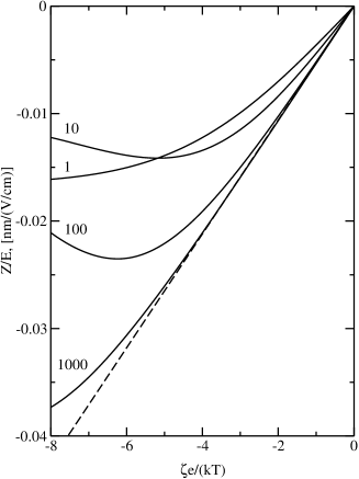
Figure 2: The ratio of the displacement $Z$ (nm) to the electric field strength $E$ (V cm^-1) as a function of the scaled $\zeta$-potential $\zeta e/(kT)$ for various scaled reciprocal double-layer thicknesses $\kappa a=1$, 10, 100 and 1000: NaCl at $T=298$ K; $a=500$ nm; ${\ell}=5$ nm; ${\cal E}=1$ kPa; $\nu=1/2$. Note that the displacement is inversely proportional to Young’s modulus ${\cal E}$. The dashed-line is the boundary-layer theory [Eqn. (39)].

Figure 3 shows $Z/E$ under the same conditions as in figure 2, but now as a function of the scaled reciprocal double-layer thickness $\kappa a$, with each curve corresponding to a constant $\zeta$-potential. The displacement is clearly a weak function of $\kappa a$, particularly when $|\zeta|$ is small, and, as expected from figure 2, a much stronger function of $\zeta$. Clearly, this way of presenting the results emphasizes the large values of $\kappa a$ required for the boundary-layer theory to be accurate.

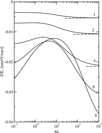
Figure 3: The ratio of the displacement $Z$ (nm) to the electric field strength $E$ (V cm^-1) as a function of the scaled reciprocal double-layer thickness $\kappa a$ for various scaled $\zeta$-potentials $-\zeta e/(kT)=1$, 2, 4, 6 and 8: NaCl at $T=298$ K; $a=500$ nm; ${\ell}=5$ nm; ${\cal E}=1$ kPa; $\nu=1/2$. Note that the displacement is inversely proportional to Young’s modulus ${\cal E}$. The dashed-lines are the boundary-layer theory [Eqn. (39)].

Since figures 2 and 3 are presented with a fixed value of ${\ell}/a=0.01$, it remains to establish the influence of the Darcy permeability (or Brinkman screening length). Recall, the boundary-layer theory [Eqn. (39)] indicates that the displacement is independent of ${\ell}$. More generally, however, the particle displacement reflects the far-field electric-field-induced distortion of the polymer skeleton when the particle is fixed at the origin by an external force

$$\mbox{\boldmath$f$\unboldmath}^{E}=-\mbox{\boldmath$f$\unboldmath}^{d,E}-\mbox{\boldmath$f$\unboldmath}^{e,E}-\mbox{\boldmath$f$\unboldmath}^{m,E}=-(8/3)\pi Z^{E}{\cal E}\mbox{\boldmath$E$\unboldmath}.$$ (40)

Figure 4 shows how the particle displacement varies over four decades of the scaled Brinkman screening length $\kappa{\ell}$ when $\zeta e/(kT)=-6$ and $\kappa a=10^{-2}$–$10^{3}$. While there are obvious transitions when $\kappa{\ell}\sim 1$ (from plateaus where $\kappa{\ell}\rightarrow 0$ and $\infty$), the displacement is remarkably insensitive to ${\ell}$.

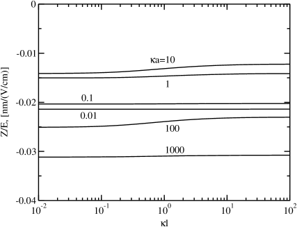
Figure 4: The ratio of the displacement $Z$ (nm) to the electric field strength $E$ (V cm^-1) as a function of the scaled Brinkman screening length $\kappa{\ell}$ with $\zeta e/(kT)=-6$ and $\kappa a=0.01$, 0.1, 1,…, 1000: KCl at $T=298$ K; $a=500$ nm; ${\cal E}=1$ kPa; $\nu=1/2$. Note that the displacement is inversely proportional to Young’s modulus ${\cal E}$.

In the next section, we identify a simple transformation that permits $Z^{E}$ and, hence, the particle displacement, to be approximated by the well-known electrophoretic mobility, which, of course, is independent of ${\ell}$. Accordingly, we write

$$\mbox{\boldmath$Z$\unboldmath}=3\zeta\epsilon_{s}\epsilon_{o}{\cal E}^{-1}f[\kappa a,\zeta e/(kT),\kappa{\ell}]\mbox{\boldmath$E$\unboldmath},$$ (41)

where the dimensionless function

$$f[\kappa a,\zeta e/(kT),\kappa{\ell}]=\frac{4\hat{Z}^{E}[\kappa a,\zeta e/(kT),\kappa{\ell}]}{9(\kappa a)^{2}\zeta e/(kT)}$$ (42)

and, to a reasonable approximation,

$$f[\kappa a,\zeta e/(kT),\kappa{\ell}]\approx f[\kappa a,\zeta e/(kT),\infty].$$ (43)

It follows that figure 2 or 3 is sufficient to span a significant range of the parameter space (strictly for negatively charged inclusions and NaCl electrolyte). Furthermore, from Eqns. (2) and (39), it is evident that $f\rightarrow 2/3$ as $\kappa a\rightarrow 0$ (with $|\zeta|<kT/e$) and $f\rightarrow 1$ as $\kappa a\rightarrow\infty$.

5.2 Connection to the electrophoretic mobility

The displacements shown in figures 2 and 3 bear a close resemblance to the electrophoretic mobility (O’Brien & White, 1978), so we present in figures 5 and 6 a scaled displacement

$$(Z/E){\cal E}e/(2\epsilon_{s}\epsilon_{o}kT)=(3/2)f[\kappa a,\zeta e/(kT),\kappa{\ell}]\zeta e/(kT)$$ (44)

for a symmetrical electrolyte (KCl) (solid lines, figure 5) and a representative asymmetric electrolyte (Ba(NO₃)₂) (figure 6). This dimensionless quantity (solid lines) has a very similar dependence on $\kappa a$ and $\zeta e/(kT)$ as the scaled electrophoretic mobility (dashed lines)

$$(U/E)3\eta e/(2\epsilon_{s}\epsilon_{o}kT)$$ (45)

presented in O’Brien and White’s well-known paper (see O’Brien & White, 1978, figures 3, 4, & 6). Here, $U$ is the electrophoretic velocity, i.e., the translational velocity acquired by a charged spherical colloid dispersed in a Newtonian electrolyte in response to a (weak) electric field $E$.

The difference between the scaled mobility and scaled displacement highlighted in figure 5 is small when $|\zeta|<kT/e$, but increases appreciably when $\kappa a\sim 1$ and $|\zeta|>3kT/e$. Note that the scaled mobility is smaller than the respective scaled displacement, because the electrophoresis problem over-estimates the convective contribution to the ion fluxes, thereby over-polarizing the diffuse double layer and, therefore, under-estimating the electrical force in the particle-displacement problem.

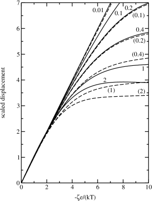
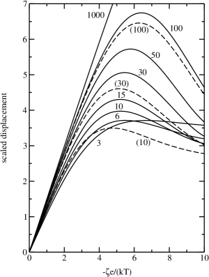
Figure 5: The scaled displacement $-(Z/E){\cal E}e/(2\epsilon_{s}\epsilon_{o}kT)$ as a function of the scaled $\zeta$-potential $-\zeta e/(kT)$ for various scaled reciprocal double-layer thicknesses $\kappa a=0.01$, 0.1, 0.2, 0.4, 1 and 2 (solid lines, left panel); and $\kappa a=3$, 6, 10, 15, 30, 50, 100 and 1000 (solid lines, right panel): KCl at $T=298$ K; $a=500$ nm; ${\ell}=5$ nm; $\nu=1/2$. Dashed lines are the scaled electrophoretic mobility $(U/E)3\eta e/(2\epsilon_{s}\epsilon_{s}kT)$ for selected values (labels in parentheses) of $\kappa a=0.01$, 0.1, 0.2, 0.4, 1 and 2 (left panel); and 10, 30 and 100 (right panel).

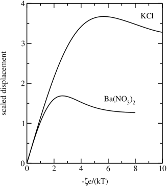
Figure 6: The scaled displacement $-(Z/E){\cal E}e/(2\epsilon_{s}\epsilon_{o}kT)$ as a function of the scaled $\zeta$-potential $-\zeta e/(kT)$ for scaled reciprocal double-layer thickness $\kappa a=5$: KCl and Ba(NO₃)₂ at $T=298$ K; $a=500$ nm; ${\ell}=5$ nm; $\nu=1/2$.

A simple but approximate relationship between $Z/E$ and $U/E$ can be established by eliminating the Darcy drag force from the fluid momentum equation [Eqn. (5)] and the polymer equation of static equilibrium [Eqn. (10)]. This produces the momentum conservation equation in the electrophoresis problem [i.e., Eqn. (5) without the Darcy drag term] with a modified ‘fluid’ velocity

$$\mbox{\boldmath$u$\unboldmath}^{\prime}=\mbox{\boldmath$u$\unboldmath}+\mbox{\boldmath$v$\unboldmath}{\cal E}/(3\eta).$$ (46)

Recall, $u$ is the fluid velocity in the polymer gel and $v$ is the displacement of the skeleton.

By setting $\mbox{\boldmath$u$\unboldmath}=\mbox{\boldmath$u$\unboldmath}^{\prime}$ in the ion conservation equation, the solution of the electrophoresis problem (involving only $\mbox{\boldmath$u$\unboldmath}^{\prime}$) over-estimates the convective ion fluxes by an $O[(v_{c}/u_{c}){\cal E}/(3\eta)]$ amount; here, $v_{c}$ and $u_{c}$ are, respectively, characteristic polymer displacement and fluid velocity scales. However, since the convective ion fluxes are $O(\mbox{Pe}_{j})$, where the Péclet numbers $\mbox{Pe}_{j}=u_{c}\kappa^{-1}/D_{j}\ll 1$, the absolute errors are small.

Note that the polymer displacement reflects a transfer of the electrical body force from the fluid to the elastic skeleton. This transfer occurs by direct coupling of the fluid and polymer (via the Darcy drag force) and through indirect coupling by the transfer of viscous stresses from the fluid to the particle, which, in turn, are transferred to the polymer via mechanical contact between the particle and polymer. Consequently, the polymer distortion must be independent of the permeability in so far as the electrical body force is constant. However, the electrically driven flow increases significantly with the permeability [either as ${\ell}$ or ${\ell}^{2}$, depending on $\kappa^{-1}$ (Hill, 2006c, a)], so the $O[(v_{c}/u_{c}){\cal E}/(3\eta)]$ errors in the ion conservation equations must diminish with increasing permeability. Accordingly, the solution of the electrophoresis problem must yield an increasingly accurate solution of the particle displacement problem as $\kappa{\ell}\rightarrow\infty$.

More quantitatively, the solution of the (E) electrophoresis problem (O’Brien & White, 1978) yields $u^{\prime}\sim\overline{C}^{E}Er^{-1}$ as $r\rightarrow\infty$. Therefore, because $v\sim Z^{E}Er^{-1}$ and $u\sim C^{E}Er^{-3}$ as $r\rightarrow\infty$, it follows from Eqn. (46) that

$$Z^{E}\rightarrow\overline{C}^{E}3\eta/{\cal E}\mbox{ as }\kappa{\ell}\rightarrow\infty\ \ (\nu=1/2).$$ (47)

Furthermore, since the electrophoretic mobility

$$M\equiv U/E=\overline{C}^{E}/\overline{C}^{U},$$ (48)

where $\overline{C}^{E}$ and $\overline{C}^{U}$ are the asymptotic coefficients associated with the far-field decay of the fluid velocity in the (E) and (U) (electrophoresis) problems (O’Brien & White, 1978), Eqns. (17), (47) and (48) give

$$\mbox{\boldmath$Z$\unboldmath}\rightarrow F(3\eta/{\cal E})M\mbox{\boldmath$E$\unboldmath}\mbox{ as }\kappa{\ell}\rightarrow\infty\ \ (\nu=1/2).$$ (49)

Note that $F=(4/3)\overline{C}^{U}/a=D_{s}/D\sim 1$ is the particle drag coefficient, which can be conveniently expressed as the ratio of the Stokes-Einstein-Sutherland diffusivity $D_{s}=kT/(6\pi\eta a)$ to the actual diffusivity $D[\kappa a,\zeta e/(kT)]\geq D_{s}$. The drag coefficient is shown in figure 7 for negatively charged colloidal spheres in a KCl electrolyte. Since $1\leq F<1.2$ and most often $1\leq F\lesssim 1.02$, the error in the particle displacement that comes from setting $F=1$ in Eqn. (49) tends to be small compared to the error arising from finite $\kappa{\ell}$.

To demonstrate the correctness of Eqn. (49), let us briefly consider a specific example where $\zeta e/(kT)=-6$ and $\kappa a=10$. From figure 4, the scaled displacements are $\approx 3.89$ and $\approx 3.42$ when $\kappa{\ell}=0.1$ and $\kappa{\ell}\rightarrow\infty$, respectively. Furthermore, from figure 5, the scaled mobility and drag coefficient are $\approx 3.36$ and $\approx 1.016$, respectively. Therefore, multiplying the scaled mobility by the drag coefficient gives $\approx 3.41$, which, as expected, compares extremely well with the value ($\approx 3.42$) obtained directly when $\kappa{\ell}\gg 1$.

In summary, we have established that the electrophoretic mobility and drag coefficient combine [as indicated in Eqn. (49)] to yield the correct limiting value of the scaled particle displacement as $\kappa{\ell}\rightarrow\infty$. Furthermore, the difference between the displacement with impenetrable and infinitely permeable polymer reflects the degree to which polymer influences convective ion transport. Finally, because polarization by convection is weak relative to electromigrative polarization and diffusive relaxation, the influence of permeability on the displacement is generally small. It should be noted, however, that Young’s modulus (or shear modulus) of the skeleton and the permeability both vary with the polymer density according to scaling laws that have been studied extensively in the polymer physics literature (e.g., de Gennes, 1979). In practice, therefore, particle displacements are expected to vary primarily with the modulus, with relatively insignificant changes due to the accompanying change in permeability.

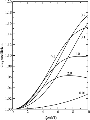
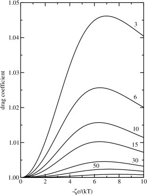
Figure 7: The drag coefficient $F=(4/3)\overline{C}^{U}/a=D_{s}/D[\kappa a,\zeta e/(kT)]$ for charged spherical colloids as a function of the scaled $\zeta$-potential $-\zeta e/(kT)$ for various scaled reciprocal double-layer thicknesses $\kappa a=0.01$, 0.1, 0.2, 0.4, 1 and 2 (left panel); and $\kappa a=3$, 6, 10, 15, 30, 50, 100 and 1000 (right panel): KCl at $T=298$ K.

6 Application to micro-rheology

As demonstrated above, dimensional particle displacements are $\lesssim 10\epsilon_{s}\epsilon_{o}kTE/(e{\cal E})$ in the experimentally accessible range of $\kappa a$ and $|\zeta|e/(kT)$. In polymer gels saturated with aqueous electrolytes at room temperature, this implies that $Z<0.17(E/{\cal E})$ nm. For example, with ${\cal E}=10$ kPa and $E=100$ V cm^-1, we find $Z<0.17$ nm, which poses a significant, but not necessarily insurmountable, experimental challenge. When ${\cal E}=0.1$ kPa, however, $Z<1.7$ nm is achieved with $E=10$ V cm^-1.

As highlighted in the introduction, passive micro-rheology also tends to be limited to complex fluids whose storage modulus is $\lesssim 1$ kPa (e.g., Schnurr et al., 1997; Chen et al., 2003, for F-actin solutions and polyacrylamide gels, and $\lambda$-DNA, respectively). For hydrogels, such conditions are realized when the cross-linking density is low (de Gennes, 1979). As our theory demonstrates, high electric field strengths ($\gtrsim 1$ kV cm^-1) and/or low elastic moduli ($\lesssim 1$ kPa) are necessary to register nanometer-scale electric-field-induced particle displacements. Accordingly, to minimize the electric field strength and, hence, avoid non-linear electrokinetic phenomena and Joule heating, we propose an experimental methodology that seeks to resolve sub-nanometer particle displacements.

In contrast to existing laser tweezers micro-rheology, where two lasers are used to simultaneously perturb and image a micron-sized tracer particle (Valentine et al., 1996; Yamaguchi et al., 2005), we envision an experiment that necessitates only an imaging laser to measure $Z/E=(4/3)(Z^{E}/a)$, which, recall, reflects physicochemical characteristics of the particle-gel interface. In practice, an optical trap and piezo-electric stage (with feed-back control) may be adopted for positioning and alignment purposes.

Very small-amplitude particle displacements induced by an oscillatory electric field may be registered by correlating the measured response $Z^{\prime}=Z-\langle Z\rangle=Z^{\prime\prime}(t)+|\hat{Z}|\cos{(\omega t+\theta)}$ with the (harmonic) electric field strength $E=|\hat{E}|\cos{(\omega t)}$. Here, $Z^{\prime\prime}(t)$ denotes the noise (adjusted to have zero mean), $|\hat{Z}|$ and $|\hat{E}|$ are the amplitudes of the (harmonic) particle displacement and electric field, $\theta$ is the phase angle, $\omega$ is the angular frequency, and $t$ is time. If the noise $Z^{\prime\prime}$ is uncorrelated with the excitation $E$, then

$$\langle Z^{\prime}E\rangle\equiv T^{-1}\int_{0}^{T}Z^{\prime}(t)E(t)\mbox{d}t\rightarrow(1/2)|\hat{Z}||\hat{E}|\cos{\theta}+O(T^{-1/2})$$ (50)

if the duration $T$ of the time series is large.

The quasi-steady particle equation of motion [Eqn. (16) with viscous drag force $-6\pi\eta^{*}a\mbox{d}\mbox{\boldmath$Z$\unboldmath}/\mbox{d}t$ (Valentine et al., 1996; Yamaguchi et al., 2005)] yields a (complex) displacement

$$\hat{Z}=\frac{\hat{E}(4/3)(Z^{E}/a)}{(1+i\omega 3\eta^{*}/{\cal E})}\ \ (\nu=1/2),$$ (51)

with amplitude and phase given by

$$|\hat{Z}|=\frac{|\hat{E}|(4/3)(Z^{E}/a)}{\sqrt{1+(\omega 3\eta^{*}/{\cal E})^{2}}}\ \mbox{ and }\ \tan{\theta}=-\omega 3\eta^{*}/{\cal E}.$$ (52)

Therefore, if the viscosity and elastic modulus are known, from a complementary macro- or micro-rheology experiment, then

$$(4/3)(Z^{E}/a)=\frac{\langle Z^{\prime}E\rangle}{(1/2)\cos{\theta}|\hat{E}|^{2}\sqrt{1+(\tan{\theta})^{2}}}.$$ (53)

Moreover, at sufficiently low frequencies (i.e., $\omega\ll{\cal E}/(3\eta^{*})$), the quasi-steady response is simply

$$(4/3)(Z^{E}/a)\approx 2\langle Z^{\prime}E\rangle/|\hat{E}|^{2}\ (\nu=1/2).$$ (54)

In this manner, it is not necessary to have explicit knowledge of the visco-elastic characteristics of the gel to directly probe the physicochemical characteristics of the particle, as characterized by $(4/3)(Z^{E}/a)$. Furthermore, as a compelling alternative to a more direct measurement of $Z/E$ to determine $(4/3)(Z^{E}/a)$, the correlation $\langle Z^{\prime}E\rangle$ may provide an effective means of dealing with the small signal-to-noise ratio expected in such an experiment.

Finally, when the frequency is higher than the reciprocal draining time [Eqn. (11)], a non-trivial extension of the quasi-steady theory is necessary to account for a compressible polymer skeleton and oscillatory relative motion of the fluid and polymer phases. Levine & Lubensky (2001a) undertook such a study for particles embedded in polymer gels without electrokinetic influences. They significantly extended the prevailing quasi-steady theory (e.g., Levine & Lubensky, 2001b), identifying the frequencies where, in particular, compressibility of the polymer skeleton influences the dynamical response. Clearly, their work provides a sound basis for advancing the present theory to elucidate dynamical electrokinetic effects in micro-rheology applications.

7 Summary

We presented a theoretical model to calculate the electric-field-induced displacement of a charged, spherical colloid embedded in an electrolyte-saturated polymer gel. The standard electrokinetic model describes electric-field-induced transport of ions and electrolyte momentum, with a Darcy-drag term that couples the electrolyte mass and momentum conservation equations (Brinkman’s equations) to a continuum equation of static equilibrium for an unbounded, incompressible, linearly elastic polymer skeleton.

The scaled particle displacement

$$(Z/E){\cal E}e/(2\epsilon_{s}\epsilon_{o}kT)$$

has a similar dependence on $\zeta e/(kT)$ and $\kappa a$ as the well-known scaled electrophoretic mobility

$$(U/E)3\eta e(2\epsilon_{s}\epsilon_{o}kT).$$

More precisely, we showed that the product of the scaled electrophoretic mobility and particle drag (friction) coefficient yields the exact scaled displacement when $\kappa{\ell}\rightarrow\infty$ (i.e., when the polymer skeleton presents zero hydrodynamic resistance to flow). However, because the particle displacement decreases only slightly as $\kappa{\ell}$ passes through $\sim 1$, when increasing from 0 to $\infty$, the scaled electrophoretic mobility provides an excellent approximation of the scaled displacement over a wide range of the experimentally accessible parameter space. Therefore, as expected from electrophoresis, the scaled displacement is linear in the $\zeta$-potential when $|\zeta|\lesssim 2kT/e$, and has distinct maximums when $|\zeta|\sim 5kT/e$. The decrease in displacement with increasing $\zeta$-potential is due to polarization and relaxation of the diffuse double layer. Evidently, polarization is dominated by electromigration, since the influence of convection, which can be completely arrested by an hydrodynamically impenetrable polymer skeleton, is extremely weak.

To help deal with the small signal-to-noise ratio expected in experiments that necessitate sub-nanometer particle displacements, we established a connection between $Z/E=(4/3)(Z^{E}/a)$, which reflects the physicochemical state of the particle-gel interface, and the correlation of the response ($Z^{\prime}$) and forcing ($E$) signals in a back-focal-plane interferometry apparatus. As a particle characterization tool, the novel micro-electrokinetic experiment we describe is analogous to classical micro-electrophoresis, with existing laser tweezer micro-rheology serving as the (complementary) analogue of dynamic light scattering.

We did not examine the stresses in the surrounding polymer. Nevertheless, our calculations provide an important first step toward future studies aimed at quantifying the micro-scale states of stress (and strain) when these soft composite materials are subjected to electric fields. Our model may be helpful for studying fracture, and it provides a means of quantitatively interpreting experiments designed to measure small electric-field-induced displacements of charged inclusions. In turn, these could be used to probe the mechanics of weak (uncharged) polymer gels at length and time scales that are beyond the reach of conventional (macroscale) rheometers.

Appendix A The force to displace a finite sized sphere embedded in a compressible elastic continuum

This appendix provides an analytical solution of the equation of static equilibrium in the absence of body forces (Darcy drag). In turn, the force required to displace (by distance $Z$) a rigid sphere (with radius $a$) embedded in an unbounded elastic continuum (with Young’s modulus ${\cal E}$ and Poisson’s ratio $\nu$) is obtained.

Substituting a solution of the form

$$\mbox{\boldmath$v$\unboldmath}=\mbox{\boldmath$v$\unboldmath}_{0}+\mbox{\boldmath$v$\unboldmath}_{1},$$ (55)

where

$$\nabla^{2}{\mbox{\boldmath$v$\unboldmath}_{0}}=\mbox{\boldmath$0$\unboldmath},$$ (56)

into the equation of static equilibrium [Eqn. (10)] gives

$$\nabla^{2}{\mbox{\boldmath$v$\unboldmath}_{1}}+\frac{1}{(1-2\nu)}\mbox{\boldmath$\nabla$\unboldmath}{[\mbox{\boldmath$\nabla$\unboldmath}\cdot{(\mbox{\boldmath$v$\unboldmath}_{0}+\mbox{\boldmath$v$\unboldmath}_{1})}]}=\mbox{\boldmath$0$\unboldmath}.$$ (57)

Taking the curl yields

$$\nabla^{2}{(\mbox{\boldmath$\nabla$\unboldmath}\times{\mbox{\boldmath$v$\unboldmath}_{1}})}=0,$$ (58)

which, with the prevailing axial symmetry, provides a scalar equation for $(\mbox{\boldmath$\nabla$\unboldmath}\times{\mbox{\boldmath$v$\unboldmath}_{1}})\cdot\mbox{\boldmath$e$\unboldmath}_{\phi}$. Since $\mbox{\boldmath$\nabla$\unboldmath}\times{\mbox{\boldmath$v$\unboldmath}_{1}}$ is an harmonic pseudo vector, symmetry and linearity yield a non-zero decaying solution $\mbox{\boldmath$\nabla$\unboldmath}\times{\mbox{\boldmath$v$\unboldmath}_{1}}\sim\mbox{\boldmath$Z$\unboldmath}\times\mbox{\boldmath$\nabla$\unboldmath}{r^{-1}}$. It follows that $\mbox{\boldmath$v$\unboldmath}_{1}\sim\mbox{\boldmath$Z$\unboldmath}r^{-1}$, which is harmonic and, hence, can be attributed to $\mbox{\boldmath$v$\unboldmath}_{0}$. Accordingly, the only non-harmonic contribution to $\mbox{\boldmath$v$\unboldmath}_{1}$ is irrotational ($\mbox{\boldmath$\nabla$\unboldmath}\times{\mbox{\boldmath$v$\unboldmath}_{1}}=\mbox{\boldmath$0$\unboldmath}$) and, hence,

$$\mbox{\boldmath$v$\unboldmath}_{1}=\mbox{\boldmath$\nabla$\unboldmath}{\phi},$$ (59)

where $\phi$ is a scalar function of position. Substituting this into Eqn. (57) gives

$$\mbox{\boldmath$\nabla$\unboldmath}{[\mbox{\boldmath$\nabla$\unboldmath}\cdot{\mbox{\boldmath$v$\unboldmath}_{0}}+2(1-\nu)\nabla^{2}{\phi}]}=\mbox{\boldmath$0$\unboldmath},$$ (60)

so

$$\mbox{\boldmath$\nabla$\unboldmath}\cdot{\mbox{\boldmath$v$\unboldmath}_{0}}+2(1-\nu)\nabla^{2}{\phi}=0.$$ (61)

Again, symmetry and linearity considerations yield the general decaying solution

$$\mbox{\boldmath$v$\unboldmath}_{0}=c_{0}\mbox{\boldmath$Z$\unboldmath}+c_{1}\mbox{\boldmath$Z$\unboldmath}r^{-1}+c_{2}(\mbox{\boldmath$Z$\unboldmath}\cdot\mbox{\boldmath$\nabla$\unboldmath})\mbox{\boldmath$\nabla$\unboldmath}(r^{-1}).$$ (62)

It follows that

$$\mbox{\boldmath$\nabla$\unboldmath}\cdot{\mbox{\boldmath$v$\unboldmath}_{0}}=c_{1}\mbox{\boldmath$Z$\unboldmath}\cdot\mbox{\boldmath$\nabla$\unboldmath}(r^{-1})\ \ (=-c_{1}\mbox{\boldmath$Z$\unboldmath}\cdot\mbox{\boldmath$e$\unboldmath}_{r}r^{-2})$$ (63)

and, hence,

$$\nabla^{2}{\phi}=-\frac{c_{1}\mbox{\boldmath$Z$\unboldmath}\cdot\mbox{\boldmath$\nabla$\unboldmath}(r^{-1})}{2(1-\nu)}.$$ (64)

Note that $\nabla^{2}{\psi}=r^{-1}$ has the solution $\psi=r/2$, so writing Eqn. (64) as

$$\nabla^{2}{\phi}=-\frac{c_{1}\mbox{\boldmath$Z$\unboldmath}\cdot\mbox{\boldmath$\nabla$\unboldmath}{(\nabla^{2}{\psi})}}{2(1-\nu)}$$ (65)

requires

$$\phi=-\frac{c_{1}\mbox{\boldmath$Z$\unboldmath}\cdot\mbox{\boldmath$e$\unboldmath}_{r}}{4(1-\nu)}$$ (66)

and, hence,

$$\mbox{\boldmath$v$\unboldmath}_{1}=\mbox{\boldmath$\nabla$\unboldmath}{\phi}=-\frac{c_{1}}{4r(1-\nu)}[\mbox{\boldmath$Z$\unboldmath}-(\mbox{\boldmath$Z$\unboldmath}\cdot\mbox{\boldmath$e$\unboldmath}_{r})\mbox{\boldmath$e$\unboldmath}_{r}].$$ (67)

Finally, the complete displacement field is

$$\mbox{\boldmath$v$\unboldmath}=c_{0}\mbox{\boldmath$Z$\unboldmath}+\frac{c_{1}}{r}\mbox{\boldmath$Z$\unboldmath}-\frac{c_{1}}{4r(1-\nu)}[\mbox{\boldmath$Z$\unboldmath}-(\mbox{\boldmath$Z$\unboldmath}\cdot\mbox{\boldmath$e$\unboldmath}_{r})\mbox{\boldmath$e$\unboldmath}_{r}]+\frac{c_{2}}{r^{3}}[3(\mbox{\boldmath$Z$\unboldmath}\cdot\mbox{\boldmath$e$\unboldmath}_{r})\mbox{\boldmath$e$\unboldmath}_{r}-\mbox{\boldmath$Z$\unboldmath}],$$ (68)

where the scalar constants $c_{0}$, $c_{1}$ and $c_{2}$ must be chosen to satisfy the boundary conditions.

A.1 No-slip boundary condition

If, for example, $\mbox{\boldmath$v$\unboldmath}\rightarrow-\mbox{\boldmath$Z$\unboldmath}$ as $r\rightarrow\infty$ and $\mbox{\boldmath$v$\unboldmath}=\mbox{\boldmath$0$\unboldmath}$ at $r=a$ (fixed), then $c_{0}=-1$ and

$$\mbox{\boldmath$0$\unboldmath}=-\mbox{\boldmath$Z$\unboldmath}+\frac{c_{1}}{a}\mbox{\boldmath$Z$\unboldmath}+\frac{c_{2}}{a^{3}}[3(\mbox{\boldmath$Z$\unboldmath}\cdot\mbox{\boldmath$e$\unboldmath}_{r})\mbox{\boldmath$e$\unboldmath}_{r}-\mbox{\boldmath$Z$\unboldmath}]-\frac{c_{1}}{4a(1-\nu)}[\mbox{\boldmath$Z$\unboldmath}-(\mbox{\boldmath$Z$\unboldmath}\cdot\mbox{\boldmath$e$\unboldmath}_{r})\mbox{\boldmath$e$\unboldmath}_{r}],$$ (69)

which requires

$$c_{1}=\frac{6(1-\nu)a}{(5-6\nu)}\mbox{ and }c_{2}=\frac{a^{3}}{2(6\nu-5)}.$$ (70)

The mechanical-contact force on the inclusion is therefore

$$\mbox{\boldmath$f$\unboldmath}^{m}=\int_{r=a}\mbox{\boldmath$\sigma$\unboldmath}\cdot\hat{\mbox{\boldmath$n$\unboldmath}}\mbox{d}A=-\frac{2\pi{\cal E}c_{1}\mbox{\boldmath$Z$\unboldmath}}{(1+\nu)}=-\frac{12\pi{\cal E}a\mbox{\boldmath$Z$\unboldmath}(1-\nu)}{(5-6\nu)(1+\nu)}.$$ (71)

Note that the displacement field can be rewritten in terms of the force, so the Green’s function

$$\mbox{\boldmath$G$\unboldmath}=\frac{(1+\nu)}{8\pi{\cal E}(1-\nu)r}[(3-4\nu)\mbox{\boldmath$\delta$\unboldmath}+\mbox{\boldmath$e$\unboldmath}_{r}\mbox{\boldmath$e$\unboldmath}_{r}]$$ (72)

is obtained by changing reference frames ($\mbox{\boldmath$v$\unboldmath}=\mbox{\boldmath$Z$\unboldmath}$ at $r=a$, and $\mbox{\boldmath$v$\unboldmath}\rightarrow\mbox{\boldmath$0$\unboldmath}$ as $r\rightarrow\infty$) and letting $a\rightarrow 0$.

A.2 Slip boundary condition

Again, if $\mbox{\boldmath$v$\unboldmath}\rightarrow-\mbox{\boldmath$Z$\unboldmath}$ as $r\rightarrow\infty$, but $\mbox{\boldmath$v$\unboldmath}\cdot\mbox{\boldmath$e$\unboldmath}_{r}=0$ at $r=a$ (zero radial displacement) and $\mbox{\boldmath$\sigma$\unboldmath}\cdot\mbox{\boldmath$e$\unboldmath}_{r}-(\mbox{\boldmath$\sigma$\unboldmath}\cdot\mbox{\boldmath$e$\unboldmath}_{r})\cdot\mbox{\boldmath$e$\unboldmath}_{r}\mbox{\boldmath$e$\unboldmath}_{r}=\mbox{\boldmath$0$\unboldmath}$ at $r=a$ (zero tangential stress), then $c_{0}=-1$, and

$$c_{1}=\frac{6(1-\nu)a}{(7-8\nu)}\mbox{ and }c_{2}=\frac{(1-2\nu)a^{3}}{2(7-8\nu)}.$$ (73)

The mechanical-contact force (on the inclusion) is then

$$\mbox{\boldmath$f$\unboldmath}^{m}=-\frac{2\pi{\cal E}c_{1}\mbox{\boldmath$Z$\unboldmath}}{(1+\nu)}=-\frac{12\pi{\cal E}a\mbox{\boldmath$Z$\unboldmath}(1-\nu)}{(7-8\nu)(1+\nu)}.$$ (74)

Appendix B The leading-order isotropic stress for an incompressible elastic continuum

Writing the displacement field as

$$\mbox{\boldmath$v$\unboldmath}=\mbox{\boldmath$v$\unboldmath}_{0}+\epsilon\mbox{\boldmath$v$\unboldmath}_{1}+\epsilon^{2}\mbox{\boldmath$v$\unboldmath}_{2}+...,$$ (75)

where $\epsilon=(1-2\nu)\ll 1$, substituting this into the equation of static equilibrium

$$\nabla^{2}{\mbox{\boldmath$v$\unboldmath}}+\frac{1}{\epsilon}\mbox{\boldmath$\nabla$\unboldmath}{(\mbox{\boldmath$\nabla$\unboldmath}\cdot{\mbox{\boldmath$v$\unboldmath}})}=-(\eta/{\ell}^{2})\mbox{\boldmath$u$\unboldmath}\frac{(3-\epsilon)}{{\cal E}},$$ (76)

and collecting terms of like order in $\epsilon$ gives at $O(1)$:

$$\mbox{\boldmath$\nabla$\unboldmath}{(\mbox{\boldmath$\nabla$\unboldmath}\cdot{\mbox{\boldmath$v$\unboldmath}_{0}})}=\mbox{\boldmath$0$\unboldmath};$$ (77)

at $O(\epsilon)$

$$\nabla^{2}\mbox{\boldmath$v$\unboldmath}_{0}+\mbox{\boldmath$\nabla$\unboldmath}{(\mbox{\boldmath$\nabla$\unboldmath}\cdot{\mbox{\boldmath$v$\unboldmath}_{1}})}=-(\eta/{\ell}^{2})\mbox{\boldmath$u$\unboldmath}\frac{3}{{\cal E}};$$ (78)

at $O(\epsilon^{2})$

$$\nabla^{2}{\mbox{\boldmath$v$\unboldmath}_{1}}+\mbox{\boldmath$\nabla$\unboldmath}{(\mbox{\boldmath$\nabla$\unboldmath}\cdot{\mbox{\boldmath$v$\unboldmath}_{2}})}=(\eta/{\ell}^{2})\mbox{\boldmath$u$\unboldmath}\frac{1}{{\cal E}};$$ (79)

and at $O(\epsilon^{3})$

$$\nabla^{2}{\mbox{\boldmath$v$\unboldmath}_{2}}+\mbox{\boldmath$\nabla$\unboldmath}{(\mbox{\boldmath$\nabla$\unboldmath}\cdot{\mbox{\boldmath$v$\unboldmath}_{3}})}=\mbox{\boldmath$0$\unboldmath}.$$ (80)

Note that, if $u$ and $\mbox{\boldmath$v$\unboldmath}_{0}$ are both divergence-free, then $\mbox{\boldmath$\nabla$\unboldmath}\cdot{\mbox{\boldmath$v$\unboldmath}_{1}}$, $\mbox{\boldmath$\nabla$\unboldmath}\cdot{\mbox{\boldmath$v$\unboldmath}_{2}}$, etc., all satisfy Laplace’s equation with general solution, e.g., $\mbox{\boldmath$\nabla$\unboldmath}\cdot{\mbox{\boldmath$v$\unboldmath}_{1}}=a_{1}+b_{1}\mbox{\boldmath$E$\unboldmath}\cdot\mbox{\boldmath$\nabla$\unboldmath}{r^{-1}}$.

Because the leading contribution to the displacement $\mbox{\boldmath$v$\unboldmath}_{0}$ is divergence-free [Eqn. (77)], it can be written

$$\mbox{\boldmath$v$\unboldmath}_{0}=\mbox{\boldmath$\nabla$\unboldmath}\times\mbox{\boldmath$\nabla$\unboldmath}\times g(r)\mbox{\boldmath$E$\unboldmath}.$$ (81)

Substituting this into the curl of Eqn. (78) gives

$$\frac{\mbox{d}}{\mbox{d}r}\nabla^{2}\nabla^{2}g+\frac{3\eta}{{\cal E}{\ell}^{2}}\frac{\mbox{d}}{\mbox{d}r}\nabla^{2}f=0,$$ (82)

where

$$\nabla^{2}=\frac{1}{r^{2}}\frac{\mbox{d}}{\mbox{d}r}(r^{2}\frac{\mbox{d}}{\mbox{d}r})$$ (83)

and $f(r)$ is known. Clearly, the solution is independent of $\mbox{\boldmath$v$\unboldmath}_{1}$. Note, however, that $\mbox{\boldmath$v$\unboldmath}_{1}$ contributes to the leading-order stress,

$$\mbox{\boldmath$\sigma$\unboldmath}_{0}=\frac{2{\cal E}}{3}[\mbox{\boldmath$e$\unboldmath}_{0}+\frac{1}{2}(\mbox{\boldmath$\nabla$\unboldmath}\cdot{\mbox{\boldmath$v$\unboldmath}_{1}})\mbox{\boldmath$\delta$\unboldmath}],$$ (84)

where $\mbox{\boldmath$e$\unboldmath}_{0}=(1/2)[\mbox{\boldmath$\nabla$\unboldmath}{\mbox{\boldmath$v$\unboldmath}_{0}}+(\mbox{\boldmath$\nabla$\unboldmath}{\mbox{\boldmath$v$\unboldmath}_{0}})^{T}]$. It follows that the leading contribution to the integral of the surface traction is

$$\mbox{\boldmath$f$\unboldmath}^{\prime}_{0}=\frac{{\cal E}}{3}\int_{r\rightarrow\infty}[\mbox{\boldmath$\nabla$\unboldmath}{\mbox{\boldmath$v$\unboldmath}_{0}}+(\mbox{\boldmath$\nabla$\unboldmath}{\mbox{\boldmath$v$\unboldmath}_{0}})^{T}+(\mbox{\boldmath$\nabla$\unboldmath}\cdot{\mbox{\boldmath$v$\unboldmath}_{1}})\mbox{\boldmath$\delta$\unboldmath}]\cdot\mbox{\boldmath$e$\unboldmath}_{r}\mbox{d}A,$$ (85)

where [Eqn. (78)]

$$\mbox{\boldmath$\nabla$\unboldmath}\cdot{\mbox{\boldmath$v$\unboldmath}_{1}}=-\int_{\infty}^{r}[(\eta/{\ell}^{2})\mbox{\boldmath$u$\unboldmath}\frac{3}{{\cal E}}+\nabla^{2}\mbox{\boldmath$v$\unboldmath}_{0}]\cdot\mbox{\boldmath$e$\unboldmath}_{r}\mbox{d}r^{\prime}.$$ (86)

Note that only the far-field decays of $u$ and $\mbox{\boldmath$v$\unboldmath}_{0}$ are necessary to evaluate this integral when $r\rightarrow\infty$. Recall,

$$\mbox{\boldmath$u$\unboldmath}\rightarrow-2C^{E}r^{-3}(\mbox{\boldmath$E$\unboldmath}\cdot\mbox{\boldmath$e$\unboldmath}_{r})\mbox{\boldmath$e$\unboldmath}_{r}-C^{E}r^{-3}(\mbox{\boldmath$E$\unboldmath}\cdot\mbox{\boldmath$e$\unboldmath}_{\theta})\mbox{\boldmath$e$\unboldmath}_{\theta}\mbox{ as }r\rightarrow\infty,$$ (87)

so

$$\mbox{\boldmath$\nabla$\unboldmath}\cdot{\mbox{\boldmath$v$\unboldmath}_{1}}\rightarrow[2Z^{E}-(\eta/{\ell}^{2})\frac{3}{{\cal E}}C^{E}]r^{-2}(\mbox{\boldmath$E$\unboldmath}\cdot\mbox{\boldmath$e$\unboldmath}_{r})\mbox{ as }r\rightarrow\infty$$ (88)

and, hence,

$$\mbox{\boldmath$f$\unboldmath}^{\prime}_{0} = \frac{{\cal E}}{3}\int_{r\rightarrow\infty}\left[\left(\frac{\partial v_{0,i}}{\partial x_{j}}+\frac{\partial v_{0,j}}{\partial x_{i}}\right)+\frac{\partial v_{1,k}}{\partial x_{k}}\delta_{ij}\right]e_{r,j}\mbox{d}A$$ (89)

$$= {\cal E}(16/9)\pi Z^{E}\mbox{\boldmath$E$\unboldmath}+{\cal E}(8/9)\pi Z^{E}\mbox{\boldmath$E$\unboldmath}-(4/3)\pi(\eta/{\ell}^{2})C^{E}\mbox{\boldmath$E$\unboldmath}$$

$$= (8/3)\pi Z^{E}{\cal E}\mbox{\boldmath$E$\unboldmath}-(4/3)\pi(\eta/{\ell}^{2})C^{E}\mbox{\boldmath$E$\unboldmath}$$

Finally, adding the volume integral [$-(8/3)\pi(\eta/{\ell}^{2})C^{E}\mbox{\boldmath$E$\unboldmath}$] gives the net mechanical-contact force acting on the inclusion,

$$\mbox{\boldmath$f$\unboldmath}^{m,E}=(8/3)\pi Z^{E}{\cal E}\mbox{\boldmath$E$\unboldmath}-4\pi(\eta/{\ell}^{2})C^{E}\mbox{\boldmath$E$\unboldmath}.$$ (90)