Camouflaged galactic CMB foregrounds: total and polarized contributions of the kinetic Sunyaev Zeldovich effect

Abstract

We consider the role of the galactic kinetic Sunyaev Zeldovich (SZ) effect as a CMB foreground. While the galactic thermal Sunyaev Zeldovich effect has previously been studied and discarded as a potential CMB foreground, we find that the kinetic SZ effect is dominant in the galactic case. We analyse the detectability of the kinetic SZ effect by means of an optimally matched filter technique applied to a simulation of an ideal observation. We obtain no detection, getting a S/N ratio of 0.1, thereby demonstrating that the kinetic SZ effect can also safely be ignored as a CMB foreground. However we provide maps of the expected signal for inclusion in future high precision data processing. Furthermore, we rule out the significant contamination of the polarised CMB signal by second scattering of galactic kinetic Sunyaev-Zeldovich photons, since we show that the scattering of the CMB quadrupole photons by galactic electrons is a stronger effect than the Sunyaev Zeldovich second scattering, and has already been shown to produce no significant polarised contamination. We confirm the latter assessment also by means of an optimally matched filter.

1 Introduction

The role of the Sunyaev Zeldovich effect (hereafter SZ) as a CMB foreground has been widely studied for clusters of galaxies (see for example Sunyaev & Zeldovich (1972), Sunyaev & Zeldovich (1980), Birkinshaw (1999), Dolag et al. (2005) and Schäfer et al. (2006)). Due to the high cluster temperatures the relevant effect in these cases is the thermal SZ effect (hereafter tSZ), while the kinetic SZ effect (hereafter kSZ) is secondary. In this work we study the galactic SZ effect. The relevance of the tSZ effect as a galactic foreground has been ruled out by previous studies (see e.g. Hinshaw et al., 2007, also section 2.1.1). As we will show, however, the kSZ effect makes a significantly higher contribution. This is confirmed by an independent galactic kinetic SZ effect simulation made by Hajian et al. (2007), with whose results ours agree. Even though the galactic kSZ effect is more significant than the tSZ effect, we demonstrate by means of the optimally matched filter technique that it is still not a significant CMB foreground.

We extend our search by also investigating whether the second scattering of galactic kSZ effect photons could present a significant CMB polarisation foreground. The strength of the the polarised signal due to Thomson scattering by galactic electrons is determined by the intensity of the incident quadrupole radiation in the rest frame of the electron. Hence we assess the importance of a polarised foreground by the intensity of the incident quadrupole radiation source.

We will show, that the polarisation signal due to the intrinsic CMB quadrupole is far more significant than that caused by secondary scattering of the kSZ induced quadrupole. In addition we also examined the relevance of the CMB quadrupole induced by the mildly relativistic motion of the galaxy in the CMB rest-frame. This effect, however, is known to be an order of magnitude smaller than the intrinsic CMB quadrupole (Hinshaw et al., 2007) hence, although it is slightly more relevant for polarisation production than the kSZ quadrupole, also negligible. The CMB quadrupole induced polarisation by galactic electrons has been shown to be an insignificant CMB polarisation foreground (Hirata et al., 2005). We confirm this result in sec. 4.2, where we demonstrate by means of a matched filter that no galactic signal can be detected even assuming an idealised experiment. Hence polarisation contributions due to the weaker galactic kSZ effect can safely be ignored as CMB polarisation foreground.

The structure of the paper is the following. In section 2.1 we give a brief description of the SZ effect, while in section 2.2 we describe the Thomson scattering theory and check for the relevance of the kSZ effect polarisation signal. Section 3 describes our simulation of the galactic SZ effect and the polarised Thomson scattering emission. In Section 4 we describe our attempt to measure the SZ and polarised Thomson scattering signature in our simulations. We draw conclusions in Section 5 and discuss how both the kSZ and the polarised Thomson signal can be ignored as CMB foregrounds.

2 The Sunyaev-Zeldovich effect

Here we present a brief theoretical introduction to the SZ effect and perform an order-of-magnitude estimate of the galactic tSZ and the kSZ effects as a first step toward investigating their importance as CMB foregrounds. We do also check whether any relevant contamination of the CMB polarisation signal due to the galactic kSZ effect is expected.

2.1 Basics

The SZ effect is a distortion of the CMB signal caused by the scattering of the CMB photons on moving free electrons (see Sunyaev & Zeldovich, 1972, 1980). There are two components of the SZ effect: the thermal SZ effect due to the electron thermal velocities and the kinetic SZ effect caused by the bulk motion of electrons in the CMB rest frame. The CMB spectrum distorted by the Compton scattering is given by

$$I(x) = I_{CMB}(x)+\delta I_{tSZ}(x)+\delta I_{kSZ}(x)$$

$$= i_{0}[i(x)+g(x)y-h(x)\overline{\tau\beta}],$$

where $x=h\nu/(kT)$ is the dimensionless frequency. The CMB blackbody spectrum is

$$I_{CMB}(x)=i_{0}\,i(x),$$ (2)

with normalisation factor $i_{0}=2(kT_{cmb})^{3}/(hc)^{2}$ and spectral shape $i(x)={x^{3}}/(e^{x}-1)$. The second term on the right hand side of Eq. 2.1 describes the tSZ effect. This effect has a spectral shape given by

$$g(x)=\frac{x^{4}e^{x}}{(e^{x}-1)^{2}}\left(x\frac{e^{x}+1}{e^{x}-1}-4\right)\;,$$ (3)

and amplitude given by the Comptonization parameter for a given line-of-sight (LOS),

$$y=\frac{\sigma_{T}}{m_{e}c^{2}}\int dl\,n_{e}(l)\,kT_{e}(l).$$ (4)

The last term on the right hand side of Eq. 2.1 represents the kSZ effect. It has the spectral shape

$$h(x)=\frac{x^{4}e^{x}}{(e^{x}-1)^{2}}$$ (5)

and depends on the LOS integral

$$\overline{\tau\beta}=\sigma_{T}\int dl\,n_{e}(l)\,\beta(l).$$ (6)

Here $\beta$ is the velocity component along the LOS in units of the speed of light.

It is common practice to display CMB measurements in terms of temperature distortion maps. This is specially convenient for the kSZ effect, which can be interpreted as a frequency independent change to the original CMB temperature. The spectral distortions introduced by the kSZ effect are

$$I(x^{\prime})\simeq I(x)+\left(\frac{\partial I}{\partial x^{\prime}}\right)_{x^{\prime}=x}\!\!\!\!\!\!(x^{\prime}-x)=i_{0}\left(i(x)-h(x)\frac{\delta T}{T_{CMB}}\right)\;,$$ (7)

and therefore identical to spectral distortions generated by a temperature change, to first order. Here $x^{\prime}=\frac{h\nu}{kT^{\prime}}$, where $T^{\prime}=T_{CMB}+\delta T$ and $\delta T\ll T_{CMB}$. Comparing Eq. 2.1 and 7 suggest the identification $\overline{\tau\beta}=\delta T_{kSZ}/T_{CMB}$. In contrast, the tSZ spectral distortions cannot be described by a simple frequency-independent temperature change. However, for our galaxy the kSZ effect dominates by orders of magnitude over the tSZ effect, as we show in the following.

2.1.1 Order of magnitude estimate of the galactic thermal SZ effect

Previous works have ruled out the relevance of the thermal SZ effect as a foreground for the CMB (see Hinshaw et al., 2007). They estimate $y\simeq 2\times 10^{-8}$ by assuming a maximal temperature, density and LOS distance in Eq. 4. Thus they argue that the SZ effect can safely be ignored as a diffuse contaminating foreground signal. Indeed the galactic tSZ effect would produce a variation in temperature about three orders of magnitude smaller than the CMB primary anisotropies, at most.

2.1.2 Order of magnitude estimate of the galactic kinematic SZ effect

We will now attempt an estimate on the kSZ signal strength. The variation in temperature due to the kSZ (in the CMB rest-frame) is given by $\delta T/T_{CMB}=\overline{\tau\beta}$ which is a function of the thermal electron density and the LOS components of the electron velocities in the CMB rest-frame (Eq. 6). As a rough estimate, we consider a homogeneous gas distribution with electron density $n_{e}\sim 0.1{\rm cm}^{-3}$ (Cordes & Lazio, 2002), and a constant velocity of $371{\rm km/s}$ (see Fixsen et al., 1996) all along the LOS, with a length $L=20\,{\rm kpc}$, through the galactic plane. Hence,

$$\overline{\tau\beta}=\delta T_{kSZ}/T_{CMB}\sim\sigma_{T}\,L\,n_{e}\,\beta\sim 4\cdot 10^{-6}.$$

This toy scenario portrays how large the kSZ effect amplitude could maximally be in the direction of the galactic plane. Though still smaller than the CMB anisotropy signal, it is significantly greater than the thermal SZ effect (about two orders of magnitude). This motivates us to undertake a more precise analysis of this phenomenon by constructing a synthetic map of the galactic kSZ effect (see sec. 3.2) and to check whether it can be a non-negligible CMB foreground (see sec. 4).

2.2 Polarisation due to Thomson scattering

Polarisation due to Thomson scattering depends only on the quadrupole of the incoming radiation as is briefly demonstrated in the following.

The Q and U Stokes parameters due to Thomson scattering for each LOS are computed for a local coordinate system whose xy-plane is orthogonal to the LOS and whose z-direction points to the observer. To consistently compute the Stokes parameters for all directions on the sky we adopt the convention where the x-axis points in negative $\hat{\phi}^{\prime}$ and the y-axis in negative $\hat{\theta}^{\prime}$ direction of the observer-centric coordinate system whose $\rm{x^{\prime}}$ axis points towards the galactic centre while the $\rm{z^{\prime}}$ axis points towards the galactic north pole. Assuming the usual $\theta$ and $\phi$ angles for the local coordinate system we have

$$Q=\frac{3\sigma_{T}}{16\pi}\int dl\,n_{e}(l)\int d\Omega\,\sin^{2}\theta\,\cos 2\phi\,I(\theta,\phi,l),$$ (8)

$$U=\frac{3\sigma_{T}}{16\pi}\int dl\,n_{e}(l)\int d\Omega\,\sin^{2}\theta\,\sin 2\phi\,I(\theta,\phi,l).$$ (9)

The terms $\sin^{2}\theta\,\cos 2\phi=\sqrt{8\pi/15}\left(Y_{2}^{2}(\theta,\phi)+Y_{2}^{-2}(\theta,\phi)\right)$ and $\sin^{2}\theta\,\sin 2\phi=-i\sqrt{8\pi/15}\left(Y_{2}^{2}(\theta,\phi)-Y_{2}^{-2}(\theta,\phi)\right)$ are linear combinations of l=2 spherical harmonics, i.e. the quadrupole (here spherical harmonics are denoted by $Y_{l}^{m}(\theta,\phi)$). Hence only the quadrupole part of $I(\theta,\phi)$ survives the integration over the whole sphere:

$$\int d\Omega\,\sin^{2}\theta\,\cos 2\phi\,I(\theta,\phi) = \sqrt{\frac{8\pi}{15}}\left(a_{22}+a_{2-2}\right)$$ (10)

$$= \sqrt{\frac{32\pi}{15}}{\rm Re}\,a_{22}$$

and similarly

$$\int d\Omega\,\sin^{2}\theta\,\sin 2\phi\,I(\theta,\phi) = -i\sqrt{\frac{8\pi}{15}}\left(a_{22}-a_{2-2}\right)$$ (11)

$$= \sqrt{\frac{32\pi}{15}}{\rm Im}\,a_{22}.$$

Here, the $a_{lm}$ are the spherical harmonic coefficients. We have made use of the property $a_{l\,-m}=-1^{m}a_{lm}^{*}$ of the real valued brightness distribution, with the asterix denoting complex conjugation.

2.2.1 Estimating the relevance of the polarised signal

Here, we asses the typical strength of the polarisation signal caused by second scattering of the kSZ photons. To do so we compare it to other possible sources of polarised radiation. In order to identify the dominant polarisation signal we only have to find the strongest quadrupole source.

Table 1 lists the total power of all possibly relevant quadrupole sources. Notice that other foregrounds like synchrotron or dust emission present even stronger quadrupoles, however, since they have frequency dependent brightness temperatures, they can, in principle, be removed. We see that the CMB quadrupole is by far the most significant contribution. The Doppler quadrupole due to Earths motion in the CMB rest-frame is negligible, while the quadrupole due to second scattering of the kSZ effect is even smaller.

We first perform an order of magnitude estimate to obtain the upper limit for the polarised signal due to the scattering of the CMB quadrupole by galactic thermal electrons:

We refer to the CMB power spectrum given by Hinshaw et al. (2007). In their table 7, they display the quantity $\Delta T_{2}^{2}=211\mu K^{2}$. It is given by $\Delta T_{l}^{2}=l(l+1)C_{l}/(2\pi)$, and $C_{l}=1/(2l+1)\sum_{m=-l}^{l}|{a_{lm}}|^{2}$. For a rough upper limit estimate, we assume all quadrupole power to be concentrated on only the real part of $a_{22}=\sqrt{5C_{2}}$. Assuming a homogeneous thermal electron number density $n_{e}\sim 0.1\,{\rm cm^{-3}}$ (again following Cordes & Lazio, 2002, as in section 2.1.2) along a LOS of $L\sim 20\,{\rm kpc}$ (say towards the galactic centre) we get,

$$Q = \sigma_{T}\sqrt{\frac{3}{40\pi}}L\,n_{e}\,{\rm Re}\,a_{22}\simeq 2\cdot 10^{-2}\,{\rm\mu K}.$$ (12)

The polarised CMB intrinsic anisotropies have maximum amplitudes of $\sim 10\%$ of the total CMB anisotropies whose maxima are typically around a few ${\rm 100\mu K}\;$ (see figure 15 of Page et al., 2007). Hence, the polarisation signal due to Thomson scattering on the galactic electrons from the CMB radiation (only a few $10^{-2}\,{\rm\mu K}$) is likely to be undetectable on any Q or U maps. The much weaker kSZ contribution (see table 1) is thus likely to be an insignificant contamination to the CMB polarisation. This is supported by detailed computations of the Thomson scattering of the CMB quadrupole by galactic electrons performed by Hirata et al. (2005). The authors verify that the galactic Thomson signal is not a significant contamination to the intrinsic CMB polarisation.

Complementary to the arguments presented in Hirata et al. (2005), in sec. 4.2 we confirm by means of the matched filter technique applied to our simulations that the signal is not detectable, consequently neither is the one due to the second scattering of kSZ photons.

Quadrupole source	$C_{2}$
CMB	$221{\rm\mu K^{2}}$
relat. Doppler effect	$3.45{\rm\mu K^{2}}$
kSZ effect	$10^{-2}{\rm\mu K^{2}}$

Table 1: Amplitude of the quadrupole moments in order of their significance. The relativistic Doppler effect quadrupole moment is calculated for $\beta\sim 1.2\cdot 10^{-3}$. The CMB quadrupole given by Hinshaw et al. (2007) includes this value (i.e. they do not attempt to subtract it from the measured value). The kSZ quadrupole moment is obtained from our simulation in sec. 3.2. Other foregrounds with frequency dependent brightness temperatures like synchrotron or dust emission are assumed to be removed.

3 Simulations

3.1 The code

We modified the Hammurabi-code originally designed for simulating galactic synchrotron emission (Waelkens et al., 2007; Enßlin et al., 2006), to calculate the LOS integral given in Eq. 6 (for the kSZ effect) and in Eq. 8 and 9 (for the polarisation due to Thomson scattering). This code uses the HEALPix pixelisation scheme (Górski et al., 2005).

3.1.1 Line-of-sight integration for the kSZ effect

The flux associated with an observation beam, whose width and shape is related to the HEALPix pixels, is calculated by taking samples of the thermal electron density and the velocity along the LOS at equal radial intervals. To compensate for the widening of the beam cross section as one moves farther away from the observer, the observation beam is, after a certain distance, split into 4 sub-beams over which we then average. Each sub-beam is again individually sampled at the same regular radial intervals as before, and split again after twice the first distance, and so forth. This avoids an under-sampling of the thermal electron density and LOS velocity at large distances from the observer.

3.1.2 Line-of-sight integration for the polarised galactic Thomson scattering

In this case only the electron density is integrated along the line of sight, however the computation is performed in an analogous manner to the previous paragraph. The resulting map is multiplied by the $a_{22}$ component after a rotational coordinate transformation for each different LOS in order to get the respective $Q$ (Eq. 8) and $U$ (Eq. 9) Stokes parameters. The computation of the proper $a_{22}$ coefficients is described in appendix B.

3.1.3 Galaxy model

Two input models are needed, a model for the thermal electron distribution and a model for the galactic rotation curve.

1. For the electrons we use the NE2001 model (see Cordes & Lazio, 2002). This model subdivides the galaxy in several large scale structure elements (thin disk, thick disk, spiral arms,…) as well as some local small scale elements such as supernovae bubbles.

2. For the galactic rotation curve we assume a constant value of $220\,{\rm km/s}$ above a galactocentric distance of $2\,{\rm kpc}$. Below this distance the velocity falls off linearly to zero while approaching the galactic centre. This is an approximation for the observed rotation curve (see e.g. Klypin et al., 2002, and references therein), which should be adequate to determine whether the galactic kSZ effect can be detected.

3.2 Constructing the kSZ map

The velocity of each point of the galaxy with respect to the CMB rest-frame is subdivided into two components. The rotation velocity of the galaxy ($\beta_{rot}$) and the position-independent translation velocity of the galaxy ($\beta_{trn}$). The first quantity is obtained from our rotation curve model. The later quantity is obtained by subtracting our solar systems galactic rotation velocity vector ($220\,{\rm km/s}$ in $l=\pi/2$ direction) from the measured total CMB frame velocity ($371{\rm km/s}$ in $l\simeq 1.47\pi$ and $b\simeq 0.27\pi$ direction, see Fixsen et al., 1996). Since the resulting $\beta$ is small($\sim 10^{-3}$), we can safely ignore relativistic effects when adding velocities.

However, relativistic effects may need to be considered for the temperature transformation. So far we obtained the $\overline{\tau\beta}=\delta T/T_{CMB}$ sky in the CMB rest-frame. The relativistic temperature transformation is given by $\delta T_{obsf}=\delta T_{cmbf}\left[\gamma\left(1+(\beta_{tot}\,\mu_{obsf})\right)\right]^{-1}$ . Here $\mu_{obsf}$ is the cosine of the angle between the opposite of the CMB frame motion direction and the LOS in the observer rest-frame and $\gamma=(1-\beta^{2})^{-1/2}$. The relativistic correction to the temperature is small, in the extreme a factor $\sim(1\pm 10^{-3})$, which can be safely ignored, leaving $\delta T_{obsf}=\delta T_{CMBf}$. Thus to obtain the kSZ map we can neglect all relativistic effects.

Finally, we obtain the kSZ map by inserting our galaxy model in Eq. 6. The resulting map is shown in figure 1. Note the local interstellar medium features of the thermal electron density model (see sec. 3.1.3). We subtracted the monopole and dipole in accordance with the standard practice of subtracting the monopole and the relativistic-Doppler-effect induced dipole from maps displaying the CMB anisotropies. Our simulations show that this has a small effect, decreasing the maximum amplitude of the map by about 20$\%$.

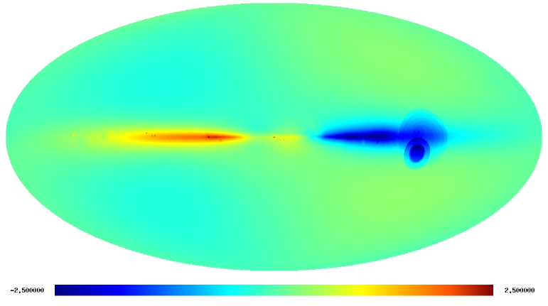
Figure 1: $\delta T=\overline{\tau\beta}\cdot T$ map in ${\rm\mu K}$. The monopole and dipole components of the map have been subtracted in analogy to what typically is done for the observations (e.g. WMAP). Our simulation shows that the maximum amplitude of the map decreases by about 20$\%$ once the kSZ dipole is subtracted. Notice the features due to over dense or under dense regions in the local interstellar medium.

The maximum amplitudes of the simulated signal are of the order of ${\rm\mu K}$, in accordance with the estimate obtained in section 2.1.2, and two orders of magnitude smaller than the CMB intrinsic anisotropies.

3.3 Constructing the polarised Thomson scattering maps

The expressions for the Q and U stokes parameters (Eqs. 8 and 9) assume that the negative z-axis of the coordinate system coincides with the LOS direction. Thus it is necessary to compute the appropriate $a_{22}$ coefficient for each direction on the sky. This is done by rotating a set of $a_{2m}$ coefficients, which are given in a certain coordinate system e.g. that in which the WMAP data are presented, to the proper coordinate system in which the negative z-axis is aligned with the LOS. The procedure for rotating $a_{lm}$ coefficients is described in detail in Varshalovich et al. (1988) and de Oliveira-Costa et al. (2004). For completeness, we reproduce our special case in the appendix B. Having performed the rotation we may apply Eqs. 10 and 11 to each position on the sky, which after performing a LOS integral of the thermal electron density, finally allow us to compute Q and U, using Eqs. 8 and 9 respectively. The resulting full sky maps are shown in figures 2 and 3. The maximum amplitudes are $\sim 10^{-3}\,{\rm\mu K}$, about one order of magnitude lower than our estimate in section 2.2. Out of the Q and U maps, the E and B mode spherical harmonic coefficients are obtained. Since most of the CMB polarisation power is in E modes, the B-modes signal of the polarised galactic Thomson scattering is more relevant as a CMB polarisation contamination than the corresponding E-mode signal. In sec. 4.2 we search for B-mode signal contamination by polarised galactic Thomson-scattering.

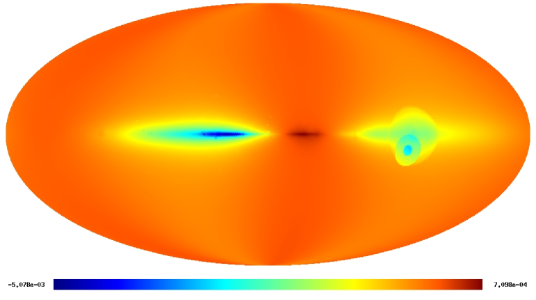
Figure 2: Stokes Q in $\rm{\mu K}$.

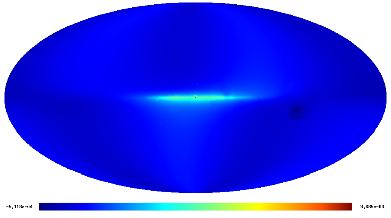
Figure 3: Stokes U in $\rm{\mu K}$.

4 Filtering

In order to estimate the feasibility of a detection of the effects discussed above, we construct and apply an optimally matched filter to simulated data, where we probe for the galactic kSZ and galactic polarised Thomson scattering signatures.

The optimal matched filter was proposed for measuring radial bulk motion of galaxy clusters through their kSZ imprint (Haehnelt & Tegmark, 1996) and subsequently found a wide range of applications in the literature, such as weak lensing and the RS effect (see e.g. Maturi et al., 2005, 2006). A scalar adaptive generalisation of the filter on the sphere was done by Schäfer et al. (2006), and later extended to allow non-azimuthally symmetric objects to be detected (McEwen et al., 2006). We use a similar approach to Schäfer et al. (2006). However, instead of convolving the CMB signal and the filter for various positions and orientations, we need only perform one convolution since we already know the position and orientation of our signal. Details are presented in the appendix A. The estimate of the maximum amplitude of the targeted signal is given by the convolution of the filter $\Psi$ with the signal $S$

$$\overline{A}=\int d\Omega\,\Psi(\theta,\phi)S(\theta,\phi),$$ (13)

while the variance is

$$\sigma^{2} = <\overline{A}>^{2}-A^{2}=\sum_{l}\sum_{m}C_{l}\left|\psi_{lm}\right|^{2}.$$ (14)

Here $\psi_{lm}$ is the spherical harmonic coefficient of the filter. The angular power spectrum of the noise ($C_{l}$) is either, in the kSZ case, the temperature angular power of the CMB plus instrumental Gaussian noise, or, in the polarised Thomson-scattering case, the B-mode angular power spectrum plus corresponding Gaussian instrumental noise. The filter is defined such that $\sigma^{2}$ is minimal while the bias $b=\langle\overline{A}\rangle-A=0$ is zero.

Figure 4: Comparing the CMB power spectrum to the simulated kSZ power spectrum. The saw like pattern for the kSZ effect power spectrum is due to the fact that even spherical harmonics are zero at the equator of the coordinate system, which in this case corresponds to the galactic plane. Hence odd modes will have more power.

4.1 Filtering on simulated data: galactic kSZ

We consider the ideal situation in which the only additional contribution to the CMB plus instrumental noise signal is the kSZ effect.

We do a simulation of the CMB sky with a sampling resolution of about $7\,{\rm arcmin}$ (corresponding to the HEALPix parameter NSIDE=512) and assume experimental characteristics expected for a Planck-like experiment, i.e. a resolution of 10 arcmin and a sensitivity of $5\,{\rm\mu K/beam}$. Given that the structures of the simulated kSZ effect are mostly on larger scales (see figure 4), the sensitivity, instead of the resolution, is the more relevant instrumental characteristic here. We generate a kSZ map with the same sampling resolution, add it to the synthetic CMB sky and then convolve the map with a one degree Gaussian kernel. This smooths the sharp borders of the simulation and also ensures that our final map is properly sampled. The result is shown in figure 5, in which no evidence of the kSZ effect is visible.

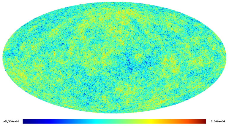
Figure 5: Simulated CMB sky contaminated by the simulated galactic kSZ effect.

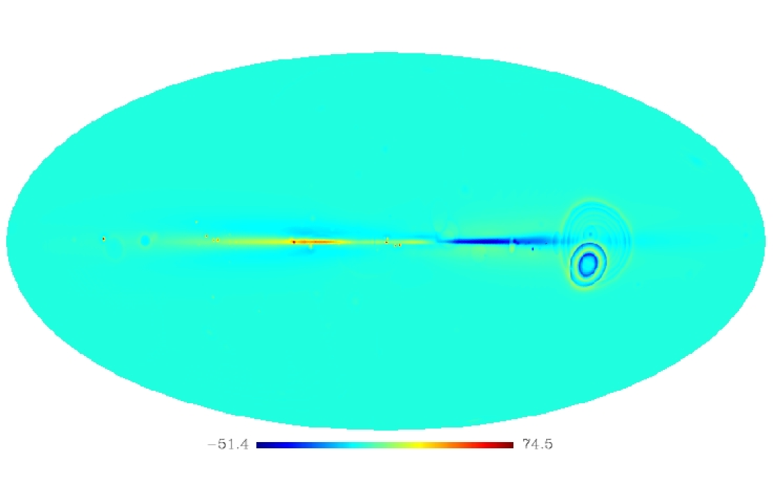
Figure 6: The optimally matched galactic kSZ filter. Note the features due to the local inter stellar medium components of the thermal electron density model (Cordes & Lazio, 2002).

As a signal template we take the same convolved kSZ map previously used in defining the data. This highly idealised approach (assuming a perfect signal template and no contamination by other Galactic emission sources) is suitable to determine the best possible filter performance.

The signal amplitude obtained by applying the filtering technique is $-10\pm 21{\rm\mu K}$, with the variance given by Eq. 14. The expected maximum amplitude of the kSZ map, the quantity we are estimating with the optimally matched filter, is $2.4{\rm\mu K}$, according to our model. Hence we have a signal-to-noise ratio of 0.1.

Although in this simulation no other foregrounds were present, no detection was possible, demonstrating that the galactic kSZ effect can be ignored as a CMB foreground.

4.2 Filtering on simulated data: the B-mode signal

The measurement of CMB B modes is the next cosmological challenge and would be very relevant for constraining inflationary models. The CMB polarised power is overwhelmingly in the E-modes, contrary the polarised galactic Thomson scattering. For this, our simulation shows a balance between the E and B-mode power on large scales, and a difference by at most one order of magnitude on smaller scales. This implies that the galactic B-mode contamination of the CMB is relatively stronger than the corresponding E-mode contamination. Therefore applying the same filtering technique as in sec. 4 we can investigate whether the polarised Thomson scattered B-mode signal is detectable and, if so, whether it is a relevant CMB foreground.

We use the predicted CMB BB power spectrum $C^{BB}_{l}$ (as given by the CAMB code, Lewis et al., 2000) for a tensor-to-scalar ratio of $10^{-5}$ (following Hirata et al., 2005), plus the instrumental noise for a sensitivity of $7.6\,{\rm\mu K/beam}$ and a resolution of $30$ arcmin (corresponding to polarisation instrumental characteristics of a Planck-like experiment), as the noise power spectrum in Eq. 24. The tensor spherical harmonic coefficients $b^{Thomson}_{lm}\rightarrow\tau_{lm}$ for the B modes of our polarised galactic Thomson-scattering simulation are used as the spherical harmonic coefficients of our template.

This analogy to the previous case is permissible since $C^{BB}_{l}$ is completely uncorrelated between each different mode (like the CMB temperature power spectrum), and the CMB B mode signal is uncorrelated with the galactic B mode signal.

We obtain an estimate of $-4\cdot 10^{-3}\pm 5.8\cdot 10^{-2}{\rm\mu K}$, against the simulated signal amplitude of $1.6\cdot 10^{-3}{\rm\mu K}$. Since the achieved signal-to-noise ratio is $\sim 0.03$, the Thomson scattering by galactic thermal electrons is a negligible contribution to the CMB polarisation signal.

5 Conclusions

We have investigated the role of the galactic kinetic Sunyaev-Zeldovich effect as a CMB foreground, both for the total and polarised emission. This was done by means of an optimally matched filter based on a model of the signal and the expected noise power spectrum. The filter returns an unbiased estimate of the peak signal amplitude and is optimal in the sense that it provides the minimum variance for such a measure.

Regarding the non-polarised kinetic Sunyaev-Zeldovich emission as a CMB foreground, we found that, although the kinetic Sunyaev-Zeldovich effect is more relevant than the thermal Sunyaev-Zeldovich effect, it is still not strong enough to be detectable by means of an optimally matched filter.

Our simulation for the kinetic Sunyaev-Zeldovich effect shows the signal to be concentrated on the galactic plane where the electron density is highest. The maximum amplitude of the simulated signal (the quantity estimated by the filtering procedure) is $2.4{\rm\mu K}$. Assuming an instrument with resolution of 10 arcmin and a sensitivity of $5\,{\rm\mu K/beam}$, we obtain a signal amplitude of $-10\pm 21{\rm\mu K}$. Hence, no kinetic Sunyaev-Zeldovich effect signature could be detected.

We further demonstrate that the secondary scattering of kinetic Sunyaev-Zeldovich photons is negligible as a polarisation source. It is a weaker effect than the polarised emission due to Thomson scattering of CMB photons by galactic electrons. Again by means of the optimally matched filter technique, we determined that the latter effect is also irrelevant even as a CMB B-mode foreground, assuming a tensor to scalar ratio of $10^{-5}$ (where most of the polarised CMB power is in E-modes, and hence the B-modes are more easily contamined). The polarised galactic Thomson-scattering signal is also concentrated on the galactic plane. The maximum amplitude of the simulated signal is $8\cdot 10^{-4}{\rm\mu K}$. Assuming a Planck-like instrument with a resolution of 30 arcmin and a sensitivity of $7.6\,{\rm\mu K/beam}$, we estimate an amplitude of $-4\cdot 10^{-3}\pm 5.8\cdot 10^{-2}{\rm\mu K}$; thus no contamination of the CMB B-mode signal is detectable.

In conclusion, galactic foregrounds due to the kinetic Sunyaev-Zeldovich effect are a certainly existing, however perfectly camouflaged contamination of the CMB. Nevertheless, it is an expected physical effect which generates 1$\%$ temperature-fluctuation amplitude corrections on large scales, and thus should be taken into account when estimating the error of precision measurements as the Planck satellite will provide.

Appendix A Filter derivation

In this section we describe how to obtain an optimally matched filter function $\Psi(\theta,\phi)=\sum_{l}\sum_{m}\psi_{lm}Y_{l}^{m}(\theta,\phi)$ for attempting to detect a non azimuthally-symmetric target signal (such as the signal due to e.g. the galactic kSZ or the B mode due to galactic Thomson scattering) in the presence of a Gaussian random noise (e.g. the sum of CMB anisotropies, total or polarised, and the instrumental noise). We used such a filtering procedure in investigations of the RS effect (Maturi et al., 2007).

Following the arguments layed out by Haehnelt & Tegmark (1996), Maturi et al. (2005) and Schäfer et al. (2006), we assume the data to be composed of the statistically homogeneous CMB anisotropies, some instrumental Gaussian random noise and the targeted signal. The expansion of the data in spherical harmonics ($Y_{l}^{m}(\theta,\phi)$) is

$$S(\theta,\phi)=\sum_{l}\sum_{m}s_{lm}Y_{l}^{m}(\theta,\phi),$$ (15)

where we model the complex coefficient $s_{lm}$ as

$$s_{lm}=A\tau_{lm}+a_{lm}.$$ (16)

We choose $A$ to be the maximum amplitude of the targeted signal, while the morphology is encoded in the complex spherical harmonic coefficient $\tau_{lm}$. The sum of the CMB and the noise sky is $a_{lm}=a^{\prime}_{lm}+n_{lm}$, where $n_{lm}$ is the instrumental noise modelled as a white Gaussian random noise field. Note that the ensemble average $\langle a_{lm}\rangle=0$.

In the studies mentioned above, the convolution of the filter with the total signal is performed for all positions on the sky (or the corresponding analogous on the plane), in effect generating a convolution map described by

$$\Psi*S=\int d\Omega\,\Psi(\theta-\alpha,\phi-\beta)S(\theta,\phi).$$ (17)

In our case, however, we know the precise position and orientation of our target signal, therefore we need only to evaluate the convolution for a single position on the sky. We define the estimate of the target signal strength to be

$$\overline{A}=\int d\Omega\,S(\theta,\phi)\Psi(\theta,\phi).$$ (18)

We want to estimate the real peak amplitude of the target effect accurately. Hence we enforce an unbiased estimate

$$b=A-<\overline{A}>=0,$$ (19)

with variance

$$\sigma^{2} = \langle\overline{A}^{2}\rangle-A^{2}=\sum_{l}\sum_{m}C_{l}\left|\psi_{lm}\right|^{2}.$$ (20)

We enforce the condition that the variance be minimal by means of Lagrange multipliers. We are looking for the filter $\Psi$ which would give the smallest error for the estimate in Eq. 18, subject to the constraint of being unbiased (Eq. 19). Thus we solve

$$\frac{\partial}{\partial\Psi^{*}}\left(\sigma^{2}-\lambda b-\lambda^{\prime}b^{*}\right)=0.$$ (21)

The resulting filter is given by

$$\psi_{lm}=\frac{\lambda\tau_{lm}}{C_{l}},$$ (22)

which, when substituted in Eq. 19, yields

$$\lambda=\frac{1}{\sum_{l}\sum_{m}\left(\left|\tau_{lm}\right|^{2}/C_{l}\right)}\quad\mbox{and}$$ (23)

$$\psi_{lm}=\frac{1}{\sum_{l}\sum_{m}\left(\left|\tau_{lm}\right|^{2}/C_{l}\right)}\frac{\tau_{lm}}{C_{l}}.$$ (24)

Analogous to the flat space results in Haehnelt & Tegmark (1996), the filter gives preference to modes where the ratio of the target signal to the noise is largest. The estimate of the target signal amplitude is performed using Eq. 18 with the error given by 20 and the filter by 24.

Appendix B Rotating spherical harmonic coefficients

Here we describe how a set of spherical harmonic quadrupole coefficients ($a_{2m}$) transforms under a rotation of the coordinate system. In particular we obtain the rotated spherical harmonic coefficient needed for computing the Stokes Q and U parameters (Eqs. 8 and 9 in sec. 2.2).

The real-valued $a_{2m}$ coefficients for the CMB radiation given by Hinshaw et al. (2007), are related to the complex-valued spherical harmonics (the convention in this paper) as listed in table 2 .

$a_{2m}$	complex value
$a_{2\,2}$	$(-14.41-i18.8)/\sqrt{2}$
$a_{2\,1}$	$(-0.05+i4.86)/\sqrt{2}$
$a_{2\,0}$	$11.48$

Table 2: The $a_{lm}$ coefficients calculated from the real valued coefficients in table 6 of Hinshaw et al. (2007). These coefficients are obtained for the z-axis of the coordinate system pointing to the galactic north pole.

The transformation of spherical harmonics under a rotation described by the Euler angles $\alpha$, $\beta$ and $\gamma$ is given by Varshalovich et al. (1988):

$$\hat{Y}_{l}^{m^{\prime}}(\hat{\theta},\hat{\phi})=\sum_{m=-l}^{l}D_{mm^{\prime}}^{l}(\alpha,\beta,\gamma)Y_{l}^{m}(\theta,\phi),$$

where $D^{l}_{mm^{\prime}}(\alpha,\beta,\gamma)$ is the Wigner-D symbol. The hat denotes quantities in the rotated coordinate system, otherwise quantities are taken to be in the usual coordinate system where z points towards the galactic north pole. In our case, the inverse transformation is needed,

$${}Y_{l}^{m^{\prime}}(\theta,\phi) = \sum_{m=-l}^{l}{D_{m^{\prime}m}^{l}}^{*}(\alpha,\beta,\gamma)\hat{Y}_{l}^{m}(\hat{\theta},\hat{\phi}).$$ (25)

The inverse of the Wigner-D symbol is given by

$${D^{-1}}_{mm^{\prime}}^{l}(\alpha,\beta,\gamma)={D_{m^{\prime}m}^{l}}^{*}(\alpha,\beta,\gamma),$$ (26)

here the asterix denotes complex conjugation.

We can write the total quadrupole intensity as a combination of spherical harmonics in any coordinate system

$${}I_{l=2}(\theta,\phi) = \sum_{m=-2}^{2}a_{2m}Y_{2}^{m}(\theta,\phi)=\sum_{m=-2}^{2}\hat{a}_{2m}\hat{Y}_{2}^{m}(\hat{\theta},\hat{\phi}).$$ (27)

Substituting 25 in 27, multiplying by $Y_{2}^{2}(\theta,\phi)$, and performing an integral over the whole sphere yields,

$$\hat{a}_{22}=\sum_{m^{\prime}=-2}^{2}a_{2m^{\prime}}{D^{2}_{m^{\prime}2}}^{*}(\alpha,\beta,\gamma).$$ (28)

The Wigner-D symbol is ${D^{2}_{m^{\prime}2}}^{*}(\alpha,\beta,\gamma)=e^{im^{\prime}\alpha}{d^{2}_{m^{\prime}2}}^{*}(\beta)e^{i}m\gamma$, with

$${d^{2}_{m^{\prime}2}}^{*}(\beta)\!\!\!\!\!\! = \!\!\!\!\!\!\left[(2+m^{\prime})!(2-m^{\prime})!4!\right]^{1/2}\frac{\cos^{(2+m^{\prime})}(\beta/2)\sin^{(2-m^{\prime})}(\beta/2)}{(2-m^{\prime})!(2+m^{\prime})!}.$$

We require the value of $\hat{a}_{22}$ in a coordinate system which has its negative z-axis pointing in the direction specified by the usual $\theta$ and $\phi$ angles. The corresponding Euler angles are

$$\gamma=-\pi/2\,,\;\beta=\pi-\theta\,,\;\alpha=\phi-\pi.$$

Note that this means that the x-axis and y-axis point in negative $\phi$ and negative $\theta$ directions, respectively. This is the coordinate system in which the Stokes Q and U parameters are calculated in this work.

Inserting $\hat{a}_{22}$ in Eqs. 10 and 11 and multiplying these with the corresponding LOS integral of the thermal-electron density and the appropriate constant pre-factor yields Eqs. 8 and 9.

References

- Birkinshaw (1999) Birkinshaw M., 1999, Physics Reports, 310, 97
- Cordes & Lazio (2002) Cordes J. M., Lazio T. J. W., 2002, astro-ph/0207156
- de Oliveira-Costa et al. (2004) de Oliveira-Costa A., Tegmark M., Zaldarriaga M., Hamilton A., 2004, Phys. Rev. D, 69, 063516
- Dolag et al. (2005) Dolag K., Hansen F. K., Roncarelli M., Moscardini L., 2005, MNRAS, 363, 29
- Enßlin et al. (2006) Enßlin T. A., Waelkens A., Vogt C., Schekochihin A. A., 2006, Astronomische Nachrichten, 327, 626
- Fixsen et al. (1996) Fixsen D. J., Cheng E. S., Gales J. M., Mather J. C., Shafer R. A., Wright E. L., 1996, ApJ, 473, 576
- Górski et al. (2005) Górski K. M., Hivon E., Banday A. J., Wandelt B. D., Hansen F. K., Reinecke M., Bartelmann M., 2005, ApJ, 622, 759
- Haehnelt & Tegmark (1996) Haehnelt M. G., Tegmark M., 1996, MNRAS, 279, 545
- Hajian et al. (2007) Hajian A., Hernandez-Monteagudo C., Jimenez R., Spergel D., Verde L., 2007, astro-ph/0705.3245, 705
- Hinshaw et al. (2007) Hinshaw G., Nolta M. R., Bennett C. L., Bean R., Doré O., Greason M. R., Halpern M., Hill R. S., Jarosik N., Kogut A., Komatsu E., Limon M., Odegard N., Meyer S. S., Page L., Peiris H. V., Spergel D. N., Tucker G. S., Verde L., Weiland J. L., Wollack E., Wright E. L., 2007, ApJS, 170, 288
- Hirata et al. (2005) Hirata C. M., Loeb A., Afshordi N., 2005, Phys. Rev. D, 71, 063531
- Klypin et al. (2002) Klypin A., Zhao H., Somerville R. S., 2002, ApJ, 573, 597
- Lewis et al. (2000) Lewis A., Challinor A., Lasenby A., 2000, ApJ, 538, 473
- Maturi et al. (2007) Maturi M., Dolag K., Springel V., Waelkens A. H., Enßlin T. A., 2007, in prep.
- Maturi et al. (2006) Maturi M., Enßlin T., Hernandez-Monteagudo C., Rubino-Martin J. A., 2006, astro-ph/0602539
- Maturi et al. (2005) Maturi M., Meneghetti M., Bartelmann M., Dolag K., Moscardini L., 2005, A&A, 442, 851
- McEwen et al. (2006) McEwen J. D., Hobson M. P., Lasenby A. N., 2006, astro-ph/0612688
- Page et al. (2007) Page L., Hinshaw G., Komatsu E., Nolta M. R., Spergel D. N., Bennett C. L., Barnes C., Bean R., Doré O., Dunkley J., Halpern M., Hill R. S., Jarosik N., Kogut A., Limon M., Meyer S. S., Odegard N., Peiris H. V., Tucker G. S., Verde L., Weiland J. L., Wollack E., Wright E. L., 2007, ApJS, 170, 335
- Schäfer et al. (2006) Schäfer B. M., Pfrommer C., Hell R. M., Bartelmann M., 2006, MNRAS, 370, 1713
- Sunyaev & Zeldovich (1980) Sunyaev R. A., Zeldovich I. B., 1980, ARA&A, 18, 537
- Sunyaev & Zeldovich (1972) Sunyaev R. A., Zeldovich Y. B., 1972, Comments on Astrophysics and Space Physics, 4, 173
- Varshalovich et al. (1988) Varshalovich D. A., Moskalev A. N., Khersonskii V. K., 1988, Quantum Theory of Angular Momentum. Quantum Theory of Angular Momentum, by D. A. Varshalovich, A. N. Moskalev, A. N. Kherosonskii, ISBN 9971-50-107-4. World Scientific Publishing Co Pte Ltd., 1988.
- Waelkens et al. (2007) Waelkens A. H., Enßlin T. A., Reinecke M., Kitaura F. S., 2007, in prep.