Multifloquet to single electronic channel transition in the transport properties of a resistive 1D driven disordered ring

Abstract

We investigate the dc response of a 1D disordered ring coupled to a reservoir and driven by a magnetic flux with a linear dependence on time. We identify two regimes: (i) A localized or large length $L$ regime, characterized by a dc conductance, $g_{dc}$, whose probability distribution $P(g_{dc})$ is identical to the one exhibited by a 1D wire of the same length $L$ and disorder strength placed in a Landauer setup. (ii) A “multifloquet” regime for small $L$ and weak coupling to the reservoir, which exhibits large currents and conductances that can be $g_{dc}>1$, in spite of the fact that the ring contains a single electronic transmission channel. The crossover length between the multifloquet to the single channel transport regime, $L_{c}$, is controlled by the coupling to the reservoir.

The possibility to induce quantum transport on electronic devices driven by time dependent fields has concentrated in recent years an impressive amount of research. Some experimental examples along this direction are pumping phenomena pump1 ; pump2 and the development of ac generators in superconducting junctionspump3 .
An early proposal to generate a dc current and ordinary resistive behavior by recourse of time dependent (td) magnetic fields was originally formulated by Büttiker, Imry and Landauer bil ; lanbu . They showed that a metallic loop enclosing a magnetic flux varying linearly with time (a constant electromotive force), exhibits an ohmic-like behavior in the current response when it is coupled to a dissipative environment like a particle reservoir. By that time it was already recognized that the Landauer’s formulation land , provides a method to compute the steady state current of non interacting electrons in mesoscopic samples connected to electrodes at different chemical potentials. Therefore, a quantum wire with definite characteristics like number of channels, length and disorder strength, can be bended in a ring shape in contact with a particle reservoir and induce a current by the application of a td magnetic flux or it can be placed in a two terminal set up to establish a current through the application of a bias in the chemical potentials. A natural question that emerges is in which extent the obtained dc current depends on the way in which transport has been induced. Related discussions have been addressed in previous studies of the conductivity of a normal metal ring in the framework of Kubo formula with a phenomenological treatment of the effect of a dissipative environment trivedi ; reulet . In recent literature transport phenomena induced by electric fields, without introducing different chemical potentials, have been discussed kohn and expressions for the conductance equivalent to that of Landauer theory have been recovered within linear response in the ac electric field.
The Landauer (dimensionless) conductance of a disordered wire $g_{w}$ displays large sample to sample fluctuations benrev . Today the full distribution, $P(g_{w})$, is known for quasi 1D and 1D wires, even at regimes of finite temperature and bias voltage fede1 . Whether a similar universal characterization can emerge in the case of the dc conductance induced by a td flux in a disordered ring is an open question that will be addressed in this work.
We analyze a 1D disordered ring of length $L$ threaded by a magnetic flux with a linear dependence on time $\Phi(t)=\Phi t$ and coupled to a reservoir. This introduces dissipation of energy and generates a dc current $J_{dc}$ along the ring lanbu . Before giving further details, we anticipate here our main findings. Two regimes in the behavior of the dc current have been identified. The short length transport regime is characterized by large dc currents and (disordered average) $g_{dc}$ conductances that, for weak coupling to the reservoir, can be $g_{dc}=J_{dc}/\Phi>1$, in spite of the fact that the ring contains a single electronic transmission channel. We name this regime “multifloquet”, because on top of the discrete electronic levels of the ring, additional resonances associated to the harmonic dependence of the Hamiltonian with time contribute to the dc current. Within this regime, we find that $J_{dc}\sim L^{-\alpha_{c}}$, with $\alpha_{c}$ depending on the value of the coupling to the reservoir $t_{c}$. In the second regime, that we called single channel-Landauer regime, $g_{dc}$ and its associated probability distribution, $P(g_{dc})$, behave like those of a 1D disorder wire of the same length $L$ and disorder strength, placed between two reservoirs at a chemical potential difference $\Phi$. In this regime, $g_{dc}$ decays with $L$ following an exponential law $g_{dc}\propto\exp(-L/l)$, with $l$ the localization length. Below, we estimate the crossover length, $L_{c}$, between both regimes.
We investigate a setup given by the Hamiltonian: liliring $H_{res}+H_{cont}+H_{ring}(t)$. The first term describes the reservoir, which we assume to be a free electronic system in equilibrium with many degrees of freedom labeled by $k_{r}$, with a well defined temperature $1/\beta$ and chemical potential $\mu$. The Hamiltonian for the ring reads:

$$H_{ring}(t)=-t_{h}\sum_{l=1}^{N}\Big{(}e^{i\Phi t/N}c^{\dagger}_{l}c_{l+1}+e^{-i\Phi t/N}c^{\dagger}_{l+1}c_{l}+\varepsilon_{l}c^{\dagger}_{l}c_{l}\Big{)},$$ (1)

where $N$ is the number of sites along the ring, i.e. $L=Na$, being $a$ the lattice constant. The td phases account for the td flux and $\varepsilon_{l}$ denote the random on site energies uniformly distributed in the disordered profile with zero mean and width ${\cal W}$. The hopping between nearest neighboring sites is $t_{h}$ and we adopt units in which the flux quantum is $\phi_{0}=1$, $\hbar=1$. The term $H_{cont}=t_{c}\sum_{k_{r}}(c^{\dagger}_{k_{r}}c_{1}+H.c.)$ describes the coupling between ring and reservoir in terms of a hopping matrix element $t_{c}$ connecting the site $l=1$ on the ring with the reservoir. We summarize the procedure introduced in Ref.liliring, to compute the current employing the Keldysh non-equilibrium Green’s functions formalism. We first perform a gauge transformation $c_{l}\rightarrow c_{l}e^{-ilt\Phi/N}$, which transforms $H_{ring}(t)\rightarrow H_{0}-{t_{h}}\Big{(}e^{-i\Phi t}c^{\dagger}_{1}c_{N}+H.c.\Big{)}$, being $H_{0}=-{t_{h}}\sum_{l=1}^{N-1}\Big{(}c^{\dagger}_{l}c_{l+1}+H.c.\Big{)}+\sum_{l=1}^{N}\overline{\varepsilon}_{l}c^{\dagger}_{l}c_{l}$, with $\overline{\varepsilon}_{l}=\varepsilon_{l}+l\Phi/N$. Under this transformation $H_{ring}(t)$ depends harmonically on time with a frequency $\Phi$. We consider a semi-infinite tight-binding chain with hopping $t_{h}$ as the reservoir. The corresponding degrees of freedom can be integrated out, which defines an equilibrium self-energy determined by the spectral function: $\Gamma(\omega)$. The retarded Green’s function for the transformed Hamiltonian $H_{ring}(t)$ coupled to the reservoir can be exactly calculated by solving Dyson’s equation. In the present problem, the latter has the structure of a $1D$ disordered wire of length $L$ coupled to a reservoir at site $l=1$ and closed by an effective td hopping that couples electrons to effective quanta of frequency $\Phi$ at the bond $(1,N)$:

$$G^{R}_{l,l^{\prime}}(t,\omega)\!\!=\!\!G^{0}_{l,l^{\prime}}(\omega)-\!\!{t_{h}}e^{-i\Phi t}G^{R}_{l,1}(t,\omega+\Phi)G^{0}_{N,l^{\prime}}(\omega)$$

$$-{t_{h}}e^{i\Phi t}G^{R}_{l,N}(t,\omega-\Phi)G^{0}_{1,l^{\prime}}(\omega),$$ (2)

being $G^{0}_{l,l^{\prime}}(\omega)$ the retarded Green’s function of the equilibrium problem defined by $H_{0}+H_{cont}+H_{res}$.
New insight into the problem is obtained by introducing the Floquet representation of Refs.lilip, : $G^{R}_{l,l^{\prime}}(t,\omega)=\sum_{k=-\infty}^{\infty}e^{-ik\Phi t}{\cal G}_{l,l^{\prime}}(k,\omega)$. Using properties of the Fourier components of the retarded Green’s function ${\cal G}_{l,l^{\prime}}(k,\omega)$, the dc-component of the current along the ring can be exactly expressed as $J_{dc}=\sum_{k=-\infty}^{\infty}J_{dc}(k)$, with:

$$J_{dc}(k) = 2{t_{h}}\langle\int\frac{d\omega}{2\pi}[f(\omega)-f(\omega-k\Phi)]\Gamma(\omega+\Phi/N)$$ (3)

$$\!\!\!\!\!\!\!\!\!\!\!\!\!\!\!\!\!\!\!\!\!\times\mbox{Im}\Big{\{}{\cal G}_{l,1}(k,\omega+\Phi/N)[{\cal G}_{l+1,1}(k,\omega+\Phi/N)]^{*}\Big{\}}\rangle,$$

where $\langle\ldots\rangle$ denotes average over disorder. Due to the conservation of the charge, the above current does not depend on the bond $(l,l+1)$ considered for the calculations. The Fermi function $f(\omega)=1/(e^{\beta(\omega-\mu)}+1)$ depends on the chemical potential and temperature of the reservoir. The superposition of $k$-components contributing to the dc current indicates that not only electronic channels within a small window of width $\Phi$ around the Fermi level contribute to the dc current, but also ‘hot’ electrons excited by the absorption of $k$ quanta $\Phi$, as well as electrons deep in the Fermi sea. Remarkably, for $k=1$, Eq.(3) resembles the expression for the dc current induced in a 1D wire in a Landauer set up, i.e. with two reservoirs at a chemical potential difference $\Phi$, which can be exactly expressed as follows:

$$J_{w} = 2{t_{h}}\langle\int\frac{d\omega}{2\pi}[f(\omega)-f(\omega-\Phi)]\Gamma(\omega)\times$$ (4)

$$\mbox{Im}\Big{\{}G_{l,1}(\omega)[G_{l+1,1}(\omega)]^{*}\Big{\}}\rangle,$$

being $G_{l,l^{\prime}}(\omega)$ the retarded Green’s function for the Hamiltonian $H_{0}$ of the disorder wire coupled at sites $l=1,N$ to left and right reservoirs respectively, with the same density of states and coupling $t_{c}$.
Below, we show that the solely condition to be fulfilled in order to achieve single-channel conduction in the ring (defined by the single contribution of $J_{dc}(k=1)$ to the total current) is a low tunneling amplitude along the disordered wire coupled to the reservoir. Formally, this condition implies that the Green’s function behaves like $G^{0}_{1,N}(\omega)\rightarrow 0$. In fact, under such an assumption, the set of Eqs. (Multifloquet to single electronic channel transition in the transport properties of a resistive 1D driven disordered ring) can be explicitly solved and the result is:

$$G^{R}_{l,1}(t,\omega)={\cal G}_{l,1}(0,\omega)+{\cal G}_{l,1}(1,\omega)e^{-i\Phi t}$$ (5)

being:

$${\cal G}_{l,1}(0,\omega) = \frac{G^{0}_{l,1}(\omega)}{1-{t_{h}}^{2}G^{0}_{1,1}(\omega)G^{0}_{N,N}(\omega)},$$

$${\cal G}_{l,1}(1,\omega) = -{t_{h}}\frac{G^{0}_{l,N}(\omega)G^{0}_{1,1}(\omega)}{1-{t_{h}}^{2}G^{0}_{1,1}(\omega)G^{0}_{N,N}(\omega)}\;.$$ (6)

It is straightforward to prove that the function $G^{eff}_{l,l^{\prime}}(\omega)\equiv{\cal G}_{l,l^{\prime}}(0,\omega)+{\cal G}_{l,l^{\prime}}(1,\omega)$ is the Green’s function of an equilibrium ring in contact with a reservoir at $l=1$, closed with a hopping $t_{h}$ between $(1,N)$. Thus for large enough $N$ and low transmission along the wire, the latter function becomes equivalent to the Green’s function of the wire under consideration coupled to left and right reservoirs, i.e. $G^{eff}_{l,l^{\prime}}(\omega)\rightarrow G_{l,l^{\prime}}(\omega)$. Replacing $G_{l,l^{\prime}}(\omega)$ by $G^{eff}_{l,l^{\prime}}(\omega)$ into Eq.(4) and taking into account that solely $\langle\mbox{Im}[{\cal G}_{l,1}(1,\omega){\cal G}_{l+1,1}(1,\omega)^{*}]\rangle$ contributes with a non vanishing value to the integral, we obtain Eq.(3) with $k=1$ (up to terms ${\cal O}(\Phi/N)$ and boundary effects which we suppose are vanishing small at large $N$ and low $\Phi$ values in which we shall concentrate in what follows).

Therefore, for low transmission amplitude along the wire coupled to the reservoir, we obtain a single-channel dc current with the ensuing conductance equivalent to that obtained in a Landauer setup. Physically, two ingredients provide the condition to achieve such a behavior. The first one is a strong coupling $t_{c}$ to the reservoir that enhances for the electrons the probability of exiting to the reservoir instead of conducting along the wire. The second ingredient is disorder, which favors localization along the wire. We substantiate this on the basis of numerical results that are displayed in Fig.1. We fixed ${\cal W}=0.5$ and focused on zero temperature. In the upper panel it is plotted $\overline{\langle|G^{0}_{1,N}(\omega)|^{2}\rangle}$ averaged for $5000$ disorder realizations and in a window of width $\delta\omega=\Phi$ ($\overline{\{...\}}$ denotes frequency average) as a function of the length $L=Na$ for two values of coupling to the reservoir $t_{c}=0.7$ and $t_{c}=2.5$. It is evident that, for the same disorder, the stronger coupling favors that $\langle\overline{|G^{0}_{1,N}(\omega)|^{2}}\rangle\rightarrow 0$ at smaller system size. This is concomitant with the behavior of the dc conductance, as it is illustrated in the lower panels of Fig.1, where the relevant contributions $g_{dc}(k)\equiv J_{dc}(k)/\Phi$ (see Eq.(3)) are shown as functions of $L$ for $t_{c}=0.7$ (panel a)) and $t_{c}=2.5$ (panel b)). In the latter case, besides the fact that all the components $g_{dc}(k)$ decrease monotonically with $L$, the dc response is mostly dominated by $g_{dc}(k=1)$ for all $L$.

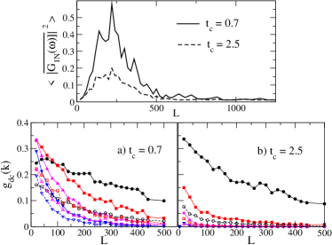
Figure 1: Top panel: Disorder averaged of $\langle\overline{|G^{0}_{1,N}(\omega)|^{2}}\rangle$ in a window of width $\delta\omega=\Phi=0.01$ ($\overline{\{...\}}$ denotes frequency average) as a function of the length $L$ for $t_{c}=0.7$ (solid line) and $t_{c}=2.5$ (dashed line). Lower panel (Color on-line). Contributions to the conductance $g_{dc}(k)$ as a function of $L$ and for the same $\Phi$, for $|k|=1$ (black circles), $|k|=2$ (red squares), $|k|=3$ (magenta up triangles) and $|k|=4$ ( blue down triangles). Solid (open) symbols correspond to $k>0(k<0)$. a) $t_{c}=0.7$ and b) $t_{c}=2.5$, for this coupling the single channel regime is reached for smaller values of $L$. The averages are over 5000 disorder realizations and for ${\cal W}=0.5$.

In Fig.2 we plot, as a function of $L$ and for different couplings $t_{c}$, the disorder averaged conductances $g_{dc}=J_{dc}/\Phi$ (solid line) for the ring coupled to the reservoir and $g_{w}=J_{w}/\Phi$ (dashed line) obtained from Eq.(4) for a 1D wire coupled to both reservoirs with $t_{c}$. For each coupling, we identify a crossover length $L_{c}$ at which the two conductances overlap for $L>L_{c}$. For $t_{c}=1$, $L_{c}\sim l$, being $l$ the localization length obtained for a wire with disorder strength ${\cal W}$ (for the parameters under consideration $l=425$). For other couplings we found that $L_{c}/l$ is a monotonic decreasing function of $t_{c}$. We have verified that for $L>L_{c}$ the regime is single-channel i.e. $g_{dc}\sim g_{dc}(k=1)$ and that it follows the exponential behavior expected for a disorder wire, i.e. $g_{dc}\sim g_{w}\propto\exp{(-L/l)}$. On the other hand, in the “multifloquet” regime for $L<L_{c}$, the two conductances differ dramatically and, in addition, can be $g_{dc}>>1$. In this regime we find a power law behavior $g_{dc}\propto L^{-\alpha_{c}}$, with the exponent $\alpha_{c}$ slightly dependent on the coupling to the reservoir. This is illustrated in the inset of Fig.2 panel d), where we show in solid line the log-log plot of $g_{dc}$ vs $L$ for $t_{c}=2.5$. Our estimates cast $\alpha_{c}=0.3(0.4)$ for $t_{c}=0.7(2.5)$, respectively.

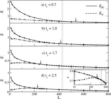
Figure 2: $g_{dc}$ for the disordered ring (solid line) and $g_{w}$ for the $1D$ wire (dashed line) calculated with Eq.(4) with chemical potential difference $\Phi$, as functions of $L$. The different panels correspond are a) $t_{c}=0.7$, b) $t_{c}=1$ c) $t_{c}=1.7$ and c) $t_{c}=2.5$. The localization length $l=425$ for $t_{c}=t_{h}=1$ is shown as a vertical dotted line and the crossover length $L_{c}$ is indicated in each panel by a vertical arrow. Inset: Log-log plot of $g$ vs $L$ for $t_{c}=2.5$. The transition in $g_{dc}$ from the power-law to the exponential decrease with $L$ is at the crossover length $L_{c}\sim 230$. Other details are as in Fig. 1.

So far, we have focused in the mean values of the conductance. In what follows, we present further evidences of the multifloquet to single-channel transition, based on the analysis of the full distribution of the dc conductances. In Fig.3 we plot the distributions $P(g_{dc})$ (solid line histogram) and $P(g_{w})$ (dashed line histogram) for a weak coupling to the reservoir, $t_{c}=0.7$, for which we find $L_{c}\sim 500$. For lengths $L<L_{c}$, that is in the “multifloquet” regime, the distribution $P(g_{dc})$ spreads over a wide range of conductance values, much larger than the maximum allowed for a single channel wire ($g^{max}_{w}=1$). On the other hand, for $L=800>L_{c}$ (panel c)) both histograms correspond to the same Log-normal distribution, characteristic of 1D disordered wires in the localized regime benrev . For completeness, the distributions $P(g_{dc})$ (solid line histogram) and $P(g_{w})$ (dashed line histogram) at a fixed length $L=200$ and as a function of $t_{c}$ are shown in Fig.4. For the strongest coupling considered, $t_{c}=2.5$ (panel d)), the estimate is $L_{c}\sim 230$ (see Fig. 2) and in consistency, $P(g_{dc})$ for $L=200$ closely follows $P(g_{w})$.

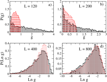
Figure 3: (Color on-line) Conductance distribution $P(g)$ for the disordered ring (black solid line) and wire (red dashed line) for $t_{c}=0.7$ and a) L=120, b) L=200, c) L=400 and d) L=800. Other details are as in Fig. 1.

To conclude, we have identified two regimes in the dc response of a 1D disorder ring threaded by a linear time-dependent magnetic flux and coupled to a reservoir: (i) a “multifloquet” regime that can give rise to high dc currents, significantly larger than those expected in a Landauer setup with an equivalent bias, and (ii) a single channel regime with identical transport behavior as in a Landauer setup, not only in the average conductance but in the complete probability distribution as well. Our results have at least two important outcomes. The first one is that the “multifloquet” regime can support much higher currents than those expected from the naive argument of assuming that only electrons at the Fermi level contribute to the current. This regime should be conceptually equivalent to the “ultra quantum” regime defined in Ref. krav and could be realized, for example, in mesoscopic rings with a low level of disorder and with a very low coupling to the environment. Secondly, it would also take place in rings driven by harmonically time-dependent fields, like for example, a magnetic flux with an harmonic dependence on time, which corresponds to a Hamiltonian with a similar structure as Eq.(1) note . Thus, some conclusions of the present work, in particular the existence of the “multifloquet” regime, should also be valid for Aharanov-Bohm mesoscopic rings with harmonically time-dependent fluxes, in which amplified values of the persistent currents, have been already measured bouchiat . In addition some ab-initio calculations have been recently reported where the mechanism to introduce an electric field in the sample is exactly the one considered in the present work, namely, threading the ring with a time-dependent flux dft . It could be then interesting to check the present predictions by alternative methods.

We acknowledge support from CONICET, Fundación Antorchas PICT 0311609 and PICT 0313829, Argentina, as well as FIS2006-08533-C03-02, the “Ramon y Cajal” program from MCEyC, grant DGA for Groups of Excelence of Spain and the hospitality of Boston University (LA).

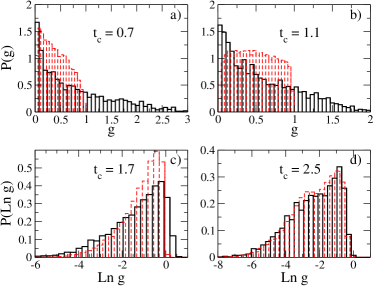
Figure 4: (Color on-line) The same as Fig.3 for $L=200$ and a) $t_{c}=0.7$, b) $t_{c}=1.1$, c) $t_{c}=1.7$ and d) $t_{c}=2.5$.

References

- (1) M. Switkes, et al , Science 283, 1905 (1999).
- (2) M. D. Blumenthal, et al , Nature Physics 3, 343 (2007).
- (3) P.-M. Billangeon, F. Pierre, H. Bouchiat, and R. Deblock Phys. Rev. Lett. 98, 126802 (2007).
- (4) M. Büttiker, Y. Imry and R. Landauer, Phys. Lett. 96A, 367 (1983).
- (5) R. Landauer and M. Büttiker, Phys. Rev. Lett. 54, 2049 (1985).
- (6) R. Landauer, IBM J. Res. Dev. 1, 233 (1957).
- (7) N. Trivedi and D. A. Browne, Phys. Rev. B 38, 9581 (1986).
- (8) B. Reulet and H. Bouchiat, Phys. Rev. B 50, 2259 (1994).
- (9) A. Kamenev and W. Kohn, Phys. Rev. B 63, 155304 (2001).
- (10) C.W.J. Beenakker, Rev. Mod. Phys. 69, 731 (1997) and references therein.
- (11) F. Foieri, et al, Phys. Rev. B 74, 165313 (2006).
- (12) L. Arrachea, Phys. Rev. B 66, 045315 (2002); ibid 70, 155407 (2004)
- (13) L. Arrachea, Phys. Rev. B 72, 125349 (2005); ibid 75, 035319 (2007); L. Arrachea and M. Moskalets, Phys. Rev. B 74, 245322 (2006).
- (14) A. Silva and V. E. Kravtsov, cond-mat/0611083.
- (15) The frequency of the ac flux enters instead of , and additional terms involving higher harmonics of would also contribute to (1).
- (16) R. Deblock, R. Bel, B. Reulet, H. Bouchiat, and D. Mailly, Phys. Rev. Lett. 89, 206803 (2002).
- (17) R. Gebauer and R. Car, Phys. Rev. B 70, 125324 (2004).