Geography of local configurations

Abstract

A $d$-dimensional binary Markov random field on a lattice torus is considered. As the size $n$ of the lattice tends to infinity, potentials $a=a(n)$ and $b=b(n)$ depend on $n$. Precise bounds for the probability for local configurations to occur in a large ball are given. Under some conditions bearing on $a(n)$ and $b(n)$, the distance between copies of different local configurations is estimated according to their weights. Finally, a sufficient condition ensuring that a given local configuration occurs everywhere in the lattice is suggested.

1 Introduction

In the theory of random graphs, inaugurated by Erdős and Rényi ErdosRenyi , the appearance of a given subgraph has been widely studied (see Bollobás Bollobas and Spencer Spencer for general references). In the random graph formed by $n$ vertices, in which the edges are chosen independently with probability $0<p<1$, a subgraph may occur or not according to the value of $p=p(n)$. In addition, under a certain condition on the probability $p(n)$, its number of occurrences in the graph is asymptotically (i.e., as $n\to+\infty$) Poissonian. Replacing the edges with the states of a binary Markov random field, the notion of subgraph corresponds to the notion of what we will call local configuration. Figure 1 shows an example. Many situations can be modeled by binary Markov random fields; a vertex and its state correspond to a pixel and its color (black or white) in image analysis, to an individual and its opinion (yes or no) in sociology or to an atom and its spin (positive or negative) in statistical physics. This last interpretation leads to the well-known Ising model. See KindermannSnell for details.

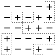
Figure 1: A local configuration $\eta$ with $k(\eta)=|V_{+}(\eta)|=10$ positive vertices and a perimeter $\gamma(\eta)$ equals to $58$, in dimension $d=2$ and on a ball of radius $r=2$ (with $\rho=1$ and relative to the $L_{\infty}$ norm).

Following the theory of random graphs, the appearance of a given local configuration has been investigated in previous works (see Coupier06-2 and CoupierDoukhanYcart ). In this article, this study is extended into three directions. First, the speed at which local configurations occur is specified. Moreover, when the number of copies in the graph of a given local configuration is finite, the states of vertices surrounding one of these copies are described. Finally, a sufficient condition ensuring that a given local configuration is present everywhere in the graph is stated. The results obtained in these three directions are based on the same tools; the Markovian character of the measure, the control of the conditional probability for a local configuration to occur in the graph and the FKG inequality FKG .

Let us consider a lattice graph in dimension $d\geq 1$, with periodic boundary conditions (lattice torus). The vertex set is $V_{n}=\{0,\ldots,n-1\}^{d}$. The integer $n$ will be called the size of the lattice. The edge set, denoted by $E_{n}$, will be specified by defining the set of neighbors $\mathcaligr{V}(x)$ of a given vertex $x$:

$$\mathcaligr{V}(x)=\{y\neq x\in V_{n},\|y-x\|_{q}\leq\rho\},$$ (1)

where the substraction is taken componentwise modulo $n$, $\|\cdot\|_{q}$ stands for the $L_{q}$ norm in $\mathbb{R}^{d}$ ($1\leq q\leq\infty$), and $\rho$ is a fixed integer. For instance, the square lattice is obtained for $q=\rho=1$. Replacing the $L_{1}$ norm with the $L_{\infty}$ norm adds the diagonals. From now on, all operations on vertices will be understood modulo $n$. In particular, each vertex of the lattice has the same number of neighbors; we denote by $\mathcaligr{V}$ this number.

A configuration is a mapping from the vertex set $V_{n}$ to the state space $\{-1,+1\}$. Their set is denoted by $\mathcaligr{X}_{n}=\{-1,+1\}^{V_{n}}$ and called the configuration set. In the following, we shall merely denote by $+$ and $-$ the states $+1$ and $-1$. Let $a$ and $b$ be two reals. The Gibbs measure associated to potentials $a$ and $b$ is the probability measure $\mu_{a,b}$ on $\mathcaligr{X}_{n}=\{-,+\}^{V_{n}}$ defined by: for all $\sigma\in\mathcaligr{X}_{n}$,

$$\mu_{a,b}(\sigma)=\frac{1}{Z_{a,b}}\exp\biggl{(}a\sum_{x\in V_{n}}\sigma(x)+b\sum_{\{x,y\}\in E_{n}}\sigma(x)\sigma(y)\biggr{)},$$ (2)

where the normalizing constant $Z_{a,b}$ is such that $\sum_{\sigma\in\mathcaligr{X}_{n}}\mu_{a,b}(\sigma)=1$. Expectations relative to $\mu_{a,b}$ will be denoted by $\mathbb{E}_{a,b}$. Georgii Georgii and Malyshev and Minlos Malyshev constitute classical references on Gibbs measures.

Throughout this paper, some hypotheses on $a$ and $b$ are made. The model remaining unchanged by swapping positive and negative vertices and replacing $a$ by $-a$, we chose to study only negative values of the potential $a$. Thus, in order to use the FKG inequality, the potential $b$ is supposed nonnegative. Finally, as the size $n$ of the lattice tends to infinity, $a=a(n)$ and $b=b(n)$ are allowed to depend on $n$. The case where $a(n)$ tends to $-\infty$ corresponds to rare positive vertices among a majority of negative ones. So as to simplify formulas, the Gibbs measure $\mu_{a(n),b(n)}$ is still denoted by $\mu_{a,b}$.

In statistical physics, which is the point of view of Coupier06-2 , the probabilistic model previously defined corresponds to the ferromagnetic Ising model. In this context, potentials $a$ and $b$ are, respectively, called the magnetic field and the pair potential.

We are interested in the appearence in the graph $G_{n}$ of families of local configurations. See Section 2 for a precise definition and Figure 1 for an example. Such configurations are called “local” in the sense that the vertex set on which they are defined is fixed and does not depend on $n$. A local configuration $\eta$ is determined by its set of positive vertices $V_{+}(\eta)$ whose cardinality and perimeter are, respectively, denoted by $k(\eta)$ and $\gamma(\eta)$. A natural idea (coming from Coupier06-2 ) consists in regarding both parameters $k(\eta)$ and $\gamma(\eta)$ through the same quantity; the weight of the local configuration $\eta$

$$W_{n}(\eta)=\exp\bigl{(}2a(n)k(\eta)-2b(n)\gamma(\eta)\bigr{)}.$$

This notion plays a central role in our study. Indeed, the weight $W_{n}(\eta)$ represents the probabilistic cost associated to a given occurrence of $\eta$.

Proving some sharp inequalities is generally more difficult than stating only limits. In the case of random graphs, Janson, Łuczak and Ruciński JLR , thus Janson Janson , have obtained exponential bounds for the probability of nonexistence of subgraphs. Some other useful inequalities have been suggested by Boppona and Spencer Boppona . In bond percolation on $\mathbb{Z}^{d}$, it is believed that, in the subcritical phase, the probability for the radius of an open cluster of being larger than $n$ behaves as an exponential term multiplied by a power of $n$; see Grimmett Grimmett , page 85, for precise bounds. But, when the variables of the system are dependent, as the states of a Markov random field, such inequalities become harder to obtain. The Stein–Chen method (see Barbour, Holst and Janson Barbour for a very complete reference or Chen for the original paper of Chen) is a useful way to bound the error of a Poisson approximation and so, in particular, to bound the absolute value of the difference between the probability of a property of the model and its limit. An example of such a property is the appearance of a negative vertex (see Ganesh et al. GHOSU ) or more generally that of any given local configuration Coupier06-1 . These two previous papers concern the case of a divergent potential $|a|$ and a constant potential $b$. Coupling with the loss-network space-time representation due to Fernández, Ferrari and Garcia FFG2 , Ferrari and Picco FerrariPicco have proved an exponential bound for large contours at low temperature (i.e., $b$ large enough) and zero magnetic field (i.e., $a=0$). Finally, under mixing conditions, various exponential approximations with error bounds have been proved; see Abadi and Galves AbadiGalves for an overview and Abadi et al. ACRV for the high temperature case (i.e., $b$ small enough).

Our first goal is to establish precise lower and upper bounds for the probability for certain families of local configurations to occur in the graph for unbounded potentials $a(n)$ and $b(n)$.

Let $x\in V_{n}$ be a vertex, $W\in\,]0,1[$ be a real number and $R$ be an integer. We denote by $\mathcaligr{A}(x,R,W)$ the (interpreted) event “a local configuration whose weight is smaller than $W$ occurs somewhere in the ball of center $x$ and radius $R$.” The study of the probability of this event becomes interesting when the radius $R=R(n)$ and the weight $W=W_{n}$ depend on $n$ and tend, respectively, to infinity and zero. Then, Theorem 4.1 gives precise bounds for the probability of the opposit event ${}^{c}\mathcaligr{A}(x,R(n),W_{n})$. There exist two (explicit) constants $K>K^{\prime}>0$ such that for $n$ large enough,

$$\exp(-KR(n)^{d}W_{n})\leq\mu_{a,b}(^{c}\mathcaligr{A}(x,R(n),W_{n}))\leq\exp(-K^{\prime}R(n)^{d}W_{n}).$$

Another interesting problem consists in describing geographically what happens in the studied model: the size of objects occurring in the model and the distance between them. The size of components in random graphs or the radius of open clusters in percolation are two classical examples (see, respectively, Bollobas and Grimmett ). For the low-temperature plus-phase of the Ising model, Chazottes and Redig ChazottesRedig have studied the appearance of the first two copies of a given pattern in terms of occurrence time and repetition time. The occurrence time $T_{A}$ of a pattern $A$ represents the volume of the smallest set of vertices in which $A$ can be found. As the size of the pattern increases, the distribution of $T_{A}$ is approximated by an exponential law with error bounds. The same is true for the repetition time $R_{A}$. Similar results exist for sufficiently mixing Gibbs random fields (see ACRV ).

In our context, the studied objects are local. Hence, our second goal is to estimate the distance between different copies of local configurations occurring in the graph.

Let $\eta$ be a local configuration. It has been proved in Coupier06-2 that the number of copies of $\eta$ occurring in $G_{n}$ is asymptotically Poissonian provided the product $n^{d}W_{n}(\eta)$ is constant [the precise hypotheses are denoted by (H) and recalled in the beginning of Section 5]. In particular, the number of copies of $\eta$ in the graph is finite with probability tending to $1$. Let $\eta_{x}$ be one of them (that occurring on the ball centered at $x$). We first observe that vertices surrounding $\eta_{x}$ are all negative (Lemma 5.1). Hence, a natural question is the distance from $\eta_{x}$ to the closest positive vertices. Theorem 5.3 answers to this question; it states that the distance from $\eta_{x}$ to the closest local configurations of weight $W_{n}$ is of order $W_{n}^{-1/d}$. Two other results complete the study of the geography of local configurations under the hypothesis (H). Theorem 5.4 claims the distance between the closest local configurations (to $\eta_{x}$) of weight $W_{n}$ is also of order $W_{n}^{-1/d}$. The situation described by Theorems 5.3 and 5.4 is represented in Figure 4. Finally, Theorem 5.3 implies the distance between any two two any copies of $\eta$ should be of order $n$, which is the size of the graph. Proposition 5.5 precises this intuition.

From Coupier06-2 , a condition ensuring that a local configuration $\eta$ occurs in $G_{n}$ is deduced; if the product $n^{d}W_{n}(\eta)$ tends to infinity then, with probability tending to $1$, at least one copy of $\eta$ can be found somewhere in the graph. However, an uncertainty remains about the places in $G_{n}$ where $\eta$ occurs. A richer information would be to know when the local configuration $\eta$ occurs everywhere in $G_{n}$; we will talk about ubiquity of $\eta$. Inequalities stated in the proof of Theorem 4.1 allow us to obtain such an information.

For that purpose, the lattice $V_{n}$ is divided into blocks of $(2R(n)+1)^{d}$ vertices. Thus, a supergraph $\tilde{G}_{n}$ whose set of vertices $\tilde{V}_{n}$ is formed by the centers of these blocks is defined. In order to study the appearance of $\eta$ in each of these blocks, the set of configurations of $\tilde{V}_{n}$ is endowed with an appropriate measure $\tilde{\mu}_{a,b}$ (depending on $\eta$). Proposition 6.2 precises the asymptotic behavior of $\tilde{\mu}_{a,b}$ according to the weight $W_{n}(\eta)$, the radius of the blocks $R(n)$ and the size $n$. In particular, if

$$\lim_{n\to+\infty}R(n)^{d}\ln\biggl{(}\frac{n}{R(n)}\biggr{)}^{-1}W_{n}(\eta)=+\infty,$$

then, with probability tending to $1$, all the blocks contain at least one copy of the local configuration $\eta$.

The paper is organized as follows. The notion of local configuration $\eta$ is defined in Section 2. Its number of positive vertices $k(\eta)$, its perimeter $\gamma(\eta)$ and its weight $W_{n}(\eta)$ are also introduced. Section 3 is devoted to the three main tools of our study. Property 3.1 underlines the Markovian character of the Gibbs measure $\mu_{a,b}$. A control of the conditional probability for a local configuration to occur on a ball uniformly on the neighborhood of that ball is given in Lemma 3.2. Finally, the FKG inequality is discussed at the end of Section 3. Section 4 gives the proof of Theorem 4.1. The geography of local configurations occurring in the graph is described in Section 5. Section 5.1 introduces the problem [the hypothesis (H) and Lemma 5.1]. Theorems 5.3 and 5.4 and Proposition 5.5 are stated in Section 5.2 and proved in Section 5.3. The graph $\tilde{G}_{n}$ and the measure $\tilde{\mu}_{a,b}$ are defined in Section 6. The latter inherits from $\mu_{a,b}$ its Markovian character (Property 6.1). Finally, Proposition 6.2 studies its asymptotic behavior.

2 Local configurations

Let us start with some notation and definitions. Given $\zeta\in\mathcaligr{X}_{n}=\{-,+\}^{V_{n}}$ and $V\subset V_{n}$, we denote by $\zeta_{V}$ the natural projection of $\zeta$ over $\{-,+\}^{V}$. If $U$ and $V$ are two disjoint subsets of $V_{n}$ then $\zeta_{U}\zeta^{\prime}_{V}$ is the configuration on $U\cup V$ which is equal to $\zeta$ on $U$ and $\zeta^{\prime}$ on $V$. Let us denote by $\delta V$ the neighborhood of $V$ [corresponding to (1)]:

$$\delta V=\bigl{\{}y\in V_{n}\setminus V,\exists x\in V,\{x,y\}\in E_{n}\bigr{\}}$$

and by $\overline{V}$ the union of the two disjoint sets $V$ and $\delta V$. Moreover, $|V|$ denotes the cardinality of $V$ and $\mathcaligr{F}(V)$ the $\sigma$-algebra generated by the configurations of $\{-,+\}^{V}$. Finally, if $A\in\mathcaligr{F}(V_{n})$, we denote by ${}^{c}A$ the opposit event.

As usual, the graph distance $\mathrm{dist}$ is defined as the minimal length of a path between two vertices. We shall denote by $B(x,r)$ the ball of center $x$ and radius $r$:

$$B(x,r)=\{y\in V_{n};\operatorname{dist}(x,y)\leq r\}.$$

In the case of balls, $\overline{B(x,r)}=B(x,r+1)$. In order to avoid unpleasant situations, like self-overlapping balls, we will always assume that $n>2\rho r$. If $n$ and $n^{\prime}$ are both larger than $2\rho r$, the balls $B(x,r)$ in $G_{n}$ and $G_{n^{\prime}}$ are isomorphic. Two properties of the balls $B(x,r)$ will be crucial in what follows. The first one is that two balls with the same radius are translates of each other:

$$B(x+y,r)=y+B(x,r).$$

The second one is that for $n>2\rho r$, the cardinality of $B(x,r)$ depends only on $r$ and neither on $x$ nor on $n$: it will be denoted by $\beta_{r}$. Observe that whatever the choices of $q$ and $\rho$ in (1) the ball $B(x,r)$ is included in the sublattice $[x-\rho r,x+\rho r]$, and thus

$$\beta_{r}\leq(2\rho r+1)^{d}.$$

Let $r$ be a positive integer, and consider a fixed ball with radius $r$, say $B(0,r)$. We denote by $\mathcaligr{C}_{r}=\{-,+\}^{B(0,r)}$ the set of configurations on that ball. Elements of $\mathcaligr{C}_{r}$ will be called local configurations with radius $r$, or merely local configurations whenever the radius $r$ will be fixed. Of course, there exists only a finite number of such configurations (precisely $2^{\beta_{r}}$). See Figure 1 for an example. Throughout this paper, the radius $r$ will be constant, that is, it will not depend on the size $n$. Hence, defining local configurations on balls of radius $r$ serves only to ensure that studied objects are “local.” In what follows, $\eta$, $\eta^{\prime}$ will denote local configurations of radius $r$.

A local configuration $\eta\in\mathcaligr{C}_{r}$ is determined by its subset $V_{+}(\eta)\subset B(0,r)$ of positive vertices:

$$V_{+}(\eta)=\{x\in B(0,r),\eta(x)=+\}.$$

The cardinality of this set will be denoted by $k(\eta)$ and its complement in $B(0,r)$, that is, the set of negative vertices of $\eta$, by $V_{-}(\eta)$. Moreover, the geometry (in the sense of the graph structure) of the set $V_{+}(\eta)$ needs to be described. Let us define the perimeter $\gamma(\eta)$ of the local configuration $\eta$ by the formula

$$\gamma(\eta)=\mathcaligr{V}|V_{+}(\eta)|-2\bigl{|}\bigl{\{}\{x,y\}\in V_{+}(\eta)\times V_{+}(\eta),\{x,y\}\in E_{n}\bigr{\}}\bigr{|},$$

where $\mathcaligr{V}$ is the number of neighbors of a vertex. In other words, $\gamma(\eta)$ counts the pairs of neighboring vertices $x$ and $y$ of $B(0,r)$ having opposite spins (under $\eta$) and those such that $x\in B(0,r)$, $y\in\delta B(0,r)$ and $\eta(x)=+$.

We denote by $W_{n}(\eta)$ and call the weight of the local configuration $\eta$ the following quantity:

$$W_{n}(\eta)=\exp\bigl{(}2a(n)k(\eta)-2b(n)\gamma(\eta)\bigr{)}.$$

Since $a(n)<0$ and $b(n)\geq 0$, the weight $W_{n}(\eta)$ satisfies $0<W_{n}(\eta)\leq 1$. That of the local configuration having only negative vertices, denoted by $\eta_{-}$ and called the negative local configuration, is equal to $1$. If $\eta\not=\eta_{-}$ then $k(\eta)\geq 1$ and $\gamma(\eta)\geq\mathcaligr{V}$. It follows that

$$W_{n}(\eta)\leq\exp\bigl{(}2a(n)-2b(n)\mathcaligr{V}\bigr{)}.$$

Actually, the weight $W_{n}(\eta)$ represents the probabilistic cost associated to the presence of $\eta$ on a given ball. This idea will be clarified in the next section (Lemma 3.2).

Remark the notation $k(\cdot)$, $\gamma(\cdot)$ and $W_{n}(\cdot)$ can be naturally extended to any configuration $\zeta\in\{-,+\}^{V}$, $V\subset V_{n}$.

Let $\eta\in\mathcaligr{C}_{r}$. For each vertex $x\in V_{n}$, denote by $\eta_{x}$ the translation of $\eta$ onto the ball $B(x,r)$ (up to periodic boundary conditions):

$$\forall y\in V_{n}\qquad\operatorname{dist}(0,y)\leq r\quad\Longrightarrow\quad\eta_{x}(x+y)=\eta(y).$$

In particular, $V_{+}(\eta_{x})=x+V_{+}(\eta)$. So, $\eta$ and $\eta_{x}$ have the same number of positive vertices and the same perimeter. So do their weights. Let us denote by $I_{x}^{\eta}$ the indicator function defined on $\mathcaligr{X}_{n}$ as follows: $I_{x}^{\eta}(\sigma)$ is $1$ if the restriction of the configuration $\sigma\in\mathcaligr{X}_{n}$ to the ball $B(x,r)$ is $\eta_{x}$ and $0$ otherwise.

Let $V$ and $V^{\prime}$ be two disjoint subsets of vertices. The following relations

$$k(\zeta\zeta^{\prime})=k(\zeta)+k(\zeta^{\prime})\quad\mbox{and}\quad\gamma(\zeta\zeta^{\prime})\leq\gamma(\zeta)+\gamma(\zeta^{\prime})$$

are true whatever the configurations $\zeta\in\{-,+\}^{V}$ and $\zeta^{\prime}\in\{-,+\}^{V^{\prime}}$. As an immediate consequence, the weight $W_{n}(\zeta\zeta^{\prime})$ is larger than the product $W_{n}(\zeta)W_{n}(\zeta^{\prime})$. The connection between $\zeta\in\{-,+\}^{V}$ and $\zeta^{\prime}\in\{-,+\}^{V^{\prime}}$, denoted by $\operatorname{conn}(\zeta,\zeta^{\prime})$, is defined by

$$\operatorname{conn}(\zeta,\zeta^{\prime})=\bigl{|}\bigl{\{}\{y,z\}\in E_{n},y\in V,z\in V^{\prime}\mbox{ and }\zeta(y)=\zeta^{\prime}(z)=+\bigr{\}}\bigr{|}.$$

This quantity allows us to link the perimeters of the configurations $\zeta\zeta^{\prime}$, $\zeta$ and $\zeta^{\prime}$ together:

$$\gamma(\zeta\zeta^{\prime})+2\operatorname{conn}(\zeta,\zeta^{\prime})=\gamma(\zeta)+\gamma(\zeta^{\prime})$$

and therefore their weights:

$$W_{n}(\zeta\zeta^{\prime})\exp(-4b(n)\operatorname{conn}(\zeta,\zeta^{\prime}))=W_{n}(\zeta)W_{n}(\zeta^{\prime}).$$ (3)

In particular, if the connection $\operatorname{conn}(\zeta,\zeta^{\prime})$ is null then the weight $W_{n}(\zeta\zeta^{\prime})$ is equal to the product $W_{n}(\zeta)W_{n}(\zeta^{\prime})$. This is the case when $\overline{V}\cap V^{\prime}=\varnothing$.

3 The three main tools

This section is devoted to the main tools on which are based all the results of this paper: the Markovian character of the Gibbs measure $\mu_{a,b}$, a control of the probability for $\eta\in\mathcaligr{C}_{r}$ to occur on a given ball and the FKG inequality. Except the first part of Lemma 3.2, the results of this section are already known.

Two subsets of vertices $U$ and $V$ of $V_{n}$ are said $\mathcaligr{V}$-disjoint if none of the vertices of $U$ belong to the neighborhood of one of the vertices of $V$. In other words, $U$ and $V$ are $\mathcaligr{V}$-disjoint if and only if $U\cap\overline{V}=\varnothing$ (or equivalently $\overline{U}\cap V=\varnothing$). For example, two balls $B(x,r)$ and $B(x^{\prime},r)$ are $\mathcaligr{V}$-disjoint if and only if the distance between their centers $x$ and $x^{\prime}$ is larger than $2r+1$, that is, $\operatorname{dist}(x,x^{\prime})>2r+1$.

The following result is a classical property of Gibbs measures (see Georgii , page 157); it describes the Markovian character of $\mu_{a,b}$. The second part of Property 3.1 means that, given two $\mathcaligr{V}$-disjoint sets $U$ and $V$, the $\sigma$-algebras $\mathcaligr{F}(U)$ and $\mathcaligr{F}(V)$ are conditionally independent knowing the configuration on $\delta U\cup\delta V$.

For any sets of vertices $V,V^{\prime}$ and for any event $A\in\mathcaligr{F}(V)$, the function $\mu_{a,b}(A|\mathcaligr{F}(V^{\prime}))$ denotes the $\mathcaligr{F}(V^{\prime})$-measurable random variable defined as follows; for $\sigma\in\{-,+\}^{V^{\prime}}$, $\mu_{a,b}(A|\mathcaligr{F}(V^{\prime}))(\sigma)$ is the conditional probability $\mu_{a,b}(A|\sigma)$.

Property 3.1

Let $V,V^{\prime}\subset V_{n}$ be two sets of vertices such that $V\cap V^{\prime}=\varnothing$ and $\delta V\subset V^{\prime}$. Then, for all $A\in\mathcaligr{F}(V)$,

$$\mu_{a,b}(A|\mathcaligr{F}(V^{\prime}))=\mu_{a,b}(A|\mathcaligr{F}(\delta V)).$$ (4)

Let $U,V,V^{\prime}\subset V_{n}$ be three sets of vertices such that $U$ and $V$ are $\mathcaligr{V}$-disjoint, $(U\cup V)\cap V^{\prime}=\varnothing$ and $\delta U\cup\delta V\subset V^{\prime}$. Then, for all $A\in\mathcaligr{F}(U)$ and $B\in\mathcaligr{F}(V)$,

$$\mu_{a,b}\bigl{(}A\cap B|\mathcaligr{F}(V^{\prime})\bigr{)}=\mu_{a,b}(A|\mathcaligr{F}(V^{\prime}))\mu_{a,b}(B|\mathcaligr{F}(V^{\prime})).$$ (5)

Let us note that (4) is a consequence of the identity

$$\forall\sigma\in\{-,+\}^{\delta V},\forall\sigma^{\prime}\in\{-,+\}^{V^{\prime}\setminus\delta V}\qquad\mu_{a,b}(A|\sigma\sigma^{\prime})=\mu_{a,b}(A|\sigma),$$

which itself relies on the exponential form of the Gibbs measure $\mu_{a,b}$ [see (2)]. The proof of a similar identity is available in Malyshev , page 7.

Besides, the second part of Property 3.1 can be immediatly extended to any finite family of sets of vertices which are two by two $\mathcaligr{V}$-disjoint. This remark will be used often in the following.

Let $\eta$ be a local configuration. Thanks to the translation invariance of the graph $G_{n}$, the indicator functions $I_{x}^{\eta}$, $x\in V_{n}$, have the same distribution. So, let us pick a vertex $x$. For any configuration $\sigma\in\{-,+\}^{\delta B(x,r)}$, the quantity $\mu_{a,b}(I_{x}^{\eta}=1|\sigma)$ represents the probability for $\eta$ (or $\eta_{x}$) to occur on the ball $B(x,r)$ knowing what happens on its neighborhood. A precise study of this conditional probability has been done in Coupier06-2 , Section 2. From there, a control is deduced:

Lemma 3.2

Let $\eta$ be a local configuration with radius $r$, and $x$ be a vertex.

On the one hand, if $a(n)+\mathcaligr{V}b(n)\leq 0$ then there exists a constant $c_{r}>0$ such that, for all configuration $\sigma\in\{-,+\}^{\delta B(x,r)}$,

$$\mu_{a,b}(I_{x}^{\eta}=1|\sigma)\geq c_{r}W_{n}(\eta).$$ (6)

In particular, $\mu_{a,b}(I_{x}^{\eta}=1)$ satisfies the same lower bound. On the other hand, if $a(n)+2\mathcaligr{V}b(n)\leq 0$ then there exists a constant $C_{r}>0$ such that

$$\mu_{a,b}(I_{x}^{\eta}=1)\leq C_{r}W_{n}(\eta).$$ (7)

The constants $C_{r}$ and $c_{r}$ depend on the radius $r$ and on parameters $q$, $\rho$ and $d$ but not on the local configuration $\eta$ nor on $n$. Proof of Lemma 3.2 Let $\eta$ be a local configuration with radius $r$, $x$ be a vertex and $\sigma$ be an element of $\{-,+\}^{\delta B(x,r)}$. Lemma 2.2 of Coupier06-2 allows us to write the conditional probability $\mu_{a,b}(I_{x}^{\eta}=1|\sigma)$ as a function of weights of some configurations:

$$\mu_{a,b}(I_{x}^{\eta}=1|\sigma) = \frac{W_{n}(\eta_{x}\sigma)}{\sum_{\eta^{\prime}\in\mathcaligr{C}_{r}}W_{n}(\eta^{\prime}_{x}\sigma)}$$

$$\geq W_{n}(\eta)\biggl{(}\sum_{\eta^{\prime}\in\mathcaligr{C}_{r}}\frac{W_{n}(\eta^{\prime}_{x}\sigma)}{W_{n}(\sigma)}\biggr{)}^{-1},$$

using the inequality $W_{n}(\eta_{x}\sigma)\geq W_{n}(\eta)W_{n}(\sigma)$. Let $\eta^{\prime}$ be a local configuration. Its perimeter $\gamma(\eta^{\prime})$ can be bounded as follows:

$$\mathcaligr{V}k(\eta^{\prime})\geq\gamma(\eta^{\prime})\geq\operatorname{conn}(\eta^{\prime}_{x},\sigma).$$

Hence, $\gamma(\eta^{\prime})+\mathcaligr{V}k(\eta^{\prime})$ is larger than $2\operatorname{conn}(\eta^{\prime}_{x},\sigma)$ and the difference $\gamma(\eta^{\prime}_{x}\sigma)-\gamma(\sigma)$ satisfies

$$\gamma(\eta^{\prime}_{x}\sigma)-\gamma(\sigma) = \gamma(\eta^{\prime})-2\operatorname{conn}(\eta^{\prime}_{x},\sigma)$$

$$\geq -\mathcaligr{V}k(\eta^{\prime}).$$

We deduce from this last inequality that

$$\frac{W_{n}(\eta^{\prime}_{x}\sigma)}{W_{n}(\sigma)} = \exp\bigl{(}2a(n)k(\eta^{\prime})-2b(n)\bigl{(}\gamma(\eta^{\prime}_{x}\sigma)-\gamma(\sigma)\bigr{)}\bigr{)}$$

$$\leq \exp\bigl{(}\bigl{(}2a(n)+2\mathcaligr{V}b(n)\bigr{)}k(\eta^{\prime})\bigr{)}.$$

Now, the hypothesis $a(n)+\mathcaligr{V}b(n)\leq 0$ implies the ratio $W_{n}(\eta^{\prime}_{x}\sigma)$ divided by $W_{n}(\sigma)$ is smaller than $1$. Thanks to (3), the conditional probability $\mu_{a,b}(I_{x}^{\eta}=1|\sigma)$ is larger than $|\mathcaligr{C}_{r}|^{-1}W_{n}(\eta)$; $c_{r}=|\mathcaligr{C}_{r}|^{-1}=2^{-\beta_{r}}$ is suitable.

Since the lower bound of (6) is uniform on the configuration $\sigma\in\{-,+\}^{\delta B(x,r)}$, the same inequality holds for

$$\mu_{a,b}(I_{x}^{\eta}=1)=\mathbb{E}_{a,b}\bigl{[}\mu_{a,b}\bigl{(}I_{x}^{\eta}=1|\mathcaligr{F}(\delta B(x,r))\bigr{)}\bigr{]}.$$

Finally, (7) has been proved in Proposition 3.2 of Coupier06-2 with $C_{r}=2^{\mathcaligr{V}\beta_{r}}$.

The lower bound given by (6) has the advantage of being uniform on the configuration $\sigma\in\{-,+\}^{\delta B(x,r)}$. In addition, there is no uniform upper bound for the conditional probability $\mu_{a,b}(I_{x}^{\eta}=1|\sigma)$. In order to make up for this gap, we will have recourse to the FKG inequality.

There is a natural partial ordering on the configuration set $\mathcaligr{X}_{n}=\{-,+\}^{V_{n}}$ defined by $\sigma\leq\sigma^{\prime}$ if $\sigma(x)\leq\sigma^{\prime}(x)$ for all vertices $x\in V_{n}$. A real function defined on $\mathcaligr{X}_{n}$ is increasing if $f(\sigma)\leq f(\sigma^{\prime})$ whenever $\sigma\leq\sigma^{\prime}$. An event $A\in\mathcaligr{F}(V_{n})$ is also said increasing whenever its indicator function $f=\mathbh{1}_{A}$ is increasing. Conversely, a decreasing event is an event whose complementary set [in $\mathcaligr{F}(V_{n})$] is increasing.

Let us focus on an example of increasing event which will be central in our study. For $0\leq W\leq 1$, we denote by $\mathcaligr{C}_{r}(W)$ the set of local configurations with radius $r$ whose weight is smaller than $W$:

$$\mathcaligr{C}_{r}(W)=\{\eta\in\mathcaligr{C}_{r},W_{n}(\eta)\leq W\}.$$

Thus, let us consider two local configurations $\eta$, $\eta^{\prime}$ such that the set of positive vertices of $\eta^{\prime}$ contains that of $\eta$. The perimeter $\gamma(\eta^{\prime})$ is not necessary larger than $\gamma(\eta)$: roughly, $V_{+}(\eta)$ may have holes. However, the inequality

$$\gamma(\eta^{\prime})\geq\gamma(\eta)-\bigl{(}k(\eta^{\prime})-k(\eta)\bigr{)}\mathcaligr{V}$$

holds. Hence, the ratio

$$\frac{W_{n}(\eta^{\prime})}{W_{n}(\eta)} = \exp\bigl{(}2a(n)\bigl{(}k(\eta^{\prime})-k(\eta)\bigr{)}-2b(n)\bigl{(}\gamma(\eta^{\prime})-\gamma(\eta)\bigr{)}\bigr{)}$$

$$\leq \exp\bigl{(}\bigl{(}2a(n)+2\mathcaligr{V}b(n)\bigr{)}\bigl{(}k(\eta^{\prime})-k(\eta)\bigr{)}\bigr{)}$$

is smaller than $1$ whenever $a(n)+\mathcaligr{V}b(n)$ is negative. As a consequence, under this hypothesis, the set $\mathcaligr{C}_{r}(W)$ allows us to build some increasing events; for instance,

$$\bigcup_{\eta\in\mathcaligr{C}_{r}(W)}\{I_{x}^{\eta}=1\}.$$

For a positive value of the pair potential $b$, the Gibbs measure $\mu_{a,b}$ defined by (2) satisfies the FKG inequality, that is,

$$\mu_{a,b}(A\cap A^{\prime})\geq\mu_{a,b}(A)\mu_{a,b}(A^{\prime})$$ (9)

for all increasing events $A$ and $A^{\prime}$. See, for instance, Section 3 of FKG . In statistical physics, the hypothesis $b\geq 0$ corresponds to ferromagnetic interaction. Note that inequality (9) can be easily extended to decreasing events (see Grimmett ). Moreover, the union and the intersection of increasing events are still increasing. The same is true for decreasing events. Hence, the FKG inequality applies to any family made up of a finite number of decreasing events $A_{1},\ldots,A_{m}$:

$$\mu_{a,b}(A_{1}\cap\cdots\cap A_{m})\geq\mu_{a,b}(A_{1})\cdots\mu_{a,b}(A_{m}).$$

4 Exponential bounds for the probability of nonexistence

Let $x\in V_{n}$ be a vertex, $R\geq r\geq 1$ be two integers and $W$ be a positive real. Let us denote by $\mathcaligr{A}(x,R,W)$ the following event:

$$\exists y\in B(x,R-r),\exists\eta\in\mathcaligr{C}_{r}(W)\qquad I_{y}^{\eta}=1.$$

The event $\mathcaligr{A}(x,R,W)$ means at least one copy of a local configuration (with radius $r$) whose weight is smaller than $W$ can be found somewhere in the large ball $B(x,R)$. Theorem 4.1 gives exponential bounds for the probability of the opposite event ${}^{c}\mathcaligr{A}(x,R(n),W_{n})$.

Theorem 4.1

Assume that the magnetic field $a(n)$ is negative, the pair potential $b(n)$ is nonnegative and they satisfy $a(n)+2\mathcaligr{V}b(n)\leq 0$. Let $(W_{n})_{n\in\mathbb{N}}$ be a sequence of positive reals satisfying the following property: there exist an integer $N$ and $0<\epsilon<1$ such that

$$\forall n\geq N\qquad\min_{\eta\in\mathcaligr{C}_{r}}W_{n}(\eta)\leq W_{n}\leq\epsilon c_{r}C_{r}^{-1}.$$

Let $K=(2\rho)^{d}(1-\epsilon)^{-1}c_{r}^{-1}C_{r}$ and $K^{\prime}=\tau c_{r}$. Then, for all $n\geq N$ and for all vertex $x$,

$$\quad\exp(-KR(n)^{d}W_{n})\leq\mu_{a,b}(^{c}\mathcaligr{A}(x,R(n),W_{n}))\leq\exp(-K^{\prime}R(n)^{d}W_{n}).$$ (10)

Remark the constants $K$ and $K^{\prime}$ only depend on $r$, $\epsilon$ and parameters $q$, $\rho$ and $d$ (the constant $\tau$ will be introduced in the proof).

The fact that, for $n$ large enough, $W_{n}$ is assumed larger than the smallest weight $W_{n}(\eta)$, $\eta\in\mathcaligr{C}_{r}$, only serves to ensure that the set $\mathcaligr{C}_{r}(W_{n})$ [and the event $\mathcaligr{A}(x,R(n),W_{n})$ too] is nonempty. Moreover, let us note hypothesis $W_{n}\leq\epsilon c_{r}C_{r}^{-1}$ is only used in the proof of the lower bound of (10).

The inequalities of (10) give a limit for the probability of $\mathcaligr{A}(x,R(n),W_{n})$:

$$\mbox{if }\lim_{n\to+\infty}R(n)^{d}W_{n}=0\qquad\mbox{then }\lim_{n\to+\infty}\mu_{a,b}(\mathcaligr{A}(x,R(n),W_{n}))=0;$$

$$\mbox{if }\lim_{n\to+\infty}R(n)^{d}W_{n}=+\infty\qquad\mbox{then }\lim_{n\to+\infty}\mu_{a,b}(\mathcaligr{A}(x,R(n),W_{n}))=1.$$

Roughly speaking, if the radius $R(n)$ is small compared to $W_{n}^{-1/d}$, then asymptotically, with probability tending to $1$, there is no local configuration whose weight is smaller than $W_{n}$. Conversely, if $R(n)$ is large compared to $W_{n}^{-1/d}$ then at least one copy of an element of $\mathcaligr{C}_{r}(W_{n})$ can be found somewhere in $B(x,R(n))$, with probability tending to $1$.

Finally, Theorem 4.1 implies the quantity

$$\frac{1}{R(n)^{d}W_{n}}\ln(\mu_{a,b}(^{c}\mathcaligr{A}(x,R(n),W_{n})))$$ (11)

belongs to the interval $[-K,-K^{\prime}]$. A natural question is to wonder whether (11) admits a limit as $n$ goes to infinity. It seems to be difficult to answer to this question in general. However, in the following particular case, the answer is positive and the corresponding limit is known; see Coupierthese or Coupier06-1 for more details. Assume the weight $W_{n}=W_{n}(\eta)$ is the one of a local configuration $\eta$, the pair potential $b(n)=b$ is a positive real number and the magnetic field $a(n)$ tends to $-\infty$. Under these conditions, the limit of the probability for a given local configuration to occur on the ball $B(x,R(n))$ essentially depends on its number of positive vertices. Moreover, assume the radius $R(n)$ is such that the product $R(n)^{d}W_{n}=R(n)^{d}W_{n}(\eta)$ is constant. Then, the quantity (11) converges, as $n\to+\infty$, to

$$-\mathop{\mathop{\sum}_{\eta^{\prime}\in\mathcaligr{C}_{r}}}_{k(\eta^{\prime})=k(\eta)}\exp\bigl{(}-2b\bigl{(}\gamma(\eta^{\prime})-\gamma(\eta)\bigr{)}\bigr{)}.$$

This section ends with the proof of Theorem 4.1. Proof of Theorem 4.1 Throughout this proof, potentials $a(n)$ and $b(n)$, and the sequence $(W_{n})_{n\in\mathbb{N}}$ satisfy the hypotheses of Theorem 4.1.

The two following remarks will lighten notation and formulas of the proof. Thanks to the invariance translation of the graph $G_{n}$ it suffices to prove Theorem 4.1 for $x=0$. Hence, we merely denote by $\mathcaligr{A}(R(n),W_{n})$ the event $\mathcaligr{A}(0,R(n),W_{n})$. Furthermore, $\mathcaligr{A}(R(n),W_{n})$ and $\mathcaligr{A}(R(n),W_{n}^{\prime})$ are equal for

$$W_{n}^{\prime}=\max_{\eta\in\mathcaligr{C}_{r}(W_{n})}W_{n}(\eta).$$

As a consequence and without loss of generality, we can assume that, for each $n$, the weight $W_{n}$ belongs to $\{W_{n}(\eta),\eta\in\mathcaligr{C}_{r}\}$.

The proof of the lower bound of (10) requires the ferromagnetic character of the probabilistic model, that is, the positivity of the pair potential $b(n)$. Since $a(n)+\mathcaligr{V}b(n)$ is negative, the event

$$\bigcap_{\eta\in\mathcaligr{C}_{r}(W_{n})}\{I_{y}^{\eta}=0\}$$

is decreasing, whatever the vertex $y$. So the FKG inequality implies

$$\mu_{a,b}(^{c}\mathcaligr{A}(R(n),W_{n}))\geq\prod_{y\in B(0,R(n)-r)}\mu_{a,b}\biggl{(}\bigcap_{\eta\in\mathcaligr{C}_{r}(W_{n})}\{I_{y}^{\eta}=0\}\biggr{)}.$$ (12)

Now, it suffices to control each term of the above product. This is the role of Lemma 3.2. Let us pick $y\in B(0,R(n)-r)$. We get

$$\mu_{a,b}\biggl{(}\bigcap_{\eta\in\mathcaligr{C}_{r}(W_{n})}\{I_{y}^{\eta}=0\}\biggr{)} = 1-\sum_{\eta\in\mathcaligr{C}_{r}(W_{n})}\mu_{a,b}(I_{y}^{\eta}=1)$$

$$\geq 1-\sum_{\eta\in\mathcaligr{C}_{r}(W_{n})}C_{r}W_{n}(\eta)$$

$$\geq 1-c_{r}^{-1}C_{r}W_{n},$$

since $|\mathcaligr{C}_{r}(W_{n})|\leq|\mathcaligr{C}_{r}|=c_{r}^{-1}$. Let $N$ be the integer introduced in the statement of Theorem 4.1 and let $n\geq N$. Therefore, from (12) and the inequality $\ln(1-X)\geq-(1-\epsilon)^{-1}X$ valid for $0\leq X\leq\epsilon$, it follows that

$$\mu_{a,b}(^{c}\mathcaligr{A}(R(n),W_{n})) \geq (1-c_{r}^{-1}C_{r}W_{n})^{(2\rho R(n))^{d}}$$

$$\geq \exp\bigl{(}-(2\rho)^{d}(1-\epsilon)^{-1}c_{r}^{-1}C_{r}R(n)^{d}W_{n}\bigr{)}.$$

So, the lower bound of (10) is proved with $K=(2\rho)^{d}(1-\epsilon)^{-1}c_{r}^{-1}C_{r}$.

In order to prove the upper bound of (10), let us denote by $T_{n}$ the subset of $V_{n}$ defined by

$$T_{n}=\biggl{\{}i\bigl{(}\rho(2r+1)+1\bigr{)},|i|=0,\ldots,\biggl{\lfloor}\frac{\rho R(n)}{\rho(2r+1)+1}\biggr{\rfloor}-1\biggr{\}}^{d}\cap B\bigl{(}0,R(n)-r\bigr{)}.$$

Its cardinality, denoted by $\tau_{n}$, satisfies $\tau_{n}\geq\tau R(n)^{d}$, for a positive constant $\tau>0$ not depending on the size $n$. Let $\mathcaligr{T}_{n}$ be the union of the balls with radius $r$ centered at the elements of $T_{n}$ (see Figure 2)

$$\mathcaligr{T}_{n}=\bigcup_{y\in T_{n}}B(y,r)$$

and denote by $\Gamma_{n}$ the event which means an element of $\mathcaligr{C}_{r}(W_{n})$ occurs on a ball $B(y,r)$, $y\in T_{n}$:

$$\Gamma_{n}=\bigcup_{y\in T_{n}}\bigcup_{\eta\in\mathcaligr{C}_{r}(W_{n})}\{I_{y}^{\eta}=1\}.$$

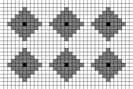
Figure 2: The colored vertices represent the set $\mathcaligr{T}_{n}$ in dimension $d=2$, with $r=2$, $\rho=2$ and relative to the $L_{1}$ norm. The black vertices are elements of $T_{n}$.

Since the balls $B(y,r)$, $y\in T_{n}$, are included in $B(0,R(n))$, the event $\Gamma_{n}$ implies $\mathcaligr{A}(R(n),W_{n})$. So, the upper bound of (10) follows from the next statement. Let $K^{\prime}=\tau c_{r}$. Then, for all $n$,

$$\mu_{a,b}(^{c}\Gamma_{n})\leq\exp(-K^{\prime}R(n)^{d}W_{n}).$$ (13)

Let us prove this inequality. Remark that any two balls $B(y,r)$ and $B(y^{\prime},r)$ where $y$ and $y^{\prime}$ are distinct vertices of $T_{n}$ are $\mathcaligr{V}$-disjoint. Indeed, by construction of the set $T_{n}$, $\operatorname{dist}(y,y^{\prime})>2r+1$. Hence, Property 3.1 produces the following identities:

$$\mu_{a,b}(^{c}\Gamma_{n}) = \mathbb{E}_{a,b}[\mu_{a,b}(^{c}\Gamma_{n}|\mathcaligr{F}(\delta\mathcaligr{T}_{n}))]$$

$$= \mathbb{E}_{a,b}\biggl{[}\mu_{a,b}\biggl{(}\bigcap_{y\in T_{n}}\bigcap_{\eta\in\mathcaligr{C}_{r}(W_{n})}I_{y}^{\eta}=0\Big{|}\mathcaligr{F}(\delta\mathcaligr{T}_{n})\biggr{)}\biggr{]}$$

$$= \mathbb{E}_{a,b}\biggl{[}\prod_{y\in T_{n}}\mu_{a,b}\biggl{(}\bigcap_{\eta\in\mathcaligr{C}_{r}(W_{n})}I_{y}^{\eta}=0\Big{|}\mathcaligr{F}(\delta\mathcaligr{T}_{n})\biggr{)}\biggr{]}$$

$$= \mathbb{E}_{a,b}\biggl{[}\prod_{y\in T_{n}}\mu_{a,b}\biggl{(}\bigcap_{\eta\in\mathcaligr{C}_{r}(W_{n})}I_{y}^{\eta}=0\Big{|}\mathcaligr{F}(\delta B(y,r))\biggr{)}\biggr{]}.$$

Now, let $y\in T_{n}$ be a vertex and $\sigma\in\{-,+\}^{\delta B(y,r)}$ be a configuration. We can write

$$\mu_{a,b}\biggl{(}\bigcap_{\eta\in\mathcaligr{C}_{r}(W_{n})}I_{y}^{\eta}=0\Big{|}\sigma\biggr{)} = 1-\mu_{a,b}\biggl{(}\bigcup_{\eta\in\mathcaligr{C}_{r}(W_{n})}I_{y}^{\eta}=1\Big{|}\sigma\biggr{)}$$

$$\leq 1-\mu_{a,b}(I_{y}^{\eta}=1|\sigma),$$

where $\eta$ is an element of $\mathcaligr{C}_{r}(W_{n})$ satisfying $W_{n}(\eta)=W_{n}$. Lemma 3.2 gives a bound for (4) which does not depend on the configuration $\sigma\in\{-,+\}^{\delta B(y,r)}$ nor on the vertex $y$. Hence, it follows from (4)

$$\mu_{a,b}(^{c}\Gamma_{n})\leq(1-c_{r}W_{n})^{\tau_{n}}$$

(recall that $1-c_{r}W_{n}$ is positive). Finally, using $\tau_{n}\geq\tau R(n)^{d}$ and the classical inequality $\ln(1+X)\leq X$ valid for $X>-1$, a bound for the probability of $X_{n}$ to be null is obtained:

$$\mu_{a,b}(^{c}\Gamma_{n})\leq\exp(-\tau R(n)^{d}c_{r}W_{n}).$$

Inequality (13) is proved with $K^{\prime}=\tau c_{r}$.

5 Distance between local configurations

5.1 Motivation

Throughout Section 5, $\eta$ represents a local configuration with radius $r$ having at least one positive vertex, that is, different from the negative local configuration $\eta_{-}$. The goal of this section is to describe the model under the hypothesis (H), bearing on the potentials $a(n)$ and $b(n)$, and defined by

$$\cases{n^{d}W_{n}(\eta)=\lambda,&\quad for $\lambda>0$,\cr a(n)+2\mathcaligr{V}b(n)\leq 0,\cr a(n)+\mathcaligr{V}b(n)\to-\infty,&\quad as $n\to+\infty$.}$$ (H)

Let us start by giving the reason for (H). Let $X_{n}(\eta)$ be the random variable which counts the number of copies of $\eta$ in the whole graph $G_{n}$:

$$X_{n}(\eta)=\sum_{x\in V_{n}}I_{x}^{\eta}.$$

In Coupier06-2 , various results have been stated about the variable $X_{n}(\eta)$. If the product $n^{d}W_{n}(\eta)$ tends to $0$ (resp., $+\infty$) then the probability $\mu_{a,b}(X_{n}(\eta)>0)$ tends to $0$ (resp., $1$). In other words, if $W_{n}(\eta)$ is small compared to $n^{-d}$, then asymptotically, there is no occurrence of $\eta$ in $G_{n}$. If $W_{n}(\eta)$ is large compared to $n^{-d}$, then at least one occurrence of $\eta$ can be found in the graph, with probability tending to $1$. Moreover, provided the hypothesis (H) is satisfied [in particular $W_{n}(\eta)$ is of order $n^{-d}$], the distribution of $X_{n}(\eta)$ converges weakly to the Poisson distribution with parameter $\lambda$.

In particular, the number of copies of $\eta$ occurring in the graph is finite. Let $\eta_{x}$ be one of them (that occurring on the ball centered at $x$). Lemma 5.1 says vertices around $\eta_{x}$ are negative with probability tending to $1$. For that purpose, let us introduce the ring $\mathcaligr{R}(x,r,R)$ defined as the following set of vertices:

$$\mathcaligr{R}(x,r,R)=\{y\in V_{n},r<\operatorname{dist}(x,y)\leq R\}.$$

Lemma 5.1

Let $\eta$ be a local configuration with radius $r$ and let $x\in V_{n}$. Let us denote by $\mathcaligr{A}_{r}(x,R,+)$ the (interpreted) event “there exists at least one positive vertex in $\mathcaligr{R}(x,r,R)$.”

If the potentials satisfy $a(n)+2\mathcaligr{V}b(n)\leq 0$ and $a(n)\to-\infty$. Then,

$$\lim_{n\to+\infty}\mu_{a,b}\bigl{(}\mathcaligr{A}_{r}(x,R,+)|I_{x}^{\eta}=1\bigr{)}=0.$$

Let us introduce the set $\mathcaligr{C}_{R}(\eta,+)$ formed from local configurations with radius $R$ whose restriction to the ball $B(0,r)$ is equal to $\eta$ and having at least one positive vertex in the ring $\mathcaligr{R}(0,r,R)$:

$$\mathcaligr{C}_{R}(\eta,+)=\{\zeta\in\mathcaligr{C}_{R},\forall y\in B(0,r),\zeta(y)=\eta(y)\mbox{ and }k(\zeta)>k(\eta)\}.$$

The intersection of the events $\mathcaligr{A}_{r}(x,R,+)$ and $I_{x}^{\eta}=1$ forces the ball $B(x,R)$ to contain at least $k(\eta)+1$ positive vertices. Precisely,

$$\mathcaligr{A}_{r}(x,R,+)\cap\{I_{x}^{\eta}=1\}=\bigcup_{\zeta\in\mathcaligr{C}_{R}(\eta,+)}\{I_{x}^{\zeta}=1\}.$$

Then, Lemma 3.2 allows us to bound the probability of that intersection:

$$\mu_{a,b}\bigl{(}\mathcaligr{A}_{r}(x,R,+)\cap\{I_{x}^{\eta}=1\}\bigr{)} \leq \sum_{\zeta\in\mathcaligr{C}_{R}(\eta,+)}\mu_{a,b}(I_{x}^{\zeta}=1)$$

$$\leq C_{R}\sum_{\zeta\in\mathcaligr{C}_{R}(\eta,+)}W_{n}(\zeta).$$

Let $\zeta$ be an element of $\mathcaligr{C}_{R}(\eta,+)$. By definition, $k(\zeta)\geq k(\eta)+1$. Moreover, thanks to the convexity of balls, the perimeter of $\zeta$ is necessary as large as that of $\eta$. In other words, $W_{n}(\zeta)\leq\exp(2a(n))W_{n}(\eta)$. Then, we deduce from (5.1) that the conditional probability satisfies

$$\mu_{a,b}\bigl{(}\mathcaligr{A}_{r}(x,R,+)|I_{x}^{\eta}=1\bigr{)}\leq c_{r}^{-1}C_{R}|\mathcaligr{C}_{R}(\eta,+)|\exp(2a(n))$$

and tends to $0$ as $n$ tends to infinity.

This result constitutes the starting point of our study since from now on, a natural question concerns the distance from $\eta_{x}$ to the closest positive vertices. Theorems 5.3 and 5.4 will answer to this question and, more generally, will describe the distance between local configurations under (H).

5.2 The main results

The main results of Section 5, Theorems 5.3 and 5.4, concern the two following events.

Definition 5.2.

Let $r\geq 1$, $R\geq 3r+1$, $0<W<1$ and $x\in V_{n}$. Let us denote by $\mathcaligr{A}_{r}(x,R,W)$ the event

$$\exists y\in\mathcaligr{R}(x,2r,R-r),\exists\zeta\in\mathcaligr{C}_{r}(W)\qquad\mbox{such that }I_{y}^{\zeta}=1$$

and, for all integer $\ell>2r$, by $\mathcaligr{H}_{r}(x,R,\ell,W)$ the event

$$\exists y,y^{\prime}\in\mathcaligr{R}(x,2r,R-r),\exists\zeta,\zeta^{\prime}\in\mathcaligr{D}_{r}(W)$$

$$\qquad\mbox{such that }2r<\operatorname{dist}(y,y^{\prime})\leq\ell\quad\mbox{and}\quad I_{y}^{\zeta}=I_{y^{\prime}}^{\zeta^{\prime}}=1,$$

where $\mathcaligr{D}_{r}(W)$ is the set of local configurations with radius $r$ whose weight is equal to $W$.

The event $\mathcaligr{A}_{r}(x,R,W)$ means a local configuration with radius $r$ whose weight is smaller than $W$ can be found somewhere in the ring $\mathcaligr{R}(x,r,R)$. It generalizes the notation $\mathcaligr{A}_{r}(x,R,+)$ of Lemma 5.1. Indeed, a single positive vertex can be viewed as a local configuration of weight $W=\exp(2a(n)-2\mathcaligr{V}b(n))$.

The event $\mathcaligr{H}_{r}(x,R,\ell,W)$ corresponds to the occurrence in $\mathcaligr{R}(x,r,R)$ of two local configurations of weight $W$ at distance from each other smaller than $\ell$. The precaution $\operatorname{dist}(y,y^{\prime})>2r$ ensures that the occurrences of $\zeta$ and $\zeta^{\prime}$ do not use the same positive vertices.

The hypothesis (H) forces the weight of any given local configurations having at least one positive vertex to tend to $0$ as $n$ tends to infinity. Hence, the study of the conditional probabilitiy $\mu_{a,b}(\mathcaligr{A}_{r}(x,R,W)|I_{x}^{\eta}=1)$ becomes relevant when the weight $W=W_{n}$ is allowed to depend on the size $n$ and to tend to $0$. In order to avoid trivial situations, it is reasonable to assume that the set $\mathcaligr{C}_{r}(W_{n})$ is nonempty. Moreover, remark the events $\mathcaligr{A}_{r}(x,R,W_{n})$ and $\mathcaligr{A}_{r}(x,R,W_{n}^{\prime})$ are equal for

$$W_{n}^{\prime}=\max_{\zeta\in\mathcaligr{C}_{r}(W_{n})}W_{n}(\zeta).$$

As a consequence and without loss of generality, we can assume that, for each $n$, the weight $W_{n}$ belongs to $\{W_{n}(\zeta),\zeta\in\mathcaligr{C}_{r}\}$. From then on, Lemma 5.1 implies

$$\mu_{a,b}\bigl{(}\mathcaligr{A}_{r}(x,R,W_{n})|I_{x}^{\eta}=1\bigr{)}\to 0,$$

as $n\to+\infty$, for any fixed radius $R$. So, in order to obtain a positive limit for the previous quantity, it is needed to take a radius $R=R(n)$ which tends to $+\infty$. All these remarks are still true for $\mathcaligr{H}_{r}(x,R,\ell,W)$.

To sum up, the sequences $(R(n))_{n\in\mathbb{N}}$ and $(W_{n})_{n\in\mathbb{N}}$ will be assumed to satisfy the hypothesis (H^′):

$$\cases{R(n)\to+\infty,\cr W_{n}\to 0,\cr\forall n,\exists\zeta_{n}\in\mathcaligr{C}_{r}\qquad W_{n}=W_{n}(\zeta_{n}).}$$ (H^′)

Imagine a copy of $\eta$ occurs on $B(x,r)$. Theorem 5.3 says that the distance to $\eta_{x}$ from the closest positive vertices is of order

$$\bigl{(}\exp\bigl{(}2a(n)-2\mathcaligr{V}b(n)\bigr{)}\bigr{)}^{-1/d}$$

and, more generally, the distance to $\eta_{x}$ from the closest local configurations of weight $W_{n}$ is of order $W_{n}^{-1/d}$.

Theorem 5.3

Let us consider a local configuration $\eta\in\mathcaligr{C}_{r}$ and potentials $a(n)<0$ and $b(n)\geq 0$ satisfying (H). Let $(R(n))_{n\in\mathbb{N}}$ and $(W_{n})_{n\in\mathbb{N}}$ be two sequences satisfying (H^′). Let $x$ be a vertex. Then,

$$\lim_{n\to+\infty}R(n)W_{n}^{1/d}=0$$

$$\quad\Longrightarrow\quad\lim_{n\to+\infty}\mu_{a,b}\bigl{(}\mathcaligr{A}_{r}(x,R(n),W_{n})|I_{x}^{\eta}=1\bigr{)}=0;$$

$$\lim_{n\to+\infty}R(n)W_{n}^{1/d}=+\infty$$

$$\quad\Longrightarrow\quad\lim_{n\to+\infty}\mu_{a,b}\bigl{(}\mathcaligr{A}_{r}(x,R(n),W_{n})|I_{x}^{\eta}=1\bigr{)}=1.$$

First, let us precise that the second part of Theorem 5.3 concerns only the case where the speed of convergence to $0$ of the weight $W_{n}$ is slower than that of $W_{n}(\eta)$. Indeed, the radius $R(n)$ cannot exceed the size $n$ of the graph $G_{n}$ and the product $n^{d}W_{n}(\eta)$ is constant.

Let us describe Theorem 5.3 when potentials $a(n)$ and $b(n)$ satisfy the following hypotheses:

$$a(n)\to-\infty,\qquad b(n)\to+\infty\quad\mbox{and}\quad\frac{b(n)}{a(n)}\to 0.$$

Assume a copy of $\eta$ occurs on $B(x,r)$ and consider two local configurations $\eta_{1}$ and $\eta_{2}$ (whose weights are larger than that of $\eta$). Then, this is first the number of positive vertices thus the perimeter which allow to know what are the closest to $\eta_{x}$, among the copies of $\eta_{1}$ and $\eta_{2}$. Indeed, if $k(\eta_{1})<k(\eta_{2})$ [$\leq k(\eta)$] then the distance from the closest copies of $\eta_{1}$ to $\eta_{x}$ is smaller than the distance from the closest copies of $\eta_{2}$ to $\eta_{x}$, whatever their perimeters. However, if $\eta_{1}$ and $\eta_{2}$ have the same number of positive vertices then that having the smallest perimeter will have its closest copies (to $\eta_{x}$) closer to $\eta_{x}$ than the closest copies (to $\eta_{x}$) of the other one. Figure 3 proposes a panorama of this situation.

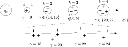
Figure 3: Let $\rho=1$, $q=\infty$ and $d=2$; each vertex has $\mathcaligr{V}=8$ neighbors. Assume potentials satisfy the hypothesis (H), $a(n)\to-\infty$ and the ratio $b(n)/a(n)\to 0$. A copy of $\eta$ occurs on the ball $B(x,r)$. First, the closest local configurations to $\eta_{x}$ are represented according to their number of positive vertices. Thus, the situation of those having $k=3$ positive vertices is specified. The closest ones to $\eta_{x}$ are those having a perimeter $\gamma=18$ and the farthest ones are those having isolated positive vertices, that is, $\gamma=24$.

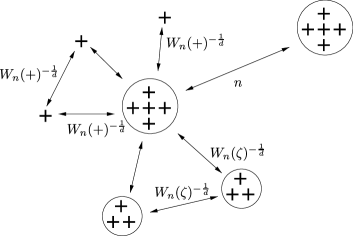
Figure 4: Let $\eta$ be the local configuration having $k(\eta)=5$ positive vertices represented above. Assume potentials $a(n)$ and $b(n)$ satisfy (H). The distance from a given copy of $\eta$ occurring in the graph, say $\eta_{x}$, to its closest positive vertices is of order $W_{n}(+)^{-1/d}$ where $W_{n}(+)$ denotes the weight of a single positive vertex. The distance between such positive vertices is of order $W_{n}(+)^{-1/d}$ too. Let $\zeta$ be the local configuration having $k(\zeta)=3$ positive vertices represented above. The distance from the closest copies of $\zeta$ to $\eta_{x}$ is of order $W_{n}(\zeta)^{-1/d}$ and the distance between such copies is $W_{n}(\zeta)^{-1/d}$ too. Finally, the other copies of $\eta$ occurring in $G_{n}$ are at distance to $\eta_{x}$ of order $n$, since $n^{d}W_{n}(\eta)=\lambda$.

Now, let us consider two copies of a given local configuration $\zeta$ which are at distance to $\eta_{x}$ of order $W_{n}(\zeta)^{-1/d}$. Then, the distance between these two copies necessarily tends to infinity. Otherwise, they would form together a “super” local configuration whose weight would be smaller than $W_{n}(\zeta)$: thanks to Theorem 5.3, such an object would not be at distance to $\eta_{x}$ of order $W_{n}(\zeta)^{-1/d}$. Theorem 5.4 precises this situation. It says the distance between these two copies of $\zeta$ tends to infinity as $W_{n}(\zeta)^{-1/d}$.

Before stating Theorem 5.4, let us introduce the index of $W_{n}$. The hypothesis (H^′) ensures the set $\mathcaligr{D}_{r}(W_{n})$ is nonempty. However, it is not necessary reduced to only one element; it may even contain some local configurations not having the same number of positive vertices. Hence, let us denote by $k_{n}$ and call the index of $W_{n}$ this maximal number:

$$k_{n}=\max_{\zeta\in\mathcaligr{D}_{r}(W_{n})}k(\zeta).$$

Theorem 5.4

Let us consider a local configuration $\eta\in\mathcaligr{C}_{r}$ and potentials $a(n)<0$ and $b(n)\geq 0$ satisfying (H). Let $(R(n))_{n\in\mathbb{N}}$ and $(W_{n})_{n\in\mathbb{N}}$ be two sequences satisfying (H^′). Let $(\ell(n))_{n\in\mathbb{N}}$ be a sequence of integers and $x$ be a vertex. Then,

$$\lim_{n\to+\infty}R(n)W_{n}^{2/d}\max\biggl{\{}\ell(n),\exp\biggl{(}\frac{2}{d}\mathcaligr{V}b(n)k_{n}\biggr{)}\biggr{\}}=0$$

(19)

$$\quad\Longrightarrow\quad\lim_{n\to+\infty}\mu_{a,b}\bigl{(}\mathcaligr{H}_{r}(x,R(n),\ell(n),W_{n})|I_{x}^{\eta}=1\bigr{)}=0;$$

$$\lim_{n\to+\infty}R(n)\ell(n)W_{n}^{2/d}=+\infty$$

(20)

$$\quad\Longrightarrow\quad\lim_{n\to+\infty}\mu_{a,b}\bigl{(}\mathcaligr{H}_{r}(x,R(n),\ell(n),W_{n})|I_{x}^{\eta}=1\bigr{)}=1.$$

Assume a copy of $\eta$ occurs on $B(x,r)$. We know (Theorem 5.3) the distance from $\eta_{x}$ to the closest (copies of) local configurations of weight $W_{n}$ is of order $W_{n}^{-1/d}$. Let us suppose the radius $R(n)$ is of order $W_{n}^{-1/d}$ (i.e., the product $R_{n}^{d}W_{n}$ tends to a positive constant) and let $\zeta_{y}$ be such a copy [i.e., $\zeta\in\mathcaligr{D}_{r}(W_{n})$ occurs on $B(y,r)$ and $\operatorname{dist}(x,y)$ is of order $R(n)$]. If $\ell(n)$ is large compared to $W_{n}^{-1/d}$, then the product $R(n)\ell(n)W_{n}^{2/d}$ tends to infinity and (5.4) says a copy of a local configuration of weight $W_{n}$ can be found at distance from $\zeta_{y}$ smaller than $\ell(n)$. Conversely, if $\ell(n)$ is small compared to $W_{n}^{-1/d}$ then

$$R(n)W_{n}^{2/d}\max\biggl{\{}\ell(n),\exp\biggl{(}\frac{2}{d}\mathcaligr{V}b(n)k_{n}\biggr{)}\biggr{\}}\to 0.$$

Indeed,

$$W_{n}\exp(2\mathcaligr{V}b(n)k_{n}) = W_{n}\exp(-2a(n)k_{n})\exp\bigl{(}2k_{n}\bigl{(}a(n)+\mathcaligr{V}b(n)\bigr{)}\bigr{)}$$

$$\leq \exp\bigl{(}a(n)+\mathcaligr{V}b(n)\bigr{)}$$

by definition of the index $k_{n}$. So, $W_{n}\exp(2\mathcaligr{V}b(n)k_{n})$ tends to $0$ as $n\to+\infty$ thanks to the hypothesis (H). From then on, (5.4) says there is no copy of local configurations of weight $W_{n}$ at distance from $\zeta_{y}$ smaller than $\ell(n)$. Figure 4 represents various local configurations and the distances between each other.

Besides, if the product $R(n)W_{n}^{2/d}$ tends to infinity then (5.4) implies that, at distance from $\eta_{x}$ of order $R(n)$, one can find two copies of local configurations of weight $W_{n}$ so close to each other that we wish. This is not surprising: Theorem 5.3 claims there are local configurations of weight $W_{n}^{2}$ in the ring $\mathcaligr{R}(x,r,R(n))$ provided $R(n)W_{n}^{2/d}\to+\infty$.

Finally, let us underline that Theorems 5.3 and 5.4 would remain unchanged if the radius of local configurations occurring in $\mathcaligr{R}(x,r,R(n))$ might be different from that of $\eta$.

Let us end this section by the following remark. Assume that the local configuration $\eta$ occurs on $B(x,r)$. As long as the ratio $R(n)/n$ tends to $0$, Theorem 5.3 says there is no other copy of $\eta$ in the ring $\mathcaligr{R}(x,r,R(n))$. Now, $n$ represents the size of the graph $G_{n}$. So, if other copies (than $\eta_{x}$) of $\eta$ occur in the graph, they should be at distance of order $n$ from $\eta_{x}$. This is the meaning of Proposition 5.5. Recall that $X_{n}(\eta)$ represents the number of copies of $\eta$ in $G_{n}$. We denote by $\mathcaligr{E}_{n}(\eta)$ the event

$$\exists C>0,(\forall x\not=y,I_{x}^{\eta}=I_{y}^{\eta}=1)\quad\Longrightarrow\quad\operatorname{dist}(x,y)\geq Cn.$$

Proposition 5.5

Let us consider a local configuration $\eta\in\mathcaligr{C}_{r}$ and potentials $a(n)<0$ and $b(n)\geq 0$ satisfying (H). Then,

$$\lim_{n\to+\infty}\mu_{a,b}\bigl{(}\mathcaligr{E}_{n}(\eta)|X_{n}(\eta)\geq 2\bigr{)}=1.$$

Let us recall that the random variable $X_{n}(\eta)$ converges weakly to a Poisson distribution when the hypothesis (H) is satisfied (see Coupier06-2 ). In particular, the fact that no more than one copy of $\eta$ (i.e., $0$ or $1$) occurs in the graph has a positive asymptotic probability. So, conditioning by $X_{n}(\eta)\geq 2$, we avoid this uninteresting case.

5.3 Proofs of Theorems 5.3, 5.4 and Proposition 5.5

The intuition behind Theorem 5.3 is the following. On the one hand, the Markovian character of the Gibbs measure $\mu_{a,b}$ implies that the events $\mathcaligr{A}_{r}(x,R(n),W_{n})$ and $\{I_{x}^{\eta}=1\}$ can be considered as asymptotically independent. So, as $n$ goes to infinity, $\mu_{a,b}(\mathcaligr{A}_{r}(x,R(n),W_{n})|I_{x}^{\eta}=1)$ and $\mu_{a,b}(\mathcaligr{A}_{r}(x,R(n),W_{n}))$ evolve in the same way. On the other hand, the events $\mathcaligr{A}_{r}(x,R(n),W_{n})$ and $\mathcaligr{A}(x,R(n),W_{n})$ (see Section 4) are the same but for a finite number of vertices, those belonging to $B(x,r)$. Their probabilities have the same limit. In conclusion, Theorem 4.1 implies the conditional probability $\mu_{a,b}(\mathcaligr{A}_{r}(x,R(n),W_{n})|I_{x}^{\eta}=1)$ should tend to $0$ or $1$ according to the quantity $R(n)^{d}W_{n}$. The same remarks hold for Theorem 5.4.

Thanks to the invariance translation of the graph $G_{n}$, we only prove Theorems 5.3 and 5.4 for $x=0$ and we will denote, respectively, by $\mathcaligr{A}_{r}(R(n),W_{n})$ and $\mathcaligr{H}_{r}(R(n),\ell(n),W_{n})$ the events $\mathcaligr{A}_{r}(0,R(n),W_{n})$ and $\mathcaligr{H}_{r}(0,R(n),\ell(n),W_{n})$. Let us start with the proof of Theorem 5.3. Proof of Theorem 5.3 Recall the definition of the event $\mathcaligr{A}_{r}(R(n),W_{n})$:

$$\exists y\in\mathcaligr{R}\bigl{(}0,2r,R(n)-r\bigr{)},\exists\zeta\in\mathcaligr{C}_{r}(W_{n})\qquad I_{y}^{\zeta}=1.$$

Let us start with the proof of (5.3). The first step is to move the occurrence of $\zeta$ [the local configuration fulfilling $\mathcaligr{A}_{r}(R(n),W_{n})$] away from the ball $B(0,r)$ on which occurs $\eta$. Let $y$ be a vertex belonging to the ring $\mathcaligr{R}(0,2r,R-r)$. Either $\operatorname{dist}(y,0)\leq 2r+1$ and the ball $B(y,r)$ is included in $\mathcaligr{R}(0,r,3r+1)$. Either $\operatorname{dist}(y,0)>2r+1$ and $B(y,r)$ is included in $\mathcaligr{R}(0,r+1,R(n))$. In other words,

$$\mathcaligr{A}_{r}(R(n),W_{n})\subset\mathcaligr{A}_{r}(3r+1,W_{n})\cup\mathcaligr{A}_{r+1}(R(n),W_{n}).$$ (21)

The hypothesis (H^′) forces the weight $W_{n}$ to be smaller than $\exp(2a(n)-2\mathcaligr{V}b(n))$. Hence, the event $\mathcaligr{A}_{r}(3r+1,W_{n})$ is included in the event $\mathcaligr{A}_{r}(0,3r+1,+)$ introduced in Section 5.1. Lemma 5.1 implies that the conditional probability

$$\mu_{a,b}\bigl{(}\mathcaligr{A}_{r}(3r+1,W_{n})|I_{0}^{\eta}=1\bigr{)}$$

tends to $0$. From (21), it remains to prove the same limit holds for

$$\mu_{a,b}\bigl{(}\mathcaligr{A}_{r+1}(R(n),W_{n})|I_{0}^{\eta}=1\bigr{)}.$$

The strategy consists in introducing increasing events in order to use the FKG inequality. Since $a(n)+\mathcaligr{V}b(n)$ is negative, the following events are both increasing:

$$\bigcup_{\zeta\in\mathcaligr{C}_{r}(W_{n})}\{I_{y}^{\zeta}=1\}\quad\mbox{and}\quad\bigcup_{\eta^{\prime}\in\mathcaligr{C}_{r}(W_{n}(\eta))}\{I_{0}^{\eta^{\prime}}=1\}.$$

So does their intersection

$$S_{y}=\biggl{(}\bigcup_{\zeta\in\mathcaligr{C}_{r}(W_{n})}\{I_{y}^{\zeta}=1\}\biggr{)}\cap\biggl{(}\bigcup_{\eta^{\prime}\in\mathcaligr{C}_{r}(W_{n}(\eta))}\{I_{0}^{\eta^{\prime}}=1\}\biggr{)}.$$

As a consequence, we get from the FKG inequality

$$\quad 1-\mu_{a,b}\bigl{(}\mathcaligr{A}_{r+1}(R(n),W_{n})\cap\{I_{0}^{\eta}=1\}\bigr{)}\geq\prod_{y\in\mathcaligr{R}(0,2r+1,R(n)-r)}\mu_{a,b}(^{c}S_{y}).$$ (22)

Let $y\in\mathcaligr{R}(0,2r+1,R(n)-r)$. Let us denote by $V_{y}$ the union of the two balls $B(y,r)$ and $B(0,r)$, and by $\mathcaligr{C}_{y}$ the set of configurations defined below:

$$\mathcaligr{C}_{y}=\bigl{\{}\omega\in\{-,+\}^{V_{y}},W_{n}\bigl{(}\omega_{B(0,r)}\bigr{)}\leq W_{n}(\eta)\mbox{ and }W_{n}\bigl{(}\omega_{B(y,r)}\bigr{)}\leq W_{n}\bigr{\}}.$$

Then, the probability $\mu_{a,b}(^{c}S_{y})$ becomes

$$\mu_{a,b}(^{c}S_{y})=1-\sum_{\omega\in\mathcaligr{C}_{y}}\mu_{a,b}(I_{V_{y}}^{\omega}=1),$$

where $I_{V_{y}}^{\omega}$ is the random indicator defined on $\mathcaligr{X}_{n}$ as follows: $I_{V_{y}}^{\omega}(\sigma)$ is $1$ if the restriction of the configuration $\sigma\in\mathcaligr{X}_{n}$ to the set $V_{y}$ is $\omega$ and $0$ otherwise. Let $\omega$ be an element of $\mathcaligr{C}_{y}$. Actually, the inequality (7) of Lemma 3.2 can be extended to any subset of vertices $V$ (see Proposition 3.2 of Coupier06-2 ): whenever $a(n)+2\mathcaligr{V}b(n)$ is negative, there exists a constant $C_{V}>0$ such that for all $\omega\in\{-,+\}^{V}$,

$$\mu_{a,b}(I_{V}^{\omega}=1)\leq C_{V}W_{n}(\omega).$$ (23)

Moreover, $C_{V}$ depends on the set $V$ only through its cardinality. Applying (23) to $V=V_{y}$, we obtain

$$\mu_{a,b}(^{c}S_{y})\geq 1-\sum_{\omega\in\mathcaligr{C}_{y}}C_{2,r}W_{n}(\omega),$$

where the constant $C_{2,r}$ only depends on $r$. Now, the condition $\operatorname{dist}(0,y)>2r+1$ forces the connection between the configurations $\omega_{B(0,r)}$ and $\omega_{B(y,r)}$ to be null. Hence, by the identity (3),

$$W_{n}(\omega) = W_{n}\bigl{(}\omega_{B(0,r)}\omega_{B(y,r)}\bigr{)}$$

$$= W_{n}\bigl{(}\omega_{B(0,r)}\bigr{)}W_{n}\bigl{(}\omega_{B(y,r)}\bigr{)}$$

$$\leq W_{n}(\eta)W_{n}.$$

Therefore, for any vertex $y\in\mathcaligr{R}(0,2r+1,R(n)-r)$,

$$\mu_{a,b}(^{c}S_{y})\geq 1-|\mathcaligr{C}_{r}|^{2}C_{2,r}W_{n}(\eta)W_{n}.$$

Hence, coupling this latter lower bound with (22) and Lemma 3.2, it follows that the conditional probability

$$\mu_{a,b}\bigl{(}\mathcaligr{A}_{r+1}(R(n),W_{n})|I_{0}^{\eta}=1\bigr{)}$$

is upper bounded by

$$(c_{r}W_{n}(\eta))^{-1}\bigl{(}1-\bigl{(}1-|\mathcaligr{C}_{r}|^{2}C_{2,r}W_{n}(\eta)W_{n}\bigr{)}^{(2R(n)+1)^{d}}\bigr{)}.$$ (24)

Since the weights $W_{n}$ and $W_{n}(\eta)$ and the product $R(n)^{d}W_{n}$ tend to $0$, (24) is equivalent to

$$2^{d}c_{r}^{-1}|\mathcaligr{C}_{r}|^{2}C_{2,r}R(n)^{d}W_{n}$$

and tends to $0$ as $n$ tends to infinity.

Let us turn to the second part of Theorem 5.3, that is, statement (5.3). Some notation introduced in the previous section will be used here, starting with the set of vertices

$$T_{n}=\biggl{\{}i\bigl{(}\rho(2r+1)+1\bigr{)},|i|=0,\ldots,\biggl{\lfloor}\frac{\rho R(n)}{\rho(2r+1)+1}\biggr{\rfloor}-1\biggr{\}}^{d}\cap B\bigl{(}0,R(n)-r\bigr{)}$$

(see Figure 2). Let $T_{n}^{\ast}=T_{n}\setminus\{0\}$ be the same set without the origin. If $\tau_{n}^{\ast}$ denotes the cardinality of $T_{n}^{\ast}$ then there exists a constant $\tau^{\ast}>0$ such that $\tau_{n}^{\ast}\geq\tau^{\ast}R(n)^{d}$. Let us denote by $\mathcaligr{T}_{n}^{\ast}$ the set

$$\mathcaligr{T}_{n}^{\ast}=\bigcup_{y\in T_{n}^{\ast}}B(y,r)$$

and by $\Gamma_{n}^{\ast}$ the event

$$\Gamma_{n}^{\ast}=\bigcup_{y\in T_{n}^{\ast}}\bigcup_{\zeta\in\mathcaligr{C}_{r}(W_{n})}\{I_{y}^{\zeta}=1\}.$$

The event $\Gamma_{n}^{\ast}$ implies $\mathcaligr{A}_{r}(R(n),W_{n})$. Hence, it suffices to prove that the conditional probability $\mu_{a,b}(^{c}\Gamma_{n}^{\ast}|I_{0}^{\eta}=1)$ tends to $0$. The end of the proof is very close to that of the upper bound of Theorem 4.1, so it will not be detailed.

The balls forming $\mathcaligr{T}_{n}^{\ast}$ are $\mathcaligr{V}$-disjoint. So, by the Property 3.1, the probability $\mu_{a,b}(X_{n}^{\ast}=0\cap I_{0}^{\eta}=1)$ can be expressed as

$$\mathbb{E}_{a,b}\biggl{[}\mu_{a,b}\bigl{(}I_{0}^{\eta}=1|\mathcaligr{F}(\delta B(0,r))\bigr{)}\prod_{y\in T_{n}^{\ast}}\mu_{a,b}\biggl{(}\bigcap_{\zeta\in\mathcaligr{C}_{r}(W_{n})}I_{y}^{\zeta}=0\Big{|}\mathcaligr{F}(\delta B(y,r))\biggr{)}\biggr{]}.$$

Thus, for any vertex $y\in T_{n}^{\ast}$, Lemma 3.2 provides

$$\mu_{a,b}\biggl{(}\bigcap_{\zeta\in\mathcaligr{C}_{r}(W_{n})}I_{y}^{\zeta}=0\Big{|}\mathcaligr{F}(\delta B(y,r))\biggr{)}\leq 1-c_{r}W_{n}.$$

As a consequence,

$$\mu_{a,b}(^{c}\Gamma_{n}^{\ast}\cap I_{0}^{\eta}=1)\leq\mu_{a,b}(I_{0}^{\eta}=1)(1-c_{r}W_{n})^{\tau_{n}^{\ast}}$$

and the conditional probability $\mu_{a,b}(^{c}\Gamma_{n}^{\ast}|I_{0}^{\eta}=1)$ is now controlled:

$$\mu_{a,b}(^{c}\Gamma_{n}^{\ast}|I_{0}^{\eta}=1)\leq\exp(-c_{r}\tau^{\ast}R(n)^{d}W_{n})$$

which tends to $0$ since by hypothesis $R(n)^{d}W_{n}\to+\infty$.

The proof of Theorem 5.4 is based on the same ideas than that of Theorem 5.3. Proof of Theorem 5.4 Recall the definition of $\mathcaligr{H}_{r}(R(n),\ell(n),W_{n})$:

$$\exists y,y^{\prime}\in\mathcaligr{R}\bigl{(}0,2r,R(n)-r\bigr{)},\exists\zeta,\zeta^{\prime}\in\mathcaligr{D}_{r}(W_{n})$$

$$\qquad\mbox{such that }2r<\operatorname{dist}(y,y^{\prime})\leq\ell(n)\quad\mbox{and}\quad I_{y}^{\zeta}=I_{y^{\prime}}^{\zeta^{\prime}}=1.$$

Let us start with the proof of (5.4). The first step consists in moving the occurrences of $\eta$, $\zeta$ and $\zeta^{\prime}$ away from each other. For that purpose, let us introduce the three following events:

$$\mathcaligr{H}^{1}\dvt\exists y\in V_{n},\exists\zeta\in\mathcaligr{D}_{r}(W_{n})\qquad\operatorname{dist}(0,y)=2r+1\quad\mbox{and}\quad I_{y}^{\zeta}=1;$$

$$\mathcaligr{H}^{2}\dvt\exists y,y^{\prime}\in\mathcaligr{R}\bigl{(}0,2r,R(n)-r\bigr{)},\exists\zeta,\zeta^{\prime}\in\mathcaligr{D}_{r}(W_{n})$$

$$\qquad\mbox{such that }\operatorname{dist}(y,y^{\prime})=2r+1\quad\mbox{and}\quad I_{y}^{\zeta}=I_{y^{\prime}}^{\zeta^{\prime}}=1;$$

$$\mathcaligr{H}^{3}\dvt\exists y,y^{\prime}\in\mathcaligr{R}\bigl{(}0,2r+1,R(n)-r\bigr{)},\exists\zeta,\zeta^{\prime}\in\mathcaligr{D}_{r}(W_{n})$$

$$\qquad\mbox{such that }2r+1<\operatorname{dist}(y,y^{\prime})\leq\ell(n)\quad\mbox{and}\quad I_{y}^{\zeta}=I_{y^{\prime}}^{\zeta^{\prime}}=1;$$

whose union contains $\mathcaligr{H}_{r}(R(n),\ell(n),W_{n})$. Thanks to the hypothesis (H^′), $\mathcaligr{H}^{1}$ is included in the event $\mathcaligr{A}_{r}(0,3r+1,+)$ introduced in Section 5.1. So, Lemma 5.1 implies

$$\lim_{n\to+\infty}\mu_{a,b}(\mathcaligr{H}^{1}|I_{0}^{\eta}=1)=0.$$

Let $y,y^{\prime}$ be two vertices such that $\operatorname{dist}(y,y^{\prime})=2r+1$ and $\zeta,\zeta^{\prime}$ be two elements of $\mathcaligr{D}_{r}(W_{n})$ occurring on the balls with radius $r$ centered, respectively, at $y$ and $y^{\prime}$. The convexity of balls forces the connection between $\zeta_{y}$ and $\zeta^{\prime}_{y^{\prime}}$ to be smaller than $\frac{1}{2}\mathcaligr{V}k(\zeta)$. Then, a bound for the weight of the configuration $\zeta_{y}\zeta^{\prime}_{y^{\prime}}$ is deduced:

$$W_{n}(\zeta_{y}\zeta^{\prime}_{y^{\prime}}) = W_{n}(\zeta)W_{n}(\zeta^{\prime})\exp(4b(n)\operatorname{conn}(\zeta_{y},\zeta^{\prime}_{y^{\prime}}))$$

$$\leq W_{n}^{2}\exp(2b(n)\mathcaligr{V}k_{n}),$$

where $k_{n}$ is the index of $W_{n}$. In other words, the event $\mathcaligr{H}^{2}$ implies the existence in the ring $\mathcaligr{R}(0,r,R(n))$ of a local configuration with radius $3r+1$ whose weight is smaller than $W_{n}^{2}\exp(2b(n)\mathcaligr{V}k_{n})$. Now, by hypothesis

$$R(n)^{d}W_{n}^{2}\exp(2b(n)\mathcaligr{V}k_{n})$$

tends to $0$. So, it follows from Theorem 5.3:

$$\lim_{n\to+\infty}\mu_{a,b}(\mathcaligr{H}^{2}|I_{0}^{\eta}=1)=0.$$

It remains to prove the same limit holds for the event $\mathcaligr{H}^{3}$. As at the end of the proof of Theorem 5.3, we are going to introduce increasing events in order to use the FKG inequality. For any vertices $y$, $y^{\prime}$, let us denote by $S_{y,y^{\prime}}$ the event

$$\biggl{(}\bigcup_{\zeta\in\mathcaligr{C}_{r}(W_{n})}\{I_{y}^{\zeta}=1\}\biggr{)}\cap\biggl{(}\bigcup_{\zeta^{\prime}\in\mathcaligr{C}_{r}(W_{n})}\{I_{y^{\prime}}^{\zeta^{\prime}}=1\}\biggr{)}\cap\biggl{(}\bigcup_{\eta^{\prime}\in\mathcaligr{C}_{r}(W_{n}(\eta))}\{I_{0}^{\eta^{\prime}}=1\}\biggr{)}.$$

Since $a(n)+\mathcaligr{V}b(n)$ is negative, $S_{y,y^{\prime}}$ is increasing. Thus, the FKG inequality produces the following lower bound:

$$1-\mu_{a,b}(\mathcaligr{H}^{3}\cap\{I_{0}^{\eta}=1\})\geq\mathop{\mathop{\prod}_{y\in\mathcaligr{R}(0,2r+1,R(n)-r)}}_{y^{\prime}\in\mathcaligr{R}(y,2r+1,\ell(n))}\mu_{a,b}(^{c}S_{y,y^{\prime}}).$$ (25)

Let us pick $y\in\mathcaligr{R}(0,2r+1,R(n)-r)$, $y^{\prime}\in\mathcaligr{R}(y,2r+1,\ell(n))$ and denote by $V_{y,y^{\prime}}$ the union of the three balls $B(y,r)$, $B(y^{\prime},r)$ and $B(0,r)$. Let $\mathcaligr{C}_{y,y^{\prime}}$ be the set of configurations defined by

$$\mathcaligr{C}_{y,y^{\prime}}=\left\{\omega\in\{-,+\}^{V_{y,y^{\prime}}},\⇕⊣⊔∇⟩§{W_{n}\bigl{(}\omega_{B(0,r)}\bigr{)}\leq W_{n}(\eta)\cr W_{n}\bigl{(}\omega_{B(y,r)}\bigr{)}\leq W_{n}\cr W_{n}\bigl{(}\omega_{B(y^{\prime},r)}\bigr{)}\leq W_{n}}\right\}.$$

Then, using inequality (7) of Lemma 3.2 [or rather its extension (23)], we bound the probability of $S_{y,y^{\prime}}$. There exists a constant $C_{3,r}>0$ such that

$$\mu_{a,b}(S_{y,y^{\prime}}) = \sum_{\omega\in\mathcaligr{C}_{y,y^{\prime}}}\mu_{a,b}(I_{V_{y,y^{\prime}}}^{\omega}=1)$$

$$\leq C_{3,r}\sum_{\omega\in\mathcaligr{C}_{y,y^{\prime}}}W_{n}(\omega).$$

Now, vertices $0$, $y$ and $y^{\prime}$ are sufficiently far apart so that the weight of $\omega$ might write as the product of the weights of $\omega_{B(0,r)}$, $\omega_{B(y,r)}$ and $\omega_{B(y^{\prime},r)}$. Then,

$$\mu_{a,b}(S_{y,y^{\prime}})\leq C_{3,r}|\mathcaligr{C}_{r}|^{3}W_{n}(\eta)W_{n}^{2}$$

since $\omega\in\mathcaligr{C}_{y,y^{\prime}}$ and the cardinality of $\mathcaligr{C}_{y,y^{\prime}}$ is bounded by $|\mathcaligr{C}_{r}|^{3}$. Finally, coupling this latter inequality with (25) and Lemma 3.2, we bound the conditional probability $\mu_{a,b}(\mathcaligr{H}^{3}|I_{0}^{\eta}=1)$ by

$$(c_{r}W_{n}(\eta))^{-1}\bigl{(}1-\bigl{(}1-|\mathcaligr{C}_{r}|^{3}C_{3,r}W_{n}(\eta)W_{n}^{2}\bigr{)}^{(2R(n)+1)^{d}(2\ell(n)+1)^{d}}\bigr{)}.$$

Since $W_{n}$, $W_{n}(\eta)$ and the product $\ell(n)^{d}R(n)^{d}W_{n}^{2}$ tend to $0$, the above quantity is equivalent to

$$2^{2d}c_{r}^{-1}|\mathcaligr{C}_{r}|^{3}C_{3,r}\ell(n)^{d}R(n)^{d}W_{n}^{2}$$

and tends to $0$ as $n$ tends to infinity. So does $\mu_{a,b}(\mathcaligr{H}^{3}|I_{0}^{\eta}=1)$.

Let us deal with the second part of Theorem 5.4, that is, statement (5.4).

If the sequence $(\ell(n))_{n\in\mathbb{N}}$ were bounded, say by a constant $\ell(\infty)$, the event $\mathcaligr{H}_{r}(R(n),\ell(n),W_{n})$ would correspond to the existence in the ring $\mathcaligr{R}(0,r,R(n))$ of a local configuration with radius $\ell(\infty)$, say $\zeta$, and whose weight would be larger than $W_{n}^{2}$ [by (3)]. Hence, the limit

$$R(n)^{d}W_{n}(\zeta)\geq\frac{1}{\ell(\infty)^{d}}R(n)^{d}\ell(n)^{d}W_{n}^{2}\to+\infty$$

would imply [statement (5.3) of Theorem 5.3] a limit equal to $1$ for the conditional probability $\mu_{a,b}(\mathcaligr{H}_{r}(R(n),\ell(n),W_{n})|I_{0}^{\eta}=1)$. So, from now on, we will assume that $\ell(n)\to+\infty$.

The second part of Theorem 5.4 needs one more time the set of vertices

$$T_{n}=\biggl{\{}i\bigl{(}\rho(2r+1)+1\bigr{)},|i|=0,\ldots,\biggl{\lfloor}\frac{\rho R(n)}{\rho(2r+1)+1}\biggr{\rfloor}-1\biggr{\}}^{d}\cap B\bigl{(}0,R(n)-r\bigr{)}$$

(see Figure 2). Let $\phi_{n}=i_{n}(\rho(2r+1)+1)$, where

$$i_{n}=\biggl{\lfloor}\frac{\rho({4}/{3}\ell(n)+1)+1}{\rho(2r+1)+1}\biggr{\rfloor}+1,$$

and let us denote by $L_{n}$ the sublattice of $T_{n}$ defined by

$$L_{n}=\bigl{\{}(\phi_{n}\mathbb{Z})^{d}\cap B\bigl{(}0,R(n)-\tfrac{2}{3}\ell(n)\bigr{)}\bigr{\}}\setminus\{0\}.$$

Any two balls $B(y,\frac{2}{3}\ell(n))$ and $B(y^{\prime},\frac{2}{3}\ell(n))$, where $y,y^{\prime}\in L_{n}$, are $\mathcaligr{V}$-disjoint since

$$\operatorname{dist}(y,y^{\prime})\geq\frac{\phi_{n}}{\rho}>\frac{4}{3}\ell(n)+1.$$

Obviously, they are also included in the large ball $B(0,R(n))$. Let us pick a vertex $y$ of $L_{n}$. We denote by $\Lambda_{1}(y)$ and $\Lambda_{2}(y)$ the following subsets of $T_{n}$:

$$\Lambda_{1}(y)=\bigl{\{}z\in T_{n},\operatorname{dist}(z,y)\leq\tfrac{1}{3}\ell(n)\bigr{\}}$$

and

$$\Lambda_{2}(y)=\bigl{\{}z\in T_{n},\tfrac{1}{3}\ell(n)<\operatorname{dist}(z,y)\leq\tfrac{2}{3}\ell(n)\bigr{\}}.$$

Hence, two vertices $z\in\Lambda_{1}(y)$ and $z^{\prime}\in\Lambda_{2}(y)$ satisfy $2r<\operatorname{dist}(z,z^{\prime})\leq\ell(n)$. As a consequence, the event

$$\Gamma=\bigcup_{y\in L_{n}}\mathop{\mathop{\bigcup}_{z\in\Lambda_{1}(y)}}_{z^{\prime}\in\Lambda_{2}(y)}\bigcup_{\zeta,\zeta^{\prime}\in\mathcaligr{D}_{r}(W_{n})}\{I_{z}^{\zeta}=I_{z^{\prime}}^{\zeta^{\prime}}=1\}$$

implies $\mathcaligr{H}_{r}(R(n),\ell(n),W_{n})$. So, it suffices to prove the conditional probability $\mu_{a,b}(^{c}\Gamma|I_{0}^{\eta}=1)$ tends to $0$ as $n\to+\infty$.

The vertices of $\Lambda_{1}(y)$ are the elements of $((\rho(2r+1)+1)\mathbb{Z})^{d}$ whose distance (with respect to $\|\cdot\|_{\infty}$) to $y$ is smaller than $\frac{\rho}{3}\ell(n)$. Their number is of order $\ell(n)^{d}$. More generally, there exists a constant $\alpha$ which depends only on the parameters $d$, $\rho$, $q$ and $r$, such that, for any vertex $y$,

$$|\Lambda_{i}(y)|\geq\alpha\ell(n)^{d},\qquad i=1,2\quad\mbox{and}\quad|L_{n}|\geq\alpha\frac{R(n)^{d}}{\ell(n)^{d}}.$$

Moreover, the Markovian character of the measure $\mu_{a,b}$ (see Property 3.1) allows us to express the probability $\mu_{a,b}(^{c}\Gamma\cap I_{0}^{\eta}=1)$ as the following expectation:

$$\mathbb{E}_{a,b}\biggl{[}\mu_{a,b}\bigl{(}I_{0}^{\eta}=1|\mathcaligr{F}(\delta B(0,r))\bigr{)}$$

$$\qquad{}\times\prod_{y\in L_{n}}\mathop{\mathop{\prod}_{z\in\Lambda_{1}(y)}}_{z^{\prime}\in\Lambda_{2}(y)}\mu_{a,b}\biggl{(}\bigcap_{\zeta,\zeta^{\prime}\in\mathcaligr{D}_{r}(W_{n})}I_{z}^{\zeta}I_{z^{\prime}}^{\zeta^{\prime}}=0\Big{|}\mathcaligr{F}(\delta V_{z,z^{\prime}})\biggr{)}\biggr{]},$$

where $V_{z,z^{\prime}}$ is the union of the two balls $B(z,r)$ and $B(z^{\prime},r)$. Let $y\in L_{n}$ and $z\in\Lambda_{1}(y)$, $z^{\prime}\in\Lambda_{2}(y)$. Let $\sigma\in\{-,+\}^{V_{z,z^{\prime}}}$. Since the balls $B(z,r)$ and $B(z^{\prime},r)$ are $\mathcaligr{V}$-disjoint,

$$\mu_{a,b}\biggl{(}\bigcap_{\zeta,\zeta^{\prime}\in\mathcaligr{D}_{r}(W_{n})}I_{z}^{\zeta}I_{z^{\prime}}^{\zeta^{\prime}}=0\Big{|}\sigma\biggr{)}$$

$$\qquad=1-\sum_{\zeta,\zeta^{\prime}\in\mathcaligr{D}_{r}(W_{n})}\mu_{a,b}\bigl{(}I_{z}^{\zeta}=0|\sigma_{B(z,r)}\bigr{)}\mu_{a,b}\bigl{(}I_{z^{\prime}}^{\zeta^{\prime}}=0|\sigma_{B(z^{\prime},r)}\bigr{)}$$

$$\qquad\leq 1-c_{r}^{2}W_{n}^{2}.$$

In conclusion,

$$\mu_{a,b}(^{c}\Gamma|I_{0}^{\eta}=1) \leq (1-c_{r}^{2}W_{n}^{2})^{\alpha^{3}R(n)^{d}\ell(n)^{d}}$$

$$\leq \exp(-c_{r}^{2}\alpha^{3}R(n)^{d}\ell(n)^{d}W_{n}^{2}),$$

which tends to $0$ whenever $R(n)^{d}\ell(n)^{d}W_{n}^{2}$ tends to $0$.

Let us finish by the proof of Proposition 5.5. It is obtained using the results of the proofs of Lemma 5.1 and Theorem 5.3. Proof of Proposition 5.5 We are going to prove that the quantity $\mu_{a,b}(^{c}\mathcaligr{E}_{n}(\eta)|X_{n}(\eta)\geq 2)$ tends to $0$ as $n\to+\infty$, where the event ${}^{c}\mathcaligr{E}_{n}(\eta)$ means

$$\forall C>0,\exists x\not=y\qquad I_{x}^{\eta}I_{y}^{\eta}=1\quad\mbox{and}\quad\operatorname{dist}(x,y)<Cn.$$

Thanks to the invariance translation of the graph $G_{n}$ and for any constant $C>0$,

$$\mu_{a,b}\bigl{(}^{c}\mathcaligr{E}_{n}(\eta)|X_{n}(\eta)\geq 2\bigr{)}$$

$$\qquad\leq n^{d}\mu_{a,b}\bigl{(}\exists x\not=0,I_{x}^{\eta}I_{0}^{\eta}=1,\operatorname{dist}(x,0)\leq\lfloor Cn\rfloor|X_{n}(\eta)\geq 2\bigr{)}.$$

The condition $X_{n}(\eta)\geq 2$ can be removed. Indeed, the random variable $X_{n}(\eta)$ is asymptotically Poissonian, under the hypothesis (H) (see Coupier06-2 ). So, there exist a constant $\varepsilon>1$ and an integer $n(\varepsilon)$ such that the probability $\mu_{a,b}(X_{n}(\eta)\geq 2)$ is larger than $\varepsilon^{-1}$ whenever $n\geq n(\varepsilon)$. Hence, for such value of $n$,

$$\mu_{a,b}\bigl{(}\exists x\not=0,I_{x}^{\eta}I_{0}^{\eta}=1,\operatorname{dist}(x,0)\leq\lfloor Cn\rfloor|X_{n}(\eta)\geq 2\bigr{)}$$

$$\qquad\leq\varepsilon\mu_{a,b}\bigl{(}\exists x\not=0,I_{x}^{\eta}I_{0}^{\eta}=1,\operatorname{dist}(x,0)\leq\lfloor Cn\rfloor\bigr{)}.$$

In a first time, assume the centers $0$ and $x$ of balls with radius $r$ on which the local configuration $\eta$ occurs satisfy $\operatorname{dist}(x,0)\leq 2r+1$. A configuration of $\{-,+\}^{B(0,R)}$, $R=3r+1$, fulfilling this event necessarily belongs to

$$\mathcaligr{C}_{R}(\eta,+)=\{\zeta\in\mathcaligr{C}_{R},\forall y\in B(0,r),\zeta(y)=\eta(y)\mbox{ and }k(\zeta)>k(\eta)\}.$$

Now, using the inequalities of the proof of Lemma 5.1, we get

$$n^{d}\mu_{a,b}\bigl{(}\exists x\not=0,I_{x}^{\eta}I_{0}^{\eta}=1,\operatorname{dist}(x,0)\leq 2r+1\bigr{)}$$

$$\qquad\leq C_{R}|\mathcaligr{C}_{R}(\eta,+)|n^{d}W_{n}(\eta)\exp(2a(n)),$$

which tends to $0$ since $C_{R}$ and $|\mathcaligr{C}_{R}(\eta,+)|$ are some constants, $n^{d}W_{n}(\eta)=\lambda$ and the magnetic field $a(n)\to-\infty$. So, the case where $\operatorname{dist}(x,0)\leq 2r+1$ is negligible and

$$\limsup_{n\to+\infty}\mu_{a,b}\bigl{(}^{c}\mathcaligr{E}_{n}(\eta)|X_{n}(\eta)\geq 2\bigr{)}$$

$$\qquad\leq\varepsilon\limsup_{n\to+\infty}n^{d}\mu_{a,b}\bigl{(}\exists x\not=0,I_{x}^{\eta}I_{0}^{\eta}=1,2r+1<\operatorname{dist}(x,0)\leq\lfloor Cn\rfloor\bigr{)}$$

for any $C>0$. Remark the event

$$\exists x\not=0\qquad I_{x}^{\eta}I_{0}^{\eta}=1,\qquad 2r+1<\operatorname{dist}(x,0)\leq\lfloor Cn\rfloor$$

is included in $\mathcaligr{A}_{r+1}(0,\lfloor Cn\rfloor,W_{n}(\eta))\cap\{I_{0}^{\eta}=1\}$. The proof of Theorem 5.3 gave us an upper bound for the probability

$$\mu_{a,b}\bigl{(}\mathcaligr{A}_{r+1}(0,\lfloor Cn\rfloor,W_{n}(\eta))\cap\{I_{0}^{\eta}=1\}\bigr{)},$$

which behaves as $\lfloor Cn\rfloor^{d}W_{n}(\eta)^{2}$. Since the product $n^{d}W_{n}(\eta)$ is constant,

$$n^{d}\mu_{a,b}\bigl{(}\exists x\not=0,I_{x}^{\eta}I_{0}^{\eta}=1,2r+1<\operatorname{dist}(x,0)\leq\lfloor Cn\rfloor\bigr{)}$$

is upperbounded by a constant term multiplied by $C^{d}$. Take $C\searrow 0$ and the desired result follows:

$$\limsup_{n\to+\infty}\mu_{a,b}\bigl{(}^{c}\mathcaligr{E}_{n}(\eta)|X_{n}(\eta)\geq 2\bigr{)}=0.$$

6 Ubiquity of local configurations

This section proposes an application of inequalities stated in the proof of Theorem 4.1. Its goal is to give a criterion ensuring that a given local configuration occurs everywhere in the graph. This criterion is presented in Proposition 6.2 through the use of an appropriate Markovian measure built from the Gibbs measure $\mu_{a,b}$ of (2).

A simple way to cover the set of vertices $V_{n}$ by balls consists in using the $L_{\infty}$ norm. In this case, replacing the radius $r$ with $\rho r$, we can assume that $\rho=1$. So, in this section, the neighborhood structure of each vertex is

$$\mathcaligr{V}(x)=\{y\in V_{n},\|y-x\|_{\infty}=1\}.$$

Hence, the graph distance $\mathrm{dist}$ and the $L_{\infty}$ norm define the same sets; the ball $B(x,r)$ is equal to the hypercube with center $x$ and radius $r$.

For all integer $n$, let us denote by $v(n)$ the largest integer $m$ such that $2^{m}$ divides $n$ and by $R(n)$ the integer satisfying the relation

$$\frac{n}{2^{v(n)}}=2R(n)+1.$$

A function $g\dvtx\mathbb{N}^{\ast}\to\mathbb{N}^{\ast}$ satisfying for all integer $n$ the inequalities $v(g(n+1))\geq v(g(n))$ and $R(g(n+1))\geq R(g(n))$, and tending to infinity as $n\to+\infty$ will be said adequate. In particular, an adequate function is nondecreasing. The functions recursively defined by

$$\cases{g(n+1)=2^{v(g(n))+1}\bigl{(}2\bigl{(}R(g(n))+1\bigr{)}+1\bigr{)},&\quad$\forall n\geq 1$,\cr g(1)\in\mathbb{N}^{\ast},}$$

provide examples of adequate functions, since $v(g(n+1))$ and $R(g(n+1))$ are, respectively, equal to $v(g(n))+1$ and $R(g(n))+1$. For instance, if $g(1)=1$ then $g(2)=2^{1}\times 3=6$, $g(3)=2^{2}\times 5=20$, $g(4)=2^{3}\times 7=56,\ldots.$

In conclusion, replacing $n$ with $g(n)$ where $g$ is an adequate function, we will assume that there exists a nondecreasing, integer valued sequence $(R(n))_{n\geq 1}$ such that the sequence

$$\biggl{(}\frac{n}{2R(n)+1}\biggr{)}_{n\geq 1}$$

is nondecreasing and integer valued too.

Now, let us denote by $\tilde{V}_{n}$ the following subset of $V_{n}$:

$$\tilde{V}_{n}=\biggl{\{}i\bigl{(}2R(n)+1\bigr{)},i=0,\ldots,\frac{n}{2R(n)+1}-1\biggr{\}}^{d}.$$

The set of balls $\{B(x,R(n)),x\in\tilde{V}_{n}\}$ is a partition of $V_{n}$. The edge set $\tilde{E}_{n}$ is specified by defining the neighborhood $\tilde{\mathcaligr{V}}(x)$ of each vertex $x\in\tilde{V}_{n}$:

$$\tilde{\mathcaligr{V}}(x)=\{y\in\tilde{V}_{n},\|y-x\|_{\infty}=2R(n)+1\}.$$ (26)

By analogy with the previous sections, we denote by $\delta\tilde{V}$ the neighborhood of $\tilde{V}\subset\tilde{V}_{n}$ corresponding to (26). Hence, an undirected graph structure $\tilde{G}_{n}=(\tilde{V}_{n},\tilde{E}_{n})$ with periodic boundary conditions is defined. The size of $\tilde{G}_{n}$ is the ratio $n$ divided by $2R(n)+1$. Furthermore, remark the graph $\tilde{G}_{n}$ retains the translation invariance property of $G_{n}$.

Let $\eta$ be a local configuration with radius $r$. We associate to $\eta$ a function $f$ from $\mathcaligr{X}_{n}$ into $\tilde{\mathcaligr{X}}_{n}=\{-,+\}^{\tilde{V}_{n}}$ defined for $\sigma\in\mathcaligr{X}_{n}$ and $x\in\tilde{V}_{n}$ by

$$f(\sigma)(x)=+\quad\Longleftrightarrow\quad\exists y\in B(x,R(n))\qquad I_{y}^{\eta}(\sigma)=1.$$

In other words, the vertex $x\in\tilde{V}_{n}$ is positive for the configuration $f(\sigma)\in\tilde{\mathcaligr{X}}_{n}$ if and only if a copy of $\eta$ occurs in the ball $B(x,R(n)+r)$ (under $\sigma$). Remark the function $f$ is onto $\tilde{\mathcaligr{X}}_{n}$. In particular, for $\tilde{V}\subset\tilde{V}_{n}$, the values taken by a configuration $\sigma\in\mathcaligr{X}_{n}$ on the set

$$\Sigma=\bigcup_{y\in\tilde{V}}B\bigl{(}y,R(n)+r\bigr{)}$$

specify completely the configuration $f(\sigma)$ on $\tilde{V}$. Besides, $f$ is not an injective function; for $\zeta\in\{-,+\}^{\tilde{V}}$, $f^{-1}(\zeta)$ represents a subset of $\{-,+\}^{\Sigma}$.

Let $\mathcaligr{F}(\tilde{V})$ be the $\sigma$-algebra generated by the configurations of $\{-,+\}^{\tilde{V}}$. Then, $f^{-1}(\mathcaligr{F}(\tilde{V}))$ is still a $\sigma$-algebra, generated by the sets $f^{-1}(\zeta)$, $\zeta\in\{-,+\}^{\tilde{V}}$, and is coarser than $\mathcaligr{F}(\Sigma)$:

$$f^{-1}(\mathcaligr{F}(\tilde{V}))\varsubsetneq\mathcaligr{F}(\Sigma).$$

Thus, let us endow the set of configurations $\tilde{\mathcaligr{X}}_{n}$ with the measure $\tilde{\mu}_{a,b}$ defined by

$$\forall\zeta\in\tilde{\mathcaligr{X}}_{n}\qquad\tilde{\mu}_{a,b}(\zeta)=\mu_{a,b}(f^{-1}(\zeta)).$$ (27)

Expectations relative to $\tilde{\mu}_{a,b}$ will be denoted by $\tilde{\mathbb{E}}_{a,b}$.

Property 6.1 links the random variable $\tilde{\mu}_{a,b}(\cdot|\mathcaligr{F}(\tilde{V}))$ to $\mu_{a,b}(\cdot|f^{-1}(\mathcaligr{F}(\tilde{V})))$ and states the Markovian character of $\tilde{\mu}_{a,b}$. The identity (28) is completely based on the definition of the measure $\tilde{\mu}_{a,b}$. It holds whatever the function $f$. Relation (29) derives from the Markovian character of the Gibbs measure $\mu_{a,b}$ and the use of the $L_{\infty}$ norm in the construction of the graph $\tilde{G}_{n}$. Property 6.1 will be proved at the end of the section.

Property 6.1

Let $\tilde{U},\tilde{V}$ be two subsets of $\tilde{V}_{n}$. Then, for all event $A\in\mathcaligr{F}(\tilde{U})$,

$$\tilde{\mu}_{a,b}(A|\mathcaligr{F}(\tilde{V}))\circ f=\mu_{a,b}(f^{-1}(A)|f^{-1}(\mathcaligr{F}(\tilde{V}))),$$ (28)

where $\circ$ denotes the composition relation. Moreover, if $\tilde{U}\cap\tilde{V}=\varnothing$ and $\delta\tilde{U}\subset\tilde{V}$ then, for all event $A\in\mathcaligr{F}(\tilde{U})$,

$$\tilde{\mu}_{a,b}(A|\mathcaligr{F}(\tilde{V}))=\tilde{\mu}_{a,b}(A|\mathcaligr{F}(\delta\tilde{U})).$$ (29)

The rest of this section is devoted to the study of the asymptotic behavior of the probability measure $\tilde{\mu}_{a,b}$. As $n$ tends to infinity, the two sequences

$$(R(n))_{n\geq 1}\quad\mbox{and}\quad\biggl{(}\frac{n}{2R(n)+1}\biggr{)}_{n\geq 1}$$

cannot be simultaneously bounded. Then, three alternatives are conceivable; either the graph $G_{n}$ is divided into a small number of large balls, or into a large number of small balls or a large number of large balls.

Proposition 6.2 gives sufficient conditions describing the asymptotic behavior of $\tilde{\mu}_{a,b}$. Relations (30) and (31) are a rewriting of results already known; the second one means at least one copy of the local configuration $\eta$ can be found somewhere in the graph, with probability tending to $1$ (for $\mu_{a,b}$), whenever $W_{n}(\eta)$ is larger than $n^{-d}$. Besides, recall that any given ball $B(x,R(n)+r)$ contains a copy of $\eta$ whenever $W_{n}(\eta)$ is larger than $R(n)^{-d}$ (Theorem 4.1). But, so as to every ball $B(x,R(n)+r)$, $x\in\tilde{V}_{n}$, contains a copy of $\eta$ (this is that we call ubiquity of the local configuration $\eta$) a stronger condition is given by Proposition 6.2; $W_{n}(\eta)$ must be larger than $R(n)^{-d}\ln(n/R(n))$.

For that purpose, let $\zeta_{-}$ and $\zeta_{+}$ be the two configurations of $\tilde{\mathcaligr{X}}_{n}$ whose vertices are all negative and all positive.

Proposition 6.2

Let us consider a local configuration $\eta\in\mathcaligr{C}_{r}$ and potentials $a(n)<0$ and $b(n)\geq 0$ such that $a(n)+2\mathcaligr{V}b(n)\leq 0$.

$$\hskip 22.0pt\mbox{If }\lim_{n\to+\infty}n^{d}W_{n}(\eta)=0\qquad\mbox{then }\lim_{n\to+\infty}\tilde{\mu}_{a,b}(\zeta_{-})=1.$$ (30)

$$\hskip 22.0pt\mbox{If }\lim_{n\to+\infty}n^{d}W_{n}(\eta)=+\infty\qquad\mbox{then }\lim_{n\to+\infty}\tilde{\mu}_{a,b}(\zeta_{-})=0.$$ (31)

$$\hskip 22.0pt\mbox{If }\lim_{n\to+\infty}R(n)^{d}\ln\biggl{(}\frac{n}{R(n)}\biggr{)}^{-1}W_{n}(\eta)=+\infty\qquad\mbox{then }\lim_{n\to+\infty}\tilde{\mu}_{a,b}(\zeta_{+})=1.$$ (32)

Relations (30) and (32), respectively, say that $\tilde{\mu}_{a,b}$ converges weakly to the Dirac measures associated to the configurations $\zeta_{-}$ and $\zeta_{+}$.

The probability (for $\tilde{\mu}_{a,b}$) for a given vertex $x\in\tilde{V}_{n}$ to be positive is equal to the probability (for $\mu_{a,b}$) that the local configuration $\eta$ occurs somewhere in the ball $B(x,R(n)+r)$; see relation (6) below. Now, this quantity has been studied and bounded in Section 4. The proof of Proposition 6.2 immediately derives from this remark. Proof of Proposition 6.2 For $x\in\tilde{V}_{n}$, let $\tilde{I}_{x}^{+}$ be the indicator function defined on $\tilde{\mathcaligr{X}}_{n}$ as follows: $\tilde{I}_{x}^{+}(\zeta)$ is $1$ if the vertex $x$ is positive under $\zeta\in\tilde{\mathcaligr{X}}_{n}$, that is, $\zeta(x)=1$, and $0$ otherwise. Then,

$$\tilde{\mu}_{a,b}(\exists x\in\tilde{V}_{n},\tilde{I}_{x}^{+}=1) = \mu_{a,b}(\exists x\in V_{n},I_{x}^{\eta}=1)$$

$$= \mu_{a,b}\bigl{(}X_{n}(\eta)>0\bigr{)},$$

where $X_{n}(\eta)$ represents the number of copies of $\eta$ occurring in $G_{n}$. In Coupier06-2 , it has been proved that $\mu_{a,b}(X_{n}(\eta)>0)$ tends to $0$ (resp., $1$) whenever $n^{d}W_{n}(\eta)$ tends to $0$ (resp., $+\infty$). Relations (30) and (31) follow.

In order to obtain (32), we are going to prove that the probability of the opposit event $\exists x\in\tilde{V}_{n},\tilde{I}_{x}^{+}=0$ tends to $0$. Due to the translation invariance of $\tilde{G}_{n}$, the random indicators $\tilde{I}_{x}^{+}$ have the same distribution. So,

$$\tilde{\mu}_{a,b}(\exists x\in\tilde{V}_{n},\tilde{I}_{x}^{+}=0)\leq\biggl{(}\frac{n}{R(n)}\biggr{)}^{d}\tilde{\mu}_{a,b}(\tilde{I}_{0}^{+}=0).$$

Furthermore, following the inequalities of the proof of the upper bound of (10), we bound the probability of the event $\tilde{I}_{0}^{+}=0$,

$$\tilde{\mu}_{a,b}(\tilde{I}_{0}^{+}=0) = \mu_{a,b}(\tilde{I}_{0}^{+}\circ f=0)$$

$$= \mu_{a,b}\biggl{(}\sum_{y\in B(0,R(n))}I_{y}^{\eta}=0\biggr{)}$$

$$\leq \exp(-\tau c_{r}R(n)^{d}W_{n}(\eta)),$$

where $\tau$ and $c_{r}$ are positive constant. Finally, (32) is deduced from

$$\tilde{\mu}_{a,b}(\exists x\in\tilde{V}_{n},\tilde{I}_{x}^{+}=0)\leq\exp\biggl{(}-R(n)^{d}W_{n}(\eta)\biggl{(}\tau c_{r}-\frac{d\ln(n/R(n))}{R(n)^{d}W_{n}(\eta)}\biggr{)}\biggr{)}.$$

This section ends with the proof of Property 6.1. Proof of Property 6.1 First, note that any event $A\in\mathcaligr{F}(\tilde{U})$ can be written as a disjoint union of configurations of $\{-,+\}^{\tilde{U}}$. So, it suffices to prove the identities (28) and (29) for $A=\{\zeta\}$, $\zeta\in\{-,+\}^{\tilde{U}}$.

Let us pick such a configuration $\zeta\in\{-,+\}^{\tilde{U}}$. The set $\{f^{-1}(\zeta^{\prime}),\zeta^{\prime}\in\{-,+\}^{\tilde{V}}\}$ is a $\pi$-system which generates the $\sigma$-algebra $f^{-1}(\mathcaligr{F}(\tilde{V}))$. Hence, it is enough to prove

$$\mathbb{E}_{a,b}\bigl{[}\tilde{\mu}_{a,b}(\zeta|\mathcaligr{F}(\tilde{V}))\circ f\mathbh{1}_{f^{-1}(\zeta^{\prime})}\bigr{]}=\mathbb{E}_{a,b}\bigl{[}\mathbh{1}_{f^{-1}(\zeta)}\mathbh{1}_{f^{-1}(\zeta^{\prime})}\bigr{]}$$ (34)

for all $\zeta^{\prime}\in\{-,+\}^{\tilde{V}}$ and

$$\mathbb{E}_{a,b}[\tilde{\mu}_{a,b}(\zeta|\mathcaligr{F}(\tilde{V}))\circ f]=\mathbb{E}_{a,b}\bigl{[}\mathbh{1}_{f^{-1}(\zeta)}\bigr{]}$$ (35)

(see, e.g., Williams , page 84). Let us start with relation (34). For a configuration $\zeta^{\prime}$ belonging to $\{-,+\}^{\tilde{V}}$,

$$\mathbb{E}_{a,b}\bigl{[}\tilde{\mu}_{a,b}(\zeta|\mathcaligr{F}(\tilde{V}))\circ f\mathbh{1}_{f^{-1}(\zeta^{\prime})}\bigr{]} = \mathbb{E}_{a,b}[\tilde{\mu}_{a,b}(\zeta|\mathcaligr{F}(\tilde{V}))\circ f\mathbh{1}_{\zeta^{\prime}}\circ f]$$

$$= \tilde{\mathbb{E}}_{a,b}[\tilde{\mu}_{a,b}(\zeta|\mathcaligr{F}(\tilde{V}))\mathbh{1}_{\zeta^{\prime}}]$$

$$= \tilde{\mathbb{E}}_{a,b}[\mathbh{1}_{\zeta}\mathbh{1}_{\zeta^{\prime}}]$$

$$= \mathbb{E}_{a,b}\bigl{[}\mathbh{1}_{f^{-1}(\zeta)}\mathbh{1}_{f^{-1}(\zeta^{\prime})}\bigr{]}.$$

Relation (35) is treated in the same way:

$$\mathbb{E}_{a,b}[\tilde{\mu}_{a,b}(\zeta|\mathcaligr{F}(\tilde{V}))\circ f] = \tilde{\mathbb{E}}_{a,b}[\tilde{\mu}_{a,b}(\zeta|\mathcaligr{F}(\tilde{V}))]$$

$$= \tilde{\mathbb{E}}_{a,b}[\mathbh{1}_{\zeta}]$$

$$= \mathbb{E}_{a,b}\bigl{[}\mathbh{1}_{f^{-1}(\zeta)}\bigr{]}.$$

Now, let us prove (29) with $A=\{\zeta\}$, $\zeta\in\{-,+\}^{\tilde{U}}$. The set $\{\zeta^{\prime},\zeta^{\prime}\in\{-,+\}^{\delta\tilde{U}}\}$ is a $\pi$-system which generates the $\sigma$-algebra $\mathcaligr{F}(\delta\tilde{U})$. So, since the random variables $\tilde{\mu}_{a,b}(\zeta|\mathcaligr{F}(\tilde{V}))$ and $\tilde{\mu}_{a,b}(\zeta|\mathcaligr{F}(\delta\tilde{U}))$ have the same expectation (equal to $\tilde{\mu}_{a,b}(\zeta)$), it suffices to prove that, for any $\zeta^{\prime}\in\{-,+\}^{\delta\tilde{U}}$,

$$\tilde{\mathbb{E}}_{a,b}[\tilde{\mu}_{a,b}(\zeta|\mathcaligr{F}(\tilde{V}))\mathbh{1}_{\zeta^{\prime}}]=\tilde{\mathbb{E}}_{a,b}[\tilde{\mu}_{a,b}(\zeta|\mathcaligr{F}(\delta\tilde{U}))\mathbh{1}_{\zeta^{\prime}}].$$ (36)

Let $\zeta^{\prime}$ be a configuration of $\{-,+\}^{\delta\tilde{U}}$. First, relation (28) allows us to express the above expectations according to the measure $\mu_{a,b}$:

$$\tilde{\mathbb{E}}_{a,b}[\tilde{\mu}_{a,b}(\zeta|\mathcaligr{F}(\tilde{V}))\mathbh{1}_{\zeta^{\prime}}] = \mathbb{E}_{a,b}[\tilde{\mu}_{a,b}(\zeta|\mathcaligr{F}(\tilde{V}))\circ f\mathbh{1}_{\zeta^{\prime}}\circ f]$$

$$= \mathbb{E}_{a,b}\bigl{[}\mu_{a,b}(f^{-1}(\zeta)|f^{-1}(\mathcaligr{F}(\tilde{V})))\mathbh{1}_{f^{-1}(\zeta^{\prime})}\bigr{]}.$$

Thus, let us denote by $\Sigma_{1}$ and $\Sigma_{2}$ the following sets:

$$\Sigma_{1}=\bigcup_{y\in\delta\tilde{U}}B\bigl{(}y,R(n)+r\bigr{)}\quad\mbox{and}\quad\Sigma_{2}=\biggl{(}\bigcup_{y\in\tilde{V}}B\bigl{(}y,R(n)+r\bigr{)}\biggr{)}\Bigm{\backslash}\Sigma_{1}.$$

Since $f^{-1}(\zeta^{\prime})$ is a subset of $\Sigma_{1}$, we can write

$$\tilde{\mathbb{E}}_{a,b}[\tilde{\mu}_{a,b}(\zeta|\mathcaligr{F}(\tilde{V}))\mathbh{1}_{\zeta^{\prime}}]$$

$$\qquad=\mathop{\mathop{\sum}_{\omega\in\{-,+\}^{\Sigma_{1}}}}_{f(\omega)=\zeta^{\prime}}\mathbb{E}_{a,b}[\mu_{a,b}(f^{-1}(\zeta)|f^{-1}(\mathcaligr{F}(\tilde{V})))\mathbh{1}_{\omega}]$$

$$\qquad=\mathop{\mathop{\sum}_{\omega\in\{-,+\}^{\Sigma_{1}}}}_{f(\omega)=\zeta^{\prime}}\sum_{\omega^{\prime}\in\{-,+\}^{\Sigma_{2}}}\mathbb{E}_{a,b}[\mu_{a,b}(f^{-1}(\zeta)|f^{-1}(\mathcaligr{F}(\tilde{V})))\mathbh{1}_{\omega\omega^{\prime}}],$$

where $\omega\omega^{\prime}$ is a configuration of $\{-,+\}^{\Sigma_{1}\cup\Sigma_{2}}$. Now, the random variable$\mu_{a,b}(f^{-1}(\zeta)|f^{-1}(\mathcaligr{F}(\tilde{V})))$ only depends on the vertices of $\Sigma_{1}\cup\Sigma_{2}$. Hence,

$$\mathbb{E}_{a,b}[\mu_{a,b}(f^{-1}(\zeta)|f^{-1}(\mathcaligr{F}(\tilde{V})))\mathbh{1}_{\omega\omega^{\prime}}]=\mu_{a,b}(f^{-1}(\zeta)|\omega\omega^{\prime})\mu_{a,b}(\omega\omega^{\prime}).$$

Furthermore, the configurations belonging to $f^{-1}(\zeta)$ only depend on the vertices of balls $B(y,R(n)+r)$, $y\in\tilde{U}$, and by construction of the graph $\tilde{G}_{n}$ (and the use of the $L_{\infty}$ norm) the following inclusion holds:

$$\delta\biggl{(}\bigcup_{y\in\tilde{U}}B\bigl{(}y,R(n)+r\bigr{)}\biggr{)}\subset\Sigma_{1}.$$

So, the Markovian character of the measure $\mu_{a,b}$ applies. The conditional probability $\mu_{a,b}(f^{-1}(\zeta)|\omega\omega^{\prime})$ can be reduced to $\mu_{a,b}(f^{-1}(\zeta)|\omega)$ (see Malyshev , page 7). Combining the previous equalities, it follows that

$$\tilde{\mathbb{E}}_{a,b}[\tilde{\mu}_{a,b}(\zeta|\mathcaligr{F}(\tilde{V}))\mathbh{1}_{\zeta^{\prime}}]$$

$$\qquad=\mathop{\mathop{\sum}_{\omega\in\{-,+\}^{\Sigma_{1}}}}_{f(\omega)=\zeta^{\prime}}\mu_{a,b}(f^{-1}(\zeta)|\omega)\sum_{\omega^{\prime}\in\{-,+\}^{\Sigma_{2}}}\mu_{a,b}(\omega\omega^{\prime})$$

$$\qquad=\mathop{\mathop{\sum}_{\omega\in\{-,+\}^{\Sigma_{1}}}}_{f(\omega)=\zeta^{\prime}}\mu_{a,b}(f^{-1}(\zeta)|\omega)\mu_{a,b}(\omega)$$

$$\qquad=\mathop{\mathop{\sum}_{\omega\in\{-,+\}^{\Sigma_{1}}}}_{f(\omega)=\zeta^{\prime}}\mathbb{E}_{a,b}[\mu_{a,b}(f^{-1}(\zeta)|f^{-1}(\mathcaligr{F}(\delta\tilde{U})))\mathbh{1}_{\omega}]$$

$$\qquad=\mathbb{E}_{a,b}\bigl{[}\mu_{a,b}(f^{-1}(\zeta)|f^{-1}(\mathcaligr{F}(\delta\tilde{U})))\mathbh{1}_{f^{-1}(\zeta^{\prime})}\bigr{]}.$$

Finally, using a second time the relation (28), we get the desired identity:

$$\tilde{\mathbb{E}}_{a,b}[\tilde{\mu}_{a,b}(\zeta|\mathcaligr{F}(\tilde{V}))\mathbh{1}_{\zeta^{\prime}}] = \mathbb{E}_{a,b}[\tilde{\mu}_{a,b}(\zeta|\mathcaligr{F}(\delta\tilde{U}))\circ f\mathbh{1}_{\zeta^{\prime}}\circ f]$$

$$= \tilde{\mathbb{E}}_{a,b}[\tilde{\mu}_{a,b}(\zeta|\mathcaligr{F}(\delta\tilde{U}))\mathbh{1}_{\zeta^{\prime}}].$$

References

- (1) {barticle}[mr] \bauthor\bsnmAbadi, \bfnmM.\binitsM., \bauthor\bsnmChazottes, \bfnmJ.-R.\binitsJ.-R., \bauthor\bsnmRedig, \bfnmF.\binitsF. and \bauthor\bsnmVerbitskiy, \bfnmE.\binitsE. (\byear2004). \btitleExponential distribution for the occurrence of rare patterns in Gibbsian random fields. \bjournalComm. Math. Phys. \bvolume246 \bpages269–294. \bidmr=2048558 \endbibitem
- (2) {barticle}[mr] \bauthor\bsnmAbadi, \bfnmM.\binitsM. and \bauthor\bsnmGalves, \bfnmA.\binitsA. (\byear2001). \btitleInequalities for the occurrence times of rare events in mixing processes. The state of the art. \bjournalMarkov Process. Related Fields \bvolume7 \bpages97–112. \bidmr=1835750\endbibitem
- (3) {bbook}[mr] \bauthor\bsnmBarbour, \bfnmA. D.\binitsA. D., \bauthor\bsnmHolst, \bfnmLars\binitsL. and \bauthor\bsnmJanson, \bfnmSvante\binitsS. (\byear1992). \btitlePoisson Approximation. \bseriesOxford Studies in Probability \bvolume2. \bpublisherOxford Univ. Press, \baddressNew York. \bidmr=1163825 \endbibitem
- (4) {bbook}[mr] \bauthor\bsnmBollobás, \bfnmBéla\binitsB. (\byear1985). \btitleRandom Graphs. \bpublisherAcademic Press, \baddressLondon. \bidmr=809996 \endbibitem
- (5) {barticle}[mr] \bauthor\bsnmBoppona, \bfnmRavi\binitsR. and \bauthor\bsnmSpencer, \bfnmJoel\binitsJ. (\byear1989). \btitleA useful elementary correlation inequality. \bjournalJ. Combin. Theory Ser. A \bvolume50 \bpages305–307. \bidmr=989201 \endbibitem
- (6) {barticle}[mr] \bauthor\bsnmChazottes, \bfnmJ.-R.\binitsJ.-R. and \bauthor\bsnmRedig, \bfnmF.\binitsF. (\byear2005). \btitleOccurrence, repetition and matching of patterns in the low-temperature Ising model. \bjournalJ. Stat. Phys. \bvolume121 \bpages579–605. \bidmr=2185340 \endbibitem
- (7) {barticle}[mr] \bauthor\bsnmChen, \bfnmLouis H. Y.\binitsL. H. Y. (\byear1975). \btitlePoisson approximation for dependent trials. \bjournalAnn. Probab. \bvolume3 \bpages534–545. \bidmr=0428387 \endbibitem
- (8) {bmisc}[auto:springertagbib-v1.0] \bauthor\bsnmCoupier, \bfnmD.\binitsD. (\byear2005). \btitleAsymtotique des propriétés locales pour le modèle d’ising et applications. Ph.D. thesis, Univ. Paris 5. \endbibitem
- (9) {barticle}[mr] \bauthor\bsnmCoupier, \bfnmD.\binitsD. (\byear2006). \btitlePoisson approximations for the Ising model. \bjournalJ. Stat. Phys. \bvolume123 \bpages473–495. \bidmr=2227091 \endbibitem
- (10) {barticle}[mr] \bauthor\bsnmCoupier, \bfnmDavid\binitsD. (\byear2008). \btitleTwo sufficient conditions for Poisson approximations in the ferromagnetic Ising model. \bjournalAnn. Appl. Probab. \bvolume18 \bpages1326–1350. \bidmr=2434173 \endbibitem
- (11) {barticle}[mr] \bauthor\bsnmCoupier, \bfnmDavid\binitsD., \bauthor\bsnmDoukhan, \bfnmPaul\binitsP. and \bauthor\bsnmYcart, \bfnmBernard\binitsB. (\byear2006). \btitleZero-one laws for binary random fields. \bjournalALEA Lat. Am. J. Probab. Math. Stat. \bvolume2 \bpages157–175. \bidmr=2249667 \endbibitem
- (12) {barticle}[mr] \bauthor\bsnmErdős, \bfnmP.\binitsP. and \bauthor\bsnmRényi, \bfnmA.\binitsA. (\byear1960). \btitleOn the evolution of random graphs. \bjournalMagyar Tud. Akad. Mat. Kutató Int. Közl. \bvolume5 \bpages17–61. \bidmr=0125031 \endbibitem
- (13) {barticle}[mr] \bauthor\bsnmFernández, \bfnmRoberto\binitsR., \bauthor\bsnmFerrari, \bfnmPablo A.\binitsP. A. and \bauthor\bsnmGarcia, \bfnmNancy L.\binitsN. L. (\byear2001). \btitleLoss network representation of Peierls contours. \bjournalAnn. Probab. \bvolume29 \bpages902–937. \bidmr=1849182 \endbibitem
- (14) {barticle}[auto:springertagbib-v1.0] \bauthor\bsnmFerrari, \bfnmP. A.\binitsP. A. and \bauthor\bsnmPicco, \bfnmP.\binitsP. (\byear2000). \btitlePoisson approximation for large-contours in low-temperature Ising models. \bjournalPhys. A \bvolume279 \bpages303–311. \endbibitem
- (15) {barticle}[mr] \bauthor\bsnmFortuin, \bfnmC. M.\binitsC. M., \bauthor\bsnmKasteleyn, \bfnmP. W.\binitsP. W. and \bauthor\bsnmGinibre, \bfnmJ.\binitsJ. (\byear1971). \btitleCorrelation inequalities on some partially ordered sets. \bjournalComm. Math. Phys. \bvolume22 \bpages89–103. \bidmr=0309498 \endbibitem
- (16) {barticle}[mr] \bauthor\bsnmGanesh, \bfnmA.\binitsA., \bauthor\bsnmHambly, \bfnmB. M.\binitsB. M., \bauthor\bsnmO’Connell, \bfnmNeil\binitsN., \bauthor\bsnmStark, \bfnmDudley\binitsD. and \bauthor\bsnmUpton, \bfnmP. J.\binitsP. J. (\byear2000). \btitlePoissonian behavior of Ising spin systems in an external field. \bjournalJ. Stat. Phys. \bvolume99 \bpages613–626. \bidmr=1762669 \endbibitem
- (17) {bbook}[mr] \bauthor\bsnmGeorgii, \bfnmHans-Otto\binitsH.-O. (\byear1988). \btitleGibbs Measures and Phase Transitions. \bseriesDe Gruyter Studies in Mathematics \bvolume9. \bpublisherDe Gruyter, \baddressBerlin. \bidmr=956646 \endbibitem
- (18) {bbook}[mr] \bauthor\bsnmGrimmett, \bfnmGeoffrey\binitsG. (\byear1989). \btitlePercolation. \bpublisherSpringer, \baddressNew York. \bidmr=995460 \endbibitem
- (19) {barticle}[mr] \bauthor\bsnmJanson, \bfnmSvante\binitsS. (\byear1990). \btitlePoisson approximation for large deviations. \bjournalRandom Structures Algorithms \bvolume1 \bpages221–229. \bidmr=1138428 \endbibitem
- (20) {bincollection}[mr] \bauthor\bsnmJanson, \bfnmSvante\binitsS., \bauthor\bsnmŁuczak, \bfnmTomasz\binitsT. and \bauthor\bsnmRuciński, \bfnmAndrzej\binitsA. (\byear1990). \btitleAn exponential bound for the probability of nonexistence of a specified subgraph in a random graph. In \bbooktitleRandom Graphs ’87 (Poznań, 1987) \bpages73–87. \bpublisherWiley, \baddressChichester. \bidmr=1094125 \endbibitem
- (21) {bbook}[mr] \bauthor\bsnmKindermann, \bfnmRoss\binitsR. and \bauthor\bsnmSnell, \bfnmJ. Laurie\binitsJ. L. (\byear1980). \btitleMarkov Random Fields and Their Applications. \bseriesContemporary Mathematics \bvolume1. \bpublisherAmer. Math. Soc., \baddressProvidence, RI. \bidmr=620955 \endbibitem
- (22) {bbook}[mr] \bauthor\bsnmMalyshev, \bfnmV. A.\binitsV. A. and \bauthor\bsnmMinlos, \bfnmR. A.\binitsR. A. (\byear1991). \btitleGibbs Random Fields. \bseriesMathematics and Its Applications \bvolume44. \bpublisherKluwer Academic, \baddressDordrecht. \bidmr=1191166 \endbibitem
- (23) {bbook}[mr] \bauthor\bsnmSpencer, \bfnmJoel\binitsJ. (\byear2001). \btitleThe Strange Logic of Random Graphs. \bseriesAlgorithms and Combinatorics \bvolume22. \bpublisherSpringer, \baddressBerlin. \bidmr=1847951 \endbibitem
- (24) {bbook}[mr] \bauthor\bsnmWilliams, \bfnmDavid\binitsD. (\byear1991). \btitleProbability with Martingales. \bpublisherCambridge Univ. Press, \baddressCambridge. \bidmr=1155402 \endbibitem