Frictional quantum decoherence

Abstract

The dynamics associated with a measurement-based master equation for quantum Brownian motion are investigated. A scheme for obtaining time evolution from general initial conditions is derived. This is applied to analyze dissipation and decoherence in the evolution of both a Gaussian and a Schrödinger cat initial state. Dependence on the diffusive terms present in the master equation is discussed with reference to both the coordinate and momentum representations.

1 Introduction

The connection between quantum dissipation and decoherence is a topic of longstanding interest [1, 2, 3, 4, 5, 6, 7, 8, 9]. The main systems analyzed in this perspective are the damped harmonic oscillator, two level systems and quantum Brownian motion. For such systems the Hamiltonian description is not appropriate, and the most successful results come from the reduced description of a particle interacting with some type of reservoir [10]. Classical understanding of the phenomenon is well-established, relying on Langevin or Fokker-Planck equations obtained by considering a particle interacting with a bath of independent oscillators [11]. The quantum counterpart of classical Brownian motion, however, has only recently been cast into standard equations [12, 13].

Several approaches have been followed in order to obtain a quantum description of the dynamics of the Brownian particle:

• a model-reservoir approach, leading to the famous Caldeira and Leggett master equation, which assumes the particle to be coupled to an environment described by a collection of simple harmonic oscillators [1, 2], and into which suitable terms can be added in order to produce a satisfactory Markovian equation of the required Lindblad form [3, 4],

• a dynamical approach modelling more closely the random collisions between the Brownian particle and the particles that make up its surrounding environment [5, 6, 7],

• a measurement-based approach focusing on the information about the Brownian particle carried away by the particles of the medium during the collisions. This information is available, at least in principle, by monitoring the environment particles [8, 9, 12, 13].

The property of complete positivity, to be satisfied by a master equation for the reduced density operator of the particle, is a useful and stringent requirement in the study of subdynamics in quantum mechanics [14]. The various approaches are described in [12], where the results obtained with the different methods are discussed. Of particular relevance is whether or not the proposed master equations are Markovian and of Lindblad form.

Here the approach that we use to describe the quantum Brownian particle dynamics is the measurement-based one found in [12, 13, 15]. The collisions with the surrounding particles are considered to perform a random sequence of measurements feeding information about the position and momentum of the Brownian particle into the environment. Even if both of these quantities cannot be known with total precision at the same time, it is possible to simultaneously measure position and momentum by introducing some degree of imprecision for both. Using non-quantum-limited measurement techniques to represent the acquisition of this information [16] has led to the following master equation, in the limit of frequent collisions which make very weak joint measurements of position and momentum [12]:

$$\frac{\mathrm{d}\hat{\rho}}{\mathrm{d}t}=-\frac{i}{\hbar}\left[\frac{{\hat{p}}^{2}}{2M},\hat{\rho}\right]-\frac{i\gamma}{2\hbar}\left[\hat{x},\{\hat{p},\hat{\rho}\}\right]-\frac{D_{pp}}{\hbar^{2}}\left[\hat{x},[\hat{x},\hat{\rho}]\right]-\frac{D_{xx}}{\hbar^{2}}\left[\hat{p},[\hat{p},\hat{\rho}]\right]\,.$$ (1)

This equation is of the required Lindblad form provided that

$$D_{pp}D_{xx}\geq(\hbar\gamma/4)^{2}\,.$$ (2)

Here $M$ is the mass of the Brownian particle, $\gamma$ is the damping coefficient while $D_{pp}$ and $D_{xx}$ are diffusion coefficients given by

$$D_{pp}=\gamma\left[Mk_{B}T+\frac{m}{M}{(\Delta_{\sigma}p)}^{2}\right]+\frac{R\hbar^{2}}{8{(\Delta_{\sigma}x)}^{2}}\,,$$ (3)

and

$$D_{xx}=\frac{R\hbar^{2}}{8{(\Delta_{\sigma}p)}^{2}}\,.$$ (4)

The particles forming the environment have mass $m$, $R$ is the average rate of collisions and $\Delta_{\sigma}p$ and $\Delta_{\sigma}x$ represent the increase in the standard deviations due to the measurements of position and momentum over and above the intrinsic variances [12].

Satisfaction of the condition of Eq. (2) using Eq. (3) and (4) ensures that the master equation is of Lindblad form. The existence of analogous master equations obtained by other approaches, but with different expressions for $D_{pp}$ and $D_{xx}$ [9, 10], has been described in [12]. The Caldeira-Leggett master equation [1], is Markovian but is not of Lindblad form and this has been shown to lead to serious difficulties including, in particular, negative probabilities [17, 18, 13]. These problems do not arise for Eq. (1) because of the presence in $D_{pp}$ of two new terms other than the temperature dependent one, $\gamma Mk_{B}T$. These depend on the variances $\Delta_{\sigma}p$ and $\Delta_{\sigma}x$, and in particular the presence of a new double commutator term representing a position diffusion regulated by $D_{xx}$. The origin of these terms is the inherent spreading in position(momentum) which occurs when a measurement of momentum(position) is made. This point has been discussed further in [13].

The main aim of this paper is an analysis of the decoherence dynamics associated with Eq. (1). In particular we find the exact solution of the master equation, and then use this to illuminate the role of both the $D_{pp}$ and the hitherto largely unconsidered $D_{xx}$ terms in dissipation and decoherence. To this end we will consider two initial states for the Brownian particle: a single Gaussian wave packet and Schrödinger cat state. By way of comparison we also consider cases where $D_{pp}$ and $D_{xx}$, can be varied independently, which can, for example, furnish the Caldeira-Leggett dynamics when $D_{pp}=\gamma Mk_{B}T$ and $D_{xx}=0$.

The paper is organized as follows. In Sec. 2 we solve the master equation, providing a general scheme for obtaining time evolution from general initial conditions. In Sec. 3 we apply this scheme to two initial configurations, and discuss their dynamical evolution. In Sec. 4 we consider briefly what happens when the Lindblad condition given by Eq. (2) is not satisfied. In Sec. 5 we summarize and discuss our results. In A and B we collect some of the lengthier calculations.

2 Solution of the master equation

In this section we solve the master equation by introducing a characteristic function. This procedure has been previously used to obtain a formal solution of the Caldeira-Leggett master equation, and is described, for example, in [19]. The main difference here is that there is an additional term depending on the position diffusion $D_{xx}$.

In the position representation Eq. (1) takes the form:

$$\!\!\!\!\!\!\!\!\!\!\!\!\!\!\!\!\!\frac{\partial\rho(x,x^{\prime},t)}{\partial t}= \left[\frac{i\hbar}{2M}\left(\frac{\partial^{2}}{\partial x^{2}}-\frac{\partial^{2}}{\partial x^{\prime 2}}\right)-\frac{i\gamma}{2}(x-x^{\prime})\left(\frac{\partial}{\partial x}-\frac{\partial}{\partial x^{\prime}}\right)-\frac{D_{pp}}{\hbar^{2}}(x-x^{\prime})^{2}\right.$$ (5)

$$-\left.D_{xx}\left(\frac{\partial^{2}}{\partial x^{2}}+\frac{\partial^{2}}{\partial x^{\prime 2}}-2\frac{\partial}{\partial x}\frac{\partial}{\partial x^{\prime}}\right)\right]\rho(x,x^{\prime},t)\,,$$

where $\rho(x,x^{\prime},t)=\langle x|\rho|x^{\prime}\rangle$. This second order linear partial differential equation can be greatly simplified by moving to a ($k,\Delta_{t}$) representation [20] based on introducing the characteristic function $\rho(k,\Delta_{t},t)$:

$$\rho(k,\Delta_{t},t)=\mathrm{tr}(\hat{D}\hat{\rho})=\mathrm{tr}(\exp[i(k\hat{x}+\Delta_{t}\hat{p})]\hat{\rho})=\int_{-\infty}^{+\infty}\!\!\mathrm{d}x\,\mathrm{e}^{ikx}\rho\left(x+\frac{\hbar\Delta_{t}}{2},x-\frac{\hbar\Delta_{t}}{2},t\right).$$ (6)

In this new representation we obtain a first order partial differential equation in the form

$$\!\!\!\!\!\!\!\!\frac{\partial\rho(k,\Delta_{t},t)}{\partial t}=\left[\frac{k}{M}\frac{\partial}{\partial\Delta_{t}}-\gamma\Delta_{t}\frac{\partial}{\partial\Delta_{t}}-D_{pp}\Delta^{2}_{t}-D_{xx}k^{2}\right]\rho(k,\Delta_{t},t)\,.$$ (7)

In A the method of characteristics [21] is used to solve this partial differential equation exactly. The solution is

$$\rho(k,\Delta_{t},t)=\rho\left(k,\Delta_{t}(1-\Gamma)+\frac{k}{\gamma M}\Gamma,0\right)\times$$

$$\exp\left\{\left[-\left(D_{xx}+\frac{D_{pp}}{M^{2}\gamma^{2}}\right)t+\frac{D_{pp}}{M^{2}\gamma^{3}}\left(\frac{\Gamma^{2}}{2}+\Gamma\right)\right]k^{2}-\frac{D_{pp}\Gamma^{2}}{M\gamma^{2}}k\Delta_{t}-\frac{D_{pp}\Gamma(2-\Gamma)}{2\gamma}\Delta_{t}^{2}\,\right\},$$ (8)

where $\Delta_{0}=\Delta_{t}(1-\Gamma)+\frac{k}{\gamma M}\Gamma$ and $\Gamma=1-\exp(-\gamma t)$.

We can use Eq. (6) and its inverse to move to and from the coordinate and $(k,\Delta_{t})$ representations at will, and Eq. (2) to obtain the time evolution in the $(k,\Delta_{t})$ representation. This allows us to compute the time evolution of a general initial state in the position representation by following the procedure:

$$\rho(x,x^{\prime},0)\rightarrow\rho(k,\Delta_{0},0)\rightarrow\rho(k,\Delta_{t},t)\rightarrow\rho(x,x^{\prime},t)\,.$$ (9)

In the next section we will use this procedure to solve the master equation for two initial states which can be written in the coordinate representation as a sum of exponential terms of the form

$$\rho(x,x^{\prime},0)= \exp\left[-A_{0}(x-x^{\prime})^{2}-iB_{0}(x-x^{\prime})(x+x^{\prime})\right.$$ (10)

$$\left.-C_{0}(x+x^{\prime})^{2}-iD_{0}(x-x^{\prime})-E_{0}(x+x^{\prime})-F_{0}\right]\,.$$

We here apply the scheme outlined by Eq. (9) to obtain the time evolution for states of this kind. Using Eqs. (6) and (2) we find the characteristic function at time $t$ in the $(k,\Delta_{t})$ representation to be

$$\rho(k,\Delta_{t},t)=\exp\left[-a_{t}k^{2}-ib_{t}k\Delta_{t}-c_{t}\Delta^{2}_{t}-id_{t}k-ie_{t}\Delta_{t}-f_{t}\right]\,,$$ (11)

where the various coefficients follow the time evolution given by

$$a_{t} = a_{0}+b_{0}\frac{\Gamma}{M\gamma}+c_{0}\left(\frac{\Gamma}{M\gamma}\right)^{2}+\left(D_{xx}+\frac{D_{pp}}{M^{2}\gamma^{2}}\right)t-\frac{D_{pp}}{M^{2}\gamma^{3}}\left(\frac{\Gamma^{2}}{2}+\Gamma\right),$$

$$b_{t} = b_{0}(1-\Gamma)+c_{0}\frac{2\Gamma(1-\Gamma)}{M\gamma}+\frac{D_{pp}\Gamma^{2}}{M\gamma^{2}},\quad c_{t}=c_{0}(1-\Gamma)^{2}+\frac{D_{pp}\Gamma(2-\Gamma)}{2\gamma},$$

$$d_{t} = d_{0}+e_{0}\frac{\Gamma}{M\gamma},\quad e_{t}=e_{0}(1-\Gamma),\quad f_{t}=f_{0}\,,$$ (12)

and where the relation between small and capital coefficients is given by

$$a_{0}=\frac{1}{16C_{0}},\,\,\,b_{0}=-\frac{B_{0}}{4C_{0}}\hbar,\,\,\,c_{0}=\frac{4A_{0}C_{0}+B_{0}^{2}}{4C_{0}}\hbar^{2},\quad d_{0}=\frac{E_{0}}{4C_{0}}$$

$$e_{0}=\frac{2C_{0}D_{0}-B_{0}E_{0}}{2C_{0}}\hbar,\quad\exp(-f_{0})=\exp(-F_{0})\exp\left(-\frac{E_{0}^{2}}{4C_{0}}\right)\frac{1}{2}\sqrt{\frac{\pi}{C_{0}}}\,.$$ (13)

Transformation back to the coordinate representation Eq. (11) provides the density matrix

$$\rho(x,x^{\prime},t)= \exp\left[-A_{t}(x-x^{\prime})^{2}-iB_{t}(x-x^{\prime})(x+x^{\prime})\right.$$ (14)

$$\left.-C_{t}(x+x^{\prime})^{2}-iD_{t}(x-x^{\prime})-E_{t}(x+x^{\prime})-F_{t}\right]\,,$$

with the following relationships

$$A_{t}=\frac{4a_{t}c_{t}-b_{t}^{2}}{4\hbar^{2}a_{t}},\quad B_{t}=-\frac{b_{t}}{4\hbar a_{t}},\quad C_{t}=\frac{1}{16a_{t}},\quad D_{t}=\frac{2a_{t}e_{t}-b_{t}d_{t}}{2\hbar a_{t}},$$ (15)

$$E_{t}=\frac{d_{t}}{4a_{t}},\quad\exp(-F_{t})=\frac{\exp(-f_{t})}{2\sqrt{\pi a_{t}}}\exp\left(-\frac{d_{t}^{2}}{4a_{t}}\right)\,.$$

The inverse relations can also be found:

$$a_{t}=\frac{1}{16C_{t}},\,\,\,b_{t}=-\frac{B_{t}}{4C_{t}}\hbar,\,\,\,c_{t}=\frac{4A_{t}C_{t}+B_{t}^{2}}{4C_{t}}\hbar^{2},\quad d_{t}=\frac{E_{t}}{4C_{t}}$$

$$e_{t}=\frac{2C_{t}D_{t}-B_{t}E_{t}}{2C_{t}}\hbar,\quad\exp(-f_{t})=\exp(-F_{t})\exp\left(-\frac{E_{t}^{2}}{4C_{t}}\right)\frac{1}{2}\sqrt{\frac{\pi}{C_{t}}}\,.$$ (16)

For density matrices which correspond to superpositions of states centred on different positions, each of which is individually of the form given by Eq. (10), the linearity of Eq. (7) means that it is still possible to follow the procedure described by Eq. (9) and so to compute the time evolution.

3 Applications

In this section we consider two physically interesting initial states, the simple Gaussian wavepacket and a superposition of two such states, which forms a Schrödinger cat state. Using the procedure described in the preceding section to compute their time evolution, we focus on the role of the momentum and position diffusion terms, proportional to $D_{pp}$ and $D_{xx}$ respectively. In particular many of our results will be expressed in terms of these coefficients and will not depend on their explicit form [Eqs. (3) and (4)] in terms of the physical parameters of the system. These results have a general validity, therefore for any master equation with the same form as Eq. (1) irrespective of the sizes of the diffusion terms. Thus our method does not just provide the solution to Eq. (1), but also an infinity of other master equations whose diffusion terms do not necessarily satisfy the Lindblad condition (Eq. (2)). One particular example is the Caldeira-Leggett master equation obtained by putting $D_{pp}=\gamma Mk_{B}T$ and $D_{xx}=0$.

3.1 Single Gaussian wave packet

Consider a minimum uncertainty Gaussian wave packet centered at position $x_{0}=0$ and momentum $p_{0}$, with initial spreads in position and momentum ${\Delta x}_{0}$ and ${\Delta p}_{0}$ which satisfy the uncertainty principle ${\Delta x}_{0}{\Delta p}_{0}=\frac{\hbar}{2}$,

$$\rho(x,x^{\prime},0)=\frac{1}{\sqrt{2\pi{\Delta x}_{0}^{2}}}\exp\left[-\frac{(x-x^{\prime})^{2}}{8{\Delta x}_{0}^{2}}-\frac{(x+x^{\prime})^{2}}{8{\Delta x}_{0}^{2}}+i\frac{p_{0}(x-x^{\prime})}{\hbar}\right]\,.$$ (17)

By comparing this initial reduced density matrix with Eq. (10) at $t=0$ we can identify the required coefficients as

$$A_{0}=C_{0}=\frac{1}{8{\Delta x}_{0}^{2}},\quad B_{0}=E_{0}=0,\quad D_{0}=-\frac{p_{0}}{\hbar},\quad\exp(-F_{0})=\frac{1}{\sqrt{2\pi{\Delta x}_{0}^{2}}}\,.$$ (18)

By using Eq. (6) we can obtain the corresponding initial condition in the ($k,\Delta_{t}$) representation, which has the exponential form of Eq. (11) for $t=0$ with

$$a_{0}=\frac{{{\Delta x}_{0}}^{2}}{2},\quad b_{0}=0,\quad c_{0}=\frac{{{\Delta p}_{0}}^{2}}{2},\quad d_{0}=0,\quad e_{0}=-p_{0},\quad f_{0}=0\,.$$ (19)

¿From Eq. (2) we next compute the time evolution of the various coefficients, and then return to the coordinate representation using Eqs. (14) and (15). Thus we obtain the spatial reduced density matrix at time $t$, from which it is also possible to obtain the corresponding density matrix in the momentum representation by double Fourier transformation. The solution provides a simple means of obtaining the time evolution of the average of $\hat{x}$ and $\hat{p}$, and of their variances shown below and plotted in Fig. 1 for physically reasonable parameter values,

$$\langle\hat{x}\rangle_{t} = -d_{t},\,\,\,\langle\hat{p}\rangle_{t}=-e_{t},\,\,\,{\Delta x}^{2}_{t}=2a_{t},\,\,\,{\Delta p}^{2}_{t}=2c_{t}\,.$$ (20)

These equations could equally well be rewritten in terms of the capitalized coefficients using Eq. (2), but the evolution is given most simply in terms of the initial conditions using Eq. (2). The expectation values become

$$\langle\hat{x}\rangle_{t}=\frac{p_{0}}{M}\frac{1-\exp(-\gamma t)}{\gamma},\quad\langle\hat{p}\rangle_{t}=p_{0}\exp(-\gamma t),\quad{\Delta x}^{2}_{t}={\Delta x}^{2}_{0}+\frac{{\Delta p}^{2}_{0}}{M^{2}}\left[\frac{1-\exp(-\gamma t)}{\gamma}\right]^{2}+$$

$$2\left(D_{xx}+\frac{D_{pp}}{M^{2}\gamma^{2}}\right)t-\frac{D_{pp}}{M^{2}\gamma^{3}}\left[\frac{(1-\exp(-\gamma t))^{2}}{2}+1-\exp(-\gamma t)\right]$$

$${\Delta p}^{2}_{t}={\Delta p}^{2}_{0}\exp(-2\gamma t)+D_{pp}\frac{[1-\exp(-2\gamma t)]}{\gamma}\,.$$ (21)

As would be expected, the diffusions $D_{pp}$ and $D_{xx}$ do not affect the mean values of the position and momentum. Of particular interest, however, is the evolution of the variances, whose dependence on $D_{pp}$ and $D_{xx}$, can be simply found from Eq. (3.1) for both short times $(t\ll\gamma^{-1})$

$${\Delta x}^{2}_{t}\approx{\Delta x}^{2}_{0}+2D_{xx}t,\qquad{\Delta p}^{2}_{t} \approx {\Delta p}_{0}^{2}+2\left(D_{pp}-\gamma{\Delta p}^{2}_{0}\right)t\,,$$ (22)

and long times $(t\gg\gamma^{-1})$

$${\Delta x}^{2}_{t}\approx 2\left(D_{xx}+\frac{D_{pp}}{M^{2}\gamma^{2}}\right)t,\qquad{\Delta p}^{2}_{t} \approx \frac{D_{pp}}{\gamma}\,.$$ (23)

Eqs. (22) and (23) reveal the critical role of $D_{pp}$ and $D_{xx}$. In particular, for small times ${\Delta x}^{2}_{t}$ depends only on $D_{xx}$, which shows that the $D_{xx}$ term has an important role in this time region.

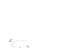
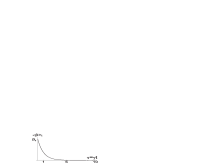
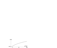
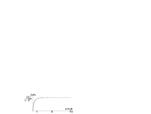
Figure 1: Figures on the left: evolution of the average of $\hat{x}$ and $\hat{p}$. Figures on the right: evolution of the variances ${\Delta x}_{t}$ and ${\Delta p}_{t}$. Parameter values (in SI units): $M=5.01\times 10^{-22},\quad m=5.01\times 10^{-26},\quad k_{B}=1.38\times 10^{-23},\quad\hbar=1.06\times 10^{-34},\quad\gamma=1000,\quad R=\gamma M/2m=5\times 10^{6},\quad T=300K,\quad p_{0}=5.01\times 10^{-26},\quad{\Delta x}_{0}=0.73\times 10^{-7},\quad{\Delta p}_{0}=7.26\times 10^{-28}\quad(\Delta_{\sigma}p)^{2}=(\Delta_{\sigma}x)^{2}=\frac{\hbar}{2}\times n,\quad n=10^{4}$. These parameters remain the same in all the following figures.

It is possible to calculate the evolution of the purity, $\mathrm{tr}(\hat{\rho}^{2})_{t}$, of the initial state of Eq. (17). This quantity, bounded by 0 and 1, is related to the linear entropy and is equal to 1 for pure states. Any difference from 1 means a loss of purity of the state. The purity of the Gaussian state is plotted in Fig. 2 as a function of time.

Figure 2: Behavior in time of $\mathrm{tr}(\hat{\rho}^{2})_{t}$.

The figure shows that the decoherence process occurs on a time scale much smaller than the relaxation time of the particle, which is of the order of $\gamma^{-1}$. The dynamics of our system are then described by the particle density matrix time evolution as a rapid transformation from the pure initial state (17) into a statistical mixture, as is shown in Fig. 3 in the coordinate representation.

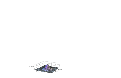
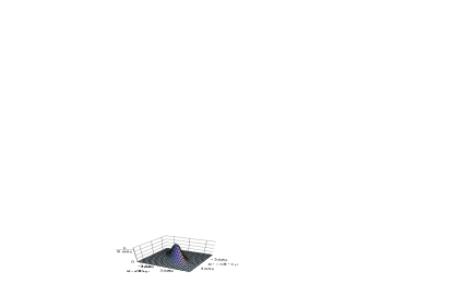
Figure 3: Left: Absolute value of the initial density matrix (17). Right: $|\rho(x,x^{\prime},t^{*})|$, where $t^{*}\ll\gamma^{-1}$. The suppression of the off-diagonal terms reflects the onset of decoherence before significant spreading has occurred.

To investigate further the dynamics of this loss of coherence both in $x$ and $p$ space we can compute the spreads $\mathcal{M}_{x}^{2}(t)$ and $\mathcal{M}_{p}^{2}(t)$, and coherence lengths, $\mathcal{L}_{x}(t)$ and $\mathcal{L}_{p}(t)$, using their general definition in [22] in terms of traces over the density matrix of the particle

$$\mathcal{M}_{x}^{2}(t)=\frac{\mathrm{Tr}(\hat{\rho}^{2}\hat{x}^{2})+\mathrm{Tr}(\hat{\rho}\hat{x}\hat{\rho}\hat{x})}{\mathrm{Tr}(\hat{\rho}^{2})}-2\left(\frac{\mathrm{Tr}(\hat{\rho}^{2}\hat{x})}{\mathrm{Tr}(\hat{\rho}^{2})}\right)^{2},$$ (24)

$$\mathcal{L}_{x}^{2}(t)=\frac{\mathrm{Tr}(\hat{\rho}^{2}\hat{x}^{2})-\mathrm{Tr}(\hat{\rho}\hat{x}\hat{\rho}\hat{x})}{\mathrm{Tr}(\hat{\rho}^{2})}\,,$$ (25)

with similar expressions for the momentum spread and coherence length. For pure states $\hat{\rho}^{2}=\hat{\rho}$ and therefore both spread and coherence length become equal to the respective width of the state, e.g. $\mathcal{M}_{x}(t)=\mathcal{L}_{x}(t)=\Delta x_{t}$. However, in presence of the interaction the state of the particle loses its initial purity and the two quantities differ. While $\mathcal{M}_{x}(t)$ gives the extension of the state, $\mathcal{L}_{x}(t)$ gives the zone inside the state extension, where coherence has not yet been lost at time $t$ [19].

For an initial Gaussian wave packet the spread $\mathcal{M}_{x}(t)$ corresponds to the width of the reduced density matrix along the main diagonal, $\mathcal{M}_{x}(t)=\Delta x_{t}=\int\rho(x,x,t)x^{2}-(\int\rho(x,x,t)x)^{2}$, while the coherence length $\mathcal{L}_{x}(t)$ gives analogously the width of the reduced density matrix along the main skew diagonal $\mathcal{L}_{x}(t)=\int\rho(x,-x,t)x^{2}-(\int\rho(x,-x,t)x)^{2}$.

The ratio $\mathcal{L}_{x}(t)/\mathcal{M}_{x}(t)$ gives a dimensionless measurement of the loss of coherence. It is interesting to note that for an initial Gaussian wave packet [23], this ratio is directly connected to $\mathrm{tr}(\hat{\rho}^{2})$ and is equal in both the position and momentum representations. This property is found also in our system where the following relations are obtained

$$\mathrm{tr}(\hat{\rho}^{2})_{t}=1-S_{lin}=\frac{\mathcal{L}_{x}(t)}{\Delta x_{t}}=\frac{\mathcal{L}_{p}(t)}{\Delta p_{t}}=\frac{\hbar/2}{\sqrt{4a_{t}c_{t}-b_{t}^{2}}}\,.$$ (26)

¿From Eqs. (26) and (20) we obtain

$$\mathcal{L}_{x}(t)\Delta p_{t}=\mathcal{L}_{p}(t)\Delta x_{t}=\frac{\hbar}{2}\sqrt{\frac{1}{1-b^{2}_{t}/4a_{t}c_{t}}}\geq\frac{\hbar}{2},$$ (27)

which can be seen as a particular case of the generalized uncertainty relation derived in [22].

The squares of the coherence lengths in the two representations are given by

$$\mathcal{L}_{x}^{2}(t)=\frac{\hbar^{2}a_{t}/2}{4a_{t}c_{t}-b_{t}^{2}}\quad\mathrm{and}\quad\mathcal{L}_{p}^{2}(t)=\frac{\hbar^{2}c_{t}/2}{4a_{t}c_{t}-b_{t}^{2}}\,.$$ (28)

It is instructive to consider the evolution of the coherence lengths at short times $(t\ll\gamma^{-1})$

$$\mathcal{L}_{x}^{2}(t)\approx\Delta x_{0}^{2}\left[1-2\left(\frac{D_{pp}}{\Delta p_{0}^{2}}-\gamma\right)t\right],\qquad\mathcal{L}_{p}^{2}(t)\approx\Delta p_{0}^{2}\left(1-2\frac{D_{xx}}{\Delta x_{0}^{2}}t\right)\,,$$ (29)

and for large times $(t\gg\gamma^{-1})$

$$\mathcal{L}_{x}^{2}(t)\approx\frac{\hbar^{2}}{4\Delta p_{t}^{2}}\approx\frac{\hbar^{2}\gamma}{4D_{pp}},\qquad\mathcal{L}_{p}^{2}(t)\approx\frac{\hbar^{2}}{4\Delta x_{t}^{2}}\,.$$ (30)

Eqs. (29) and (30) show the role of $D_{pp}$ and $D_{xx}$ in these evolutions, i.e. in the decoherence process. In particular, for small times the momentum coherence length $\mathcal{L}_{p}^{2}(t)$ depends only on the position diffusion $D_{xx}$, showing again the relevance of this term in this time region. This behaviour of $\mathcal{L}_{p}^{2}(t)$ can be understood by comparing it with that of $\mathcal{L}_{x}^{2}(t)$ which, as it is independent of $D_{xx}$, holds also in the Caldeira-Leggett model. Indeed, from Eqs. (29) and (22) we see that, as $\mathcal{L}_{x}^{2}(t)$ and $\Delta p^{2}_{t}$ both depend on the factor $\left(D_{pp}/\Delta p_{0}^{2}-\gamma\right)$, and the same occurs for $\mathcal{L}_{p}^{2}(t)$ and $\Delta x^{2}_{t}$, which both depend on $D_{xx}$.

3.2 Schrödinger cat state

The second configuration that we investigate is an initial Schrödinger cat state with a model wavefunction of the form

$$\psi(x,0)=\frac{1}{\sqrt{2\left[1+\exp\left(-\frac{l^{2}}{8\sigma^{2}}\right)\right]}(2\pi\sigma^{2})^{-\frac{1}{4}}}\times$$

$$\left\{\!\exp\!\left[\!-\frac{\left(x-\frac{l}{2}\right)^{2}}{4\sigma^{2}}-i\frac{Mv}{\hbar}x\right]\!+\!\exp\!\left[\!-\frac{\left(x+\frac{l}{2}\right)^{2}}{4\sigma^{2}}+i\frac{Mv}{\hbar}x\!\right]\!\right\}\ ,$$ (31)

where $\sigma$ is the width of two wave packets initially placed at a distance $l$ with one moving towards the other with an initial velocity $v$. Such states are interesting because of their potentially long-range coherence properties and the extreme sensitivity of this to environmental decoherence [24].

In the absence of any interactions the behaviour of the diagonal reduced density matrix elements is given by

$$\rho(x,x,t)=\frac{1}{2\left(1+\exp[-\frac{l^{2}}{8\sigma^{2}}]\right)\sqrt{2\pi\left(\sigma^{2}+\frac{\hbar^{2}t^{2}}{4M^{2}\sigma^{2}}\right)}}\left\{\exp\left[-\frac{(x-\frac{l}{2}+vt)^{2}}{2\left(\sigma^{2}+\frac{\hbar^{2}t^{2}}{4M^{2}\sigma^{2}}\right)}\right]+\right.$$

$$\left.\exp\left[-\frac{(x+\frac{l}{2}-vt)^{2}}{2\left(\sigma^{2}+\frac{\hbar^{2}t^{2}}{4M^{2}\sigma^{2}}\right)}\right]+\exp\left[-\frac{x^{2}+\left(\frac{l}{2}-vt\right)^{2}}{2\left(\sigma^{2}+\frac{\hbar^{2}t^{2}}{4M^{2}\sigma^{2}}\right)}\right]\cos\left[\frac{\frac{4Mv\sigma^{2}}{\hbar}+\frac{\hbar lt}{2\sigma^{2}M}}{2\left(\sigma^{2}+\frac{\hbar^{2}t^{2}}{4M^{2}\sigma^{2}}\right)}x\right]\right\}\,.$$ (32)

This probability distribution is the sum of three contributions. The first two clearly correspond to a pair of separately expanding (freely spreading) wave packets, while the third term represents an interference term, responsible for the central peak present in Fig. 4, which is a plot of Eq. (3.2). This is exactly as would be expected for such undamped evolution.

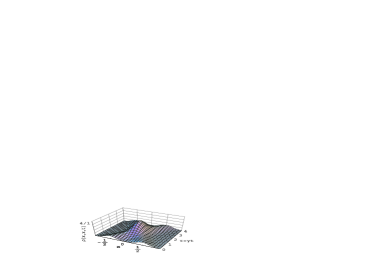
Figure 4: Free evolution of the diagonal reduced density matrix elements of Eq. (3.2). Used values (SI): $l=4\times 10^{-7},\sigma=0.73\times 10^{-7},v=10^{-4}$.

In B the time evolution is computed from the initial state of Eq. (3.2) using both the procedure described in Eq. (9) and the linearity of Eq. (7). Along the $x=x^{\prime}$ diagonal we find

$$\rho(x,x,t)=\frac{1}{2\left[1+\exp(-\frac{l^{2}}{8\sigma^{2}})\right]2\sqrt{\pi\bar{a}_{t}}}\left\{\exp\left[-\frac{(x+\bar{d}_{t})^{2}}{4\bar{a}_{t}}\right]+\exp\left[-\frac{(x-\bar{d}_{t})^{2}}{4\bar{a}_{t}}\right]\right.$$

$$\left.\!\!\!\!+\exp\!\left(-\frac{{x^{2}-|\bar{d}_{t}|}^{2}}{4\bar{a}_{t}}-\frac{2M^{2}v^{2}\sigma^{2}}{\hbar^{2}}-\frac{l^{2}}{8\sigma^{2}}\right)\cos\frac{|\bar{d}_{t}|x}{2\bar{a}_{t}}\right\},$$ (33)

with the evolution of the various coefficients given in Eq. (B). Eq. (3.2) reduces to Eq. (3.2) in the absence of any interaction, as may readily be verified by substituting $\lim_{\gamma\rightarrow 0}\Gamma/\gamma=t$ and $D_{pp}=D_{xx}=0$. This probability distribution is again the sum of three contributions. In order to investigate the behavior of the interference term, we compute the attenuation coefficient $W_{t}$ [25], defined as the ratio of the factor multiplying the cosine interference term to twice the geometric mean of the first two terms:

$$W_{t}=\exp\left[\frac{{\bar{d}_{t}}^{2}+|\tilde{d}_{t}|^{2}}{4a_{t}}-\frac{l^{2}}{8\sigma^{2}}-\frac{2M^{2}v^{2}\sigma^{2}}{\hbar^{2}}\right]\,.$$ (34)

In the free case $W_{t}=1$ for all times, corresponding to a full coherence. In the presence of interaction $W_{t}$ decays quickly, as pictured in Fig. 5, which shows the rapid destruction of the interference with time.

Figure 5: Evolution of the attenuation coefficient $W_{t}$.

By expanding $W_{t}$, for small times, in a Taylor series we find:

$$W_{t}\approx 1-D_{xx}\left(\frac{l^{2}}{4\sigma^{2}}+\frac{4M^{2}v^{2}\sigma^{2}}{\hbar^{2}}\right)t\,.$$ (35)

This equation shows that for very short times the attenuation factor decays with a characteristic time $\tau_{D}$ given by

$$\tau_{D}=\left[D_{xx}\left(\frac{l^{2}}{4\sigma^{2}}+\frac{4M^{2}v^{2}\sigma^{2}}{\hbar^{2}}\right)\right]^{-1}\,.$$ (36)

The interaction with the environment leads to the destruction of the interference term. The initial decay of $W_{t}$, which characterizes this, is due solely to the presence of the $D_{xx}$ term in Eq. (1). All of the decoherence occurs on a very short timescale and is due entirely to this diffusion.

In order to investigate further the dynamics of this loss of coherence in $x$ and $p$ space we compute the spreads, $\mathcal{M}_{x}^{2}(t)$ and $\mathcal{M}_{p}^{2}(t)$, and coherence lengths, $\mathcal{L}_{x}(t)$ and $\mathcal{L}_{p}(t)$ defined in Eqs. (24) and (25). By using Eq. (B) we obtain the spatial spread and the coherence length at time $t$

$$\mathcal{M}_{x}^{2}(t)=\frac{1}{8\bar{C}_{t}}+\frac{1}{8\bar{C}_{t}^{2}}\left\{\bar{E}_{t}^{2}\exp\left(\frac{\bar{E}_{t}^{2}}{2\bar{C}_{t}}-2\tilde{F}_{t}\right)-\tilde{E}_{t}^{2}\exp\left(-\frac{\tilde{E}_{t}^{2}}{2\bar{C}_{t}}-2\bar{F}_{t}\right)+\right.$$ (37)

$$\!\!\!\!\left.\left[\left(\bar{E}_{t}^{2}-\tilde{E}_{t}^{2}\right)\cos\alpha-2\bar{E}_{t}\tilde{E}_{t}\sin\alpha\right]\exp\left(-\beta\right)\rule{0.0pt}{14.22636pt}\right\}\div$$

$$\left\{\exp\left(\frac{\bar{E}_{t}^{2}}{2\bar{A}_{t}}-2\bar{F}_{t}\right)+\exp\left(\frac{\tilde{D}_{t}^{2}}{2\bar{A}_{t}}-2\tilde{F}_{t}\right)+\exp\left(-\frac{\bar{D}_{t}^{2}}{2\bar{A}_{t}}-2\bar{F}_{t}\right)+\exp\left(-\frac{\tilde{E}_{t}^{2}}{2\bar{A}_{t}}-2\tilde{F}_{t}\right)\right\}\,,$$

and

$$\mathcal{L}_{x}^{2}(t)=\frac{1}{8\bar{A}_{t}}+\frac{1}{8\bar{A}_{t}^{2}}\left\{\tilde{D}_{t}^{2}\exp\left(\frac{\tilde{D}_{t}^{2}}{2\bar{A}_{t}}-2\tilde{F}_{t}\right)-{\bar{D}_{t}}^{2}\exp\left(-\frac{{\bar{D}_{t}}^{2}}{2\bar{A}_{t}}-2\bar{F}_{t}\right)+\right.$$

$$\left.\left[\left(\tilde{D}_{t}^{2}-\bar{D}_{t}^{2}\right)\cos\alpha-2\bar{D}_{t}\tilde{D}_{t}\sin\alpha\right]\exp\left(-\beta\right)\rule{0.0pt}{14.22636pt}\right\}\div$$

$$\left\{\exp\left(\frac{\bar{E}_{t}^{2}}{2\bar{A}_{t}}-2\bar{F}_{t}\right)+\exp\left(\frac{\tilde{D}_{t}^{2}}{2\bar{A}_{t}}-2\tilde{F}_{t}\right)+\exp\left(-\frac{\bar{D}_{t}^{2}}{2\bar{A}_{t}}-2\bar{F}_{t}\right)+\exp\left(-\frac{\tilde{E}_{t}^{2}}{2\bar{A}_{t}}-2\tilde{F}_{t}\right)\right\}\,,$$

where $\alpha=\left(\bar{C}_{t}\bar{D}_{t}\tilde{D}_{t}+\bar{A}_{t}\bar{E}_{t}\tilde{E}_{t}\right)/4\bar{A}_{t}\bar{C}_{t}+\bar{F}_{t}+\tilde{F}_{t}$ and $\beta=\left[\bar{C}_{t}\bar{D}_{t}^{2}-\bar{C}_{t}\tilde{D}_{t}^{2}+A\tilde{E}_{t}^{2}-\bar{A}_{t}\bar{E}_{t}^{2}\right]$ $/8\bar{A}_{t}\bar{C}_{t}$. In order to obtain the same quantities in momentum space we need the corresponding reduced density matrix. If we perform a double Fourier transform we obtain $\rho(p,p^{\prime},t)$ from $\rho(x,x^{\prime},t)$. The result has the same form as Eq. (B) with the following substitutions:

$$\bar{A}_{t}\!\!\rightarrow\!\!\frac{\bar{A}_{t}}{Z_{t}},\quad\bar{B}_{t}\rightarrow\frac{-\bar{B}_{t}}{\bar{Z}_{t}},\quad\bar{C}_{t}\rightarrow\frac{\bar{C}_{t}}{Z_{t}},\quad\bar{D}_{t}\!\!\rightarrow\!\!2\hbar\frac{\bar{B}_{t}\bar{D}_{t}+2\bar{A}_{t}\bar{E}_{t}}{Z_{t}},\quad\tilde{D}_{t}\rightarrow-2\hbar\frac{\bar{B}_{t}\tilde{D}_{t}+2\bar{A}_{t}\tilde{E}_{t}}{Z_{t}},$$

$$\bar{E}_{t}\!\!\rightarrow\!\!2\hbar\frac{\bar{B}_{t}\bar{E}_{t}-2\bar{C}_{t}\bar{D}_{t}}{Z_{t}},\quad\tilde{E}_{t}\rightarrow 2\hbar\frac{\bar{B}_{t}\tilde{E}_{t}-2\bar{C}_{t}\tilde{D}_{t}}{Z_{t}},\quad\bar{F}_{t}\!\!\rightarrow\!\!\bar{F}_{t}\!\!+\frac{\ln\!Z_{t}}{2}+$$

$$4\hbar^{2}\frac{\bar{C}_{t}\bar{D}_{t}^{2}-\bar{B}_{t}\bar{D}_{t}\bar{E}_{t}-\bar{A}_{t}\bar{E}_{t}^{2}}{Z_{t}},\quad\tilde{F}_{t}\!\!\rightarrow\!\!\tilde{F}_{t}\!\!+\frac{\ln\!Z_{t}}{2}+4\hbar^{2}\frac{\bar{C}_{t}\tilde{D}_{t}^{2}-\bar{B}_{t}\tilde{D}_{t}\tilde{E}_{t}-\bar{A}_{t}\tilde{E}_{t}^{2}}{Z_{t}},$$ (39)

where $Z_{t}=4(\bar{B}_{t}^{2}+4\bar{A}_{t}\bar{C}_{t})\hbar^{2}$. By using these substitutions in Eqs. (37) and (3.2) one obtains the corresponding $\mathcal{M}_{p}^{2}(t)$ and $\mathcal{L}_{p}^{2}(t)$.

These quantities satisfy $\mathcal{M}_{x}(0)=\mathcal{L}_{x}(0)$ and $\mathcal{M}_{p}(0)=\mathcal{L}_{p}(0)$ at the initial time, while for large times their increase is the same as the corresponding quantities $\Delta x_{t}$, $l_{x}(t)$, $\Delta p_{t}$ and $l_{p}(t)$ in Eqs. ( 23) and (30) found for the single Gaussian wave packet. In particular it has been shown that a generalized uncertainty relation holds [22]

$$\mathcal{L}_{x}(t)\mathcal{M}_{p}(t)\geq\frac{\hbar}{2}\,.$$ (40)

This product is plotted in Fig. 6 for our cat state, which shows how the uncertainty relation is satisfied at all times.

Figure 6: The evolution of the product $\mathcal{L}_{x}(t)\mathcal{M}_{p}(t)$.

4 Unphysical parameter region

As was stated in the introduction, one of the key differences between Eq. (1) and the Caldeira Leggett equation is the presence of the $D_{xx}$ term. The latter master equation, of course, is not of the Lindblad type and pathological behavior has been observed by several authors [19, 13, 18] if $\gamma$ is too large or the wave packet width too small (smaller than the thermal de Broglie wavelength of the object). If we consider the time derivative of the linear entropy for small times, then we would expect a positive value for an initial pure state, for which $S_{lin}=0$. In our model we find this time derivative to be

$$\frac{\mathrm{d}}{\mathrm{d}t}S_{lin}|_{t=0}=-\frac{\mathrm{d}}{\mathrm{d}t}\mathrm{tr}\hat{\rho}^{2}|_{t=0}=-2\langle\dot{\hat{\rho}}\rangle=\frac{4}{\hbar^{2}}{{\Delta p}_{0}}^{2}D_{xx}+\frac{4}{\hbar^{2}}{{\Delta x}_{0}}^{2}D_{pp}-\gamma\,,$$ (41)

where the brackets indicate the average over a general state of the Brownian particle and we have used Eq. (1) to obtain the last equality. If we use ${\Delta x}_{0}{\Delta p}_{0}=\frac{\hbar}{2}$, then the positivity of Eq. (41) is assured for all possible states only if

$$D_{xx}D_{pp}\geq\left(\frac{\hbar\gamma}{4}\right)^{2}\,.$$ (42)

This is the same condition as that found in [13] by requiring an initial reduction in the probability of remaining in the initial pure state.

Even if in our model this condition is satisfied by our parameters of Eqs. (3) and (4) it is interesting to work near the region of its validity. In fact we can use our master equation Eq. (1), and look for anomalous features when Eq. (42) is not satisfied. For example, after substituting $D_{pp}=q\frac{\left(\hbar\gamma/4\right)^{2}}{D_{xx}}$, we can vary $q$ around one. In Fig. 7 Eq. (41) is plotted as a function of $q$.

Figure 7: Behavior of the derivative of the linear entropy at $t=0$ as a function of $q$.

This figure clearly shows that the rate of change of linear entropy is negative at small times if the Lindblad condition is not satisfied.

5 Conclusions and discussion

In this paper we have used the Lindblad master equation for Brownian motion found in [12, 13] to analyze wave packet dynamics. To this end we have provided a simple and clear scheme by which we can obtain the exact time evolution starting from general initial conditions.

We have applied this procedure to find the time evolution of two initial states: the first in which the Brownian particle is represented by a Gaussian wave packet and the second, in which it is represented by a Schrödinger cat state. In each case we have provided expressions for the relevant quantities in both the position and momentum representations. There are complementary aspects of the two representations, such as generalized uncertainty relations not found when one focuses only on the spatial features.

We have analyzed further the dissipation and decoherence, in particular focusing on the reduced density matrix evolution in the coordinate representation. We have obtained the evolution of the wavepacket widths and the coherence lengths for both initial conditions and in both the position and momentum representations. The Gaussian wave packet shows a very rapid decoherence on a timescale much shorter than the relaxation time of the system. In the momentum representation this decoherence depends only on the position diffusion coefficient, $D_{xx}$, present in the master equation. The $D_{xx}$ term is also the only term responsible for the increase in the spatial width of the wave packet for small times. The term containing this coefficient is absent in many previous master equations which have been used to describe friction and Brownian motion.

The evolution of a Schrödinger cat state without any frictional effects shows coherent oscillations caused by interference between the two components of the wave function. Our analysis shows that such interference is damped on timescales again much shorter than the relaxation time; decoherence is very rapid. We have quantified the decoherence using an attenuation coefficient for the oscillatory terms. This attenuation coefficient also depends on $D_{xx}$. The results of the computation of generalized variances and coherence lengths show that for large times these quantities behave in a similar way to the single Gaussian wave packet case, and that a generalized uncertainty relation between variances and coherence lengths holds for all times.

Finally we have generalized the system to look at the case where the product of the diffusion coefficients is not large enough to guarantee that the master equation is of Lindblad form. Here we see a clear signature of unphysical behaviour in the linear entropy, which is associated with probabilities outside the physically-meaningful range between 0 and 1.

The measurement-based quantum description of friction illustrated in this paper provides a general framework for investigating the role that the various terms in the master equation play in decoherence. It is clear from our analysis that the two extra diffusion terms not associated with the temperature of the system are necessary to ensure complete positivity of the density operator at all times. This is consistent with previous work [12, 13]. The minimum sizes of these terms are governed by an uncertainty relation, in line with their wholly quantum origin. Diffusion in one observable is associated with localization in the complementary one. These localizations occur each time a measurement is made. The consequent diffusion, and in particular that of position, which has no analogue in the Caldeira-Leggett reservoir-based approach, must be taken account of in any complete quantum description of friction. The cost of not doing so is illustrated emphatically here; the resultant incomplete equation cannot describe decoherence correctly, because it is not valid on the short timescales during which decoherence occurs.

The generality of the measurement-based approach reflects the generality of the Kraus formalism of quantum measurements on which it is based, which makes no reference to any particular measurement device. Consequently the theory presented here is not specific to any particular frictional or Brownian system. Such a linkage could in principle be found for particular systems, and would amount to an ab initio quantum theory of friction. No such theory is known at this time.

Appendix A

In this appendix we use the method of characteristics [21] to solve the master equation of Eq. (7). The first step is to rewrite Eq. (7) as

$$1\frac{\partial\rho(k,\Delta_{t},t)}{\partial t}+\left(\gamma\Delta_{t}-\frac{k}{M}\right)\frac{\partial\rho(k,\Delta_{t},t)}{\partial\Delta_{t}}=-\left(D_{pp}\Delta_{t}^{2}+D_{xx}k^{2}\right)\rho(k,\Delta_{t},t)\,.$$ (43)

The curves in the $t,\Delta_{t}$ plane, parameterized by $l$ and defined by the relation

$$\frac{\mathrm{d}t}{1}=\frac{\mathrm{d}\Delta_{t}}{\gamma\Delta_{t}-\frac{k}{M}}=\mathrm{d}l\,,$$ (44)

are called the characteristic curves of the partial differential equations. Eq. (44) may be written as:

$$\frac{\mathrm{d}t}{1}=\frac{\mathrm{d}\Delta_{t}}{\gamma\Delta_{t}-\frac{k}{M}}=-\frac{\mathrm{d}\rho(k,\Delta_{t},t)}{\left(D_{pp}\Delta^{2}_{t}+D_{xx}k^{2}\right)\rho(k,\Delta_{t},t)}\,.$$ (45)

This pair of equations, valid on each characteristic curve, enables a general solution of the partial differential equation (43) to be found as follows. We perform a first integration using the first equality of Eq. (45), finding for one arbitrary constant $W$:

$$W=\mathrm{e}^{-\gamma t}\left({\Delta_{t}-\frac{k}{\gamma M}}\right)\,,$$ (46)

from which it follows at $t=0$

$$W={\Delta_{0}-\frac{k}{\gamma M}}\,,$$ (47)

as $k$ is independent of time. Now we perform a second integration using the second equality in Eq. (45), finding a second arbitrary constant $Z$:

$$Z=\frac{1}{\rho(k,\Delta_{t},t)}\exp\left[-\frac{D_{pp}\Delta_{t}^{2}}{2\gamma}-\frac{D_{pp}k\Delta_{t}}{M\gamma^{2}}\right]\left({\Delta_{t}-\frac{k}{\gamma M}}\right)^{-\frac{k^{2}}{\gamma}\big{(}D_{xx}+\frac{D_{pp}}{M^{2}\gamma^{2}}\big{)}}\,,$$ (48)

from which it follows at $t=0$

$$Z=\frac{1}{\rho(k,\Delta_{0},0)}\exp\left[-\frac{D_{pp}\Delta_{0}^{2}}{2\gamma}-\frac{D_{pp}k\Delta_{0}}{M\gamma^{2}}\right]\left({\Delta_{0}-\frac{k}{\gamma M}}\right)^{-\frac{k^{2}}{\gamma}\big{(}D_{xx}+\frac{D_{pp}}{M^{2}\gamma^{2}}\big{)}}\,.$$ (49)

By using Eq. (49) in Eq. (48) we find for $\rho(k,\Delta_{t},t)$:

$$\!\!\!\!\rho(k,\Delta_{t},t)= \rho(k,\Delta_{0},0)\exp\left[-\frac{D_{pp}\left(\Delta_{t}^{2}-\Delta_{0}^{2}\right)}{2\gamma}-\frac{D_{pp}k\left(\Delta_{t}-\Delta_{0}\right)}{M\gamma^{2}}\right]$$ (50)

$$\times\left(\frac{{\Delta_{t}-\frac{k}{\gamma M}}}{{\Delta_{0}-\frac{k}{\gamma M}}}\right)^{-\frac{k^{2}}{\gamma}\big{(}D_{xx}+\frac{D_{pp}}{M^{2}\gamma^{2}}\big{)}}\,.$$

In order to express $\Delta_{t}$ as a function of $\Delta_{0}$ we use Eqs. (46) and (47), finding

$$\Delta_{0}=\Delta_{t}\mathrm{e}^{-\gamma t}+\frac{k}{\gamma M}\left(1-\mathrm{e}^{-\gamma t}\right)\,.$$ (51)

Substituting the previous expression for $\Delta_{0}$ in Eq. (50), we finally obtain for $\rho(k,\Delta_{t},t)$:

$$\rho(k,\Delta_{t},t)=\rho\left(k,\Delta_{t}(1-\Gamma)+\frac{k}{\gamma M}\Gamma,0\right)\times$$ (52)

$$\exp\left\{\left[-\left(D_{xx}+\frac{D_{pp}}{M^{2}\gamma^{2}}\right)t+\frac{D_{pp}}{M^{2}\gamma^{3}}\left(\frac{\gamma^{2}}{2}+\Gamma\right)\right]k^{2}-\frac{D_{pp}\gamma^{2}}{M\gamma^{2}}k\Delta_{t}-\frac{D_{pp}\Gamma(2-\Gamma)}{2\gamma}\Delta^{2}_{t}\,\right\}\,,$$

where $\Gamma=1-\exp(-\gamma t)$.

Appendix B

In this appendix we obtain the time evolution of the Schrödinger cat initial state given in Eq. (3.2).

Computing the reduced density matrix $\rho(x,x^{\prime},0)$ corresponding to Eq. (3.2) and using Eq. (6) to move to the $(k,\Delta_{t})$ representation we obtain:

$$\rho(k,\Delta_{0},0)=\frac{1}{2\left(1+\exp[-\frac{l^{2}}{8\sigma^{2}}]\right)}\left\{\exp\left[-\frac{\sigma^{2}}{2}k^{2}-\frac{\hbar^{2}}{8\sigma^{2}}\Delta_{0}^{2}+i\frac{l}{2}k-iMv\Delta_{0}\right]+\right.$$

$$\left.\exp\!\left[-\frac{\sigma^{2}}{2}k^{2}-\frac{\hbar^{2}}{8\sigma^{2}}\Delta_{0}^{2}-i\frac{l}{2}k+Mv\Delta_{0}\right]\!+\!\left(\exp\!\left[-\frac{\sigma^{2}}{2}k^{2}-\frac{\hbar^{2}}{8\sigma^{2}}\Delta_{0}^{2}-\frac{2Mv\sigma^{2}}{\hbar}k-\frac{\hbar l}{4\sigma^{2}}\Delta_{0}\right]\right.\right.$$

$$\left.\left.+\exp\left[-\frac{\sigma^{2}}{2}k^{2}-\frac{\hbar^{2}}{8\sigma^{2}}\Delta_{0}^{2}+\frac{2Mv\sigma^{2}}{\hbar}k+\frac{\hbar l}{4\sigma^{2}}\Delta_{0}\right]\right)\times\exp\left[-\frac{2M^{2}v^{2}\sigma^{2}}{\hbar^{2}}-\frac{l^{2}}{8\sigma^{2}}\right]\right\}\,.$$ (53)

The form of this initial condition is of the kind:

$$\rho(k,\Delta_{0},0)=\sum_{j=1}^{4}\rho_{j}(k,\Delta_{0},0)\,,$$ (54)

where comparing with Eq. (11) we have for the various coefficients the initial values

$$a^{1,2,3,4}_{0}=\frac{\sigma^{2}}{2},\quad b^{1,2,3,4}_{0}=0,\quad c^{1,2,3,4}_{0}=\frac{\hbar^{2}}{8\sigma^{2}},\quad d^{1}_{0}=-d^{2}_{0}=-\frac{l}{2},\quad d^{3}_{0}=-d^{4}_{0}=-i\frac{2Mv\sigma^{2}}{\hbar},$$

$$e^{1}_{0}=-e^{2}_{0}=Mv,\quad e^{3}_{0}=-e^{4}_{0}=-i\frac{\hbar d}{4\sigma^{2}},\quad f^{1,2}_{0}=\ln 2\left[1-\exp\left(-\frac{d^{2}}{8\sigma^{2}}\right)\right],$$

$$f^{3,4}_{0}=\ln 2\left(1-\exp\left[-\frac{d^{2}}{8\sigma^{2}}\right]\right)+\frac{2M^{2}v^{2}\sigma^{2}}{\hbar^{2}}+\frac{l^{2}}{8\sigma^{2}}\,.$$ (55)

By using Eq. (2) it is possible to compute the time evolution of all the coefficients of the four parts of Eq. (54):

$$a^{1,2,3,4}_{t}=\bar{a}_{t}=\frac{\sigma^{2}}{2}+\frac{\hbar^{2}}{8\sigma^{2}}\frac{\gamma^{2}}{M^{2}\gamma^{2}}+\left(D_{xx}+\frac{D_{pp}}{M^{2}\gamma^{2}}\right)t-\frac{D_{pp}}{M^{2}\gamma^{3}}\left(\frac{\Gamma^{2}}{2}+\Gamma\right),$$

$$b^{1,2,3,4}_{t}=\bar{b}_{t}=\frac{\hbar^{2}}{8\sigma^{2}}\frac{2\Gamma(1-\Gamma)}{M\gamma}+\frac{D_{pp}\Gamma^{2}}{M\gamma^{2}},\quad c^{1,2,3,4}_{t}=\bar{c}_{t}=\frac{\hbar^{2}}{8\sigma^{2}}(1-\Gamma)^{2}+\frac{D_{pp}\Gamma(2-\Gamma)}{2\gamma},$$

$$d^{1}_{t}=-d^{2}_{t}=\bar{d}_{t}=-\frac{l}{2}+\frac{v\Gamma}{\gamma},\quad d^{3}_{t}=-d^{4}_{t}=\tilde{d}_{t}=-i\left(\frac{2Mv\sigma^{2}}{\hbar}+\frac{\hbar l}{4\sigma^{2}}\frac{\Gamma}{M\gamma}\right),$$

$$e^{1}_{t}=-e^{2}_{t}=\bar{e}_{t}=Mv(1-\Gamma),\quad e^{3}_{t}=-e^{4}_{t}=\tilde{e}_{t}=-i\frac{\hbar l}{4\sigma^{2}}(1-\Gamma),$$

$$f^{1,2}_{t}=f^{1,2}_{0}=\bar{f}_{t},\quad f^{3,4}_{t}=f^{3,4}_{0}=\tilde{f}_{t}\,.$$ (56)

Then using Eq. (15) we can move to coordinate representation obtaining for the reduced density matrix

$$\rho(x,x^{\prime},t)=\sum_{j=1}^{4}\rho_{j}(x,x^{\prime},t)=\sum_{j=1}^{4}\exp\!\left[-A^{j}_{t}(x-x^{\prime})^{2}-iB^{j}_{t}(x-x^{\prime})(x+x^{\prime})-\right.$$

$$\left.C^{j}_{t}(x+x^{\prime})^{2}-iD^{j}_{t}(x-x^{\prime})-E^{j}_{t}(x+x^{\prime})-F^{j}_{t}\right],$$ (57)

where

$$A^{1,2,3,4}_{t}=\bar{A}_{t}=\frac{4\bar{a}_{t}\bar{c}_{t}-\bar{b}_{t}^{2}}{4\hbar^{2}\bar{a}_{t}},\quad B^{1,2,3,4}_{t}=\bar{B}_{t}=-\frac{\bar{b}_{t}}{4\hbar\bar{a}_{t}},\quad C^{1,2,3,4}_{t}=\bar{C}_{t}=\frac{1}{16\bar{a}_{t}},$$

$$D^{1}_{t}=-D^{2}_{t}=\bar{D}_{t}=\frac{2\bar{a}_{t}\bar{e}_{t}-\bar{b}_{t}\bar{d}_{t}}{2\hbar\bar{a}_{t}},\quad D^{3}_{t}\!=\!-D4_{t}\!=\!\frac{2\bar{a}_{t}\tilde{e}_{t}-\bar{b}_{t}\tilde{d}_{t}}{2\hbar\bar{a}_{t}}\!=\!\tilde{D}_{t},\,\,\,E^{1}_{t}=-E^{2}_{t}=\bar{E}_{t}=\frac{\bar{d}_{t}}{4\bar{a}_{t}},$$

$$E^{3}_{t}=-E^{4}_{t}=\tilde{E}_{t}=\frac{\tilde{d}_{t}}{4\bar{a}_{t}},\quad\exp(-F^{1,2}_{t})=\exp(-\bar{F}_{t})=\frac{\exp(-\bar{f}_{t})}{2\sqrt{\pi\bar{a}_{t}}}\exp\!\!\left[-\frac{\bar{d}_{t}^{2}}{4\bar{a}_{t}}\right],$$

$$\exp(-F^{3,4}_{t})=\exp(-\tilde{F}_{t})=\frac{\exp(-\tilde{f}_{t})}{2\sqrt{\pi\bar{a}_{t}}}\exp\!\!\left[-\frac{\tilde{d}_{t}^{2}}{4\bar{a}_{t}}\right].$$ (58)

Next from the last equation in Eq. (B) it follows that

$$\rho(x,x^{\prime},t)=\exp\!\!\left[-\bar{A}_{t}(x-x^{\prime})^{2}\!-i\bar{B}_{t}(x-x^{\prime})(x+x^{\prime})\!-\bar{C}_{t}(x+x^{\prime})^{2}\right]\times$$

$$\left\{\exp\!\!\left[-i\bar{D}_{t}(x-x^{\prime})-\bar{E}_{t}(x+x^{\prime})-\bar{F}_{t}\right]\exp\!\!\left[+i\bar{D}_{t}(x-x^{\prime})+\bar{E}_{t}(x+x^{\prime})-\bar{F}_{t}\right]\right.$$

$$+\left.\exp\!\!\left[-i\tilde{D}_{t}(x-x^{\prime})-\tilde{E}_{t}(x+x^{\prime})-\tilde{F}_{t}\right]+\exp\!\!\left[+i\tilde{D}_{t}(x-x^{\prime})+\tilde{E}_{t}(x+x^{\prime})-\tilde{F}_{t}\right]\right\}\,.$$ (59)

Along the diagonal we have

$$\rho(x,x,t)=\frac{1}{2\left[1+\exp(-\frac{l^{2}}{8\sigma^{2}})\right]2\sqrt{\pi\bar{a}_{t}}}\left\{\exp\left[-\frac{(x+\bar{d}_{t})^{2}}{4\bar{a}_{t}}\right]+\exp\left[-\frac{(x-\bar{d}_{t})^{2}}{4\bar{a}_{t}}\right]\right.$$

$$\left.\!\!\!\!+\exp\!\left(-\frac{{x^{2}-|\bar{d}_{t}|}^{2}}{4\bar{a}_{t}}-\frac{2M^{2}v^{2}\sigma^{2}}{\hbar^{2}}-\frac{l^{2}}{8\sigma^{2}}\right)\cos\frac{|\bar{d}_{t}|x}{2\bar{a}_{t}}\right\}.$$ (60)

References

- [1] Caldeira A O and Leggett A J 1983 Physica 121A 587
- [2] Hu B L, Paz J P and Zhang Y 1992 Phys. Rev.D 45 2843
- [3] Sandulescu A and Scutaru 1987 Ann. Phys., NY173 277
- [4] Gallis M R 1993 Phys. Rev.A 48 1028
- [5] Joos E and Zeh H D 1985 Z. Phys.Ann. Phys. B: Condens. Matter 59 223
- [6] Diòsi L 1995 Europhys. Lett. 30 63
- [7] Horneberger K and Sipe J E 2003 Phys. Rev.A 68 012105
- [8] Scott A J and Milburn G J 2001 Phys. Rev.A 63 042101
- [9] Mensky M B and Stenholm S 2003 Phys. Lett.A 308 243
- [10] Breuer H P and Petruccione F 2002 The Theory of Open Quantum Systems (Oxford University)
- [11] Zwanzig R 1973 J. Stat. Phys. 9 215
- [12] Barnett S M and Cresser J D 2005 Phys. Rev.A 72 022107
- [13] Barnett S M, Jeffers J and Cresser J D 2006 J. Phys.: Condens. Matter 18 S401
- [14] Lindblad G 1976 Commun. Math. Phys. 48 119
- [15] Cresser J D, Barnett S M, Jeffers J and Pegg D T 2006 Opt. Commun. 264, 352
- [16] Busch P, Grabowski M and Lahti P 1995 Operational Quantum Physics (Springer-Verlag, Berlin)
- [17] Ambegaokar V. 1991 Ber. Bunsenges. Phys. Chem. 95 400
- [18] Stenholm S 1994 in Quantum Dynamics of Simple Systems, Proceedings of the 44th Scottish Universities Summer School in Physics, edited by Oppo G -L, Barnett S M, Riis E and Wilkinson M (IOP Publishing, Bristol)
- [19] Joos E, Zeh H D, Kiefer C, Giulini D, Kupsch J and Stamatescu I O 2002 Decoherence and the Appearance of a Classical World in Quantum Theory (Springer, New York, sec. ed.)
- [20] Unruh W G and Zurek W H 1989 Phys. Rev.D 40 1071
- [21] Barnett S M and Radmore P M 1997 Methods in Theoretical Quantum Optics (Oxford University Press, New York).
- [22] Franke-Arnold S, Huyet G and Barnett S M 2001 J. Phys. B 34 945
- [23] Morikawa M 1990 Phys. Rev.D 42 2929
- [24] Brune M, Hagley E, Dreyer J, Ma tre X, Maali A, Wunderlich C, Raimond J M, and Haroche S 1996 Phys. Rev. Lett.77 4887
- [25] Ford G W and O’Connell R F 2001 Phys. Lett.A 286 87