KA-TP-16-2007

Black-Body Anomaly: Analysis of Temperature Offsets

Michal Szopa^∗∗, Ralf Hofmann^∗, Francesco Giacosa^†, and
Markus Schwarz^∗

$\mbox{}^{**}$ Institut für Theoretische Physik
Universität Heidelberg
Philosophenweg 16
69120 Heideberg, Germany

$\mbox{}^{*}$ Institut für Theoretische Physik
Universität Karlsruhe
Kaiserstr. 12
76131 Karlsruhe, Germany

$\mbox{}^{\dagger}$ Institut für Theoretische Physik
Universität Frankfurt
Johann Wolfgang Goethe - Universität
Max von Laue–Str. 1
60438 Frankfurt, Germany

Based on the postulate that photon propagation is governed by a dynamically broken SU(2) gauge symmetry (scale $\sim 10^{-4}\,$eV) we make predictions for temperature offsets due to a low-temperature (a few times the present CMB temperature) spectral anomaly at low frequencies. Temperature offsets are extracted from least-square fits of the anomalous black-body spectra to their conventional counterparts. We discuss statistical errors, compare our results with those obtained from calibration data of the FIRAS instrument, and point out that our predicted offsets are screened by experimental errors given the frequency range used by FIRAS to perform their spectral fits. We also make contact with the WMAP observation by blueshifting their frequency bands. Although our results hint towards a strong dynamical component in the CMB dipole and an explanation of low-$l$ suppression it is important in view of its particle-physics implications that the above postulate be verified/falsified by an independent low-temperature black-body precision experiment.

1 Introduction

The existence of the cosmic microwave background (CMB) was theoretically predicted a long time ago [1]. Its definite discovery, which gives tremendous support to the Hot Big Bang model, was announced almost twenty years later [2]. An important result of the Cosmic Background Explorer (COBE) mission and in particular its Far-Infrared Absolute Spectrometer (FIRAS) was the observation of a black-body spectral shape of the CMB radiation in the frequency range from 1 or 2 cm^-1 to 20 cm^-1 with temperature uncertainties of at most a few milli Kelvin [3, 4, 5, 6].

A successor satellite experiment, the Wilkinson Microwave Anisotropy Probe (WMAP) [7, 8], recorded the full-sky maps of temperature variations by observing this near-to-perfect black-body spectrum within five fixed frequency bands, $\nu=23,33,41,61,$ and 94 GHz, picked in such a way as to minimize the contamination of the CMB signal by the galactic and the solar-system foregrounds.

Based on the postulate that photon propagation is described by an SU(2) Yang-Mills theory [9, 10] a spectral black-body (BB) anomaly was predicted to occur in the low-temperature, low-frequency realm [11, 12]. Namely, for frequencies below a temperature-dependent critical value the BB spectral intensity vanishes because of photon screening. Above this critical frequency there is a small range of antiscreening. Both effects are due to the nonabelian nature of the theory, see [12] and Sec. 2. Because of its association with the CMB, whose present temperature determines the Yang-Mills scale to $\Lambda\sim 10^{-4}\,$eV$\sim T_{\tiny\mbox{CMB}}=2.73$ K, the name SU(2)${}_{\tiny\mbox{CMB}}$ was introduced.

The thermodynamics of an SU(2) (or SU(3)) Yang-Mills theory is approached by addressing the (microscopically highly complex) dynamics of the ground state in terms of an effective theory obtained by coarse-graining the topologically nontrivial sector [13]. SU(2) Yang-Mills thermodynamics comes in three phases: A deconfining one for temperatures $T\geq T_{c}\sim\Lambda$, a preconfining one for $T\sim\Lambda$, and a confining one for $T<\Lambda$, for more detail see Sec. 2.

As for the modification of the radiation law of a black body by nonabelian effects the deconfining phase of SU(2)${}_{\tiny\mbox{CMB}}$ is relevant. For an analysis of the viability of SU(2)${}_{\tiny\mbox{CMB}}$ see [14]. Other interesting predictions, such as the duration of the present cosmological epoch of supercooling [14], require quantitative knowledge about the preconfining phase. In that phase the photon nonperturbatively acquires a (Meissner) mass.

In connection with the onset of a superconducting ground state let us consider a photon gas contained in a small spatial region immersed in the CMB, a satellite for example. When cooling this gas below $T_{\tiny{\mbox{CMB}}}$ the associated ground state would be preconfining (massive photon) if it were not for the large-range correlation in the surrounding CMB ground state which prevents this transition from occurring (supercooled situation). The physical effect associated with tunneling transitions between the two ground states is an increase of the effective number of photon polarizations. The effect depends on the ratio between correlation length and linear dimension of the cold-spot volume. For details see Sec. 3.2.2 below.

The occurrence of a BB anomaly for $T>T_{\tiny\mbox{CMB}}$ and low frequencies has a profound impact on the CMB temperature-temperature correlations at large angles. The suppression of the latter after subtracting the CMB monopole and dipole and the violation of statistical isotropy at low $l$ [15] is likely to be understood by this anomaly. In [16] a dynamically generated component to the CMB dipole was considered to be due to the BB anomaly.

The purpose of the present paper is an analysis of the present experimental/observational situation concerning the afore-mentioned BB anomaly. We concentrate on two satellite-based experiments. First, we explore the consequences of the BB anomaly for offsets between the known wall temperature and the fitted temperature of radiation when assuming the latter to be spectrally distributed according to Planck’s law. This was the strategy used in the temperature calibration stage of FIRAS. The calibration was performed both on Earth and in orbit with differing results. Here we would like to compare our theoretical results with their in-flight data. Apart from an interesting signature at $T<T_{\tiny\mbox{CMB}}$ and a large negative (global) offset for $T>T_{\tiny\mbox{CMB}}$, which we discuss in view of SU(2)${}_{\tiny\mbox{CMB}}$, we conclude that for fits within the above-quoted FIRAS frequency range the effect of the theoretically predicted BB anomaly is too small to rise above the experimental errors.

Second, we would like to make contact with the WMAP satellite (temperature fits within the above-quoted but blueshifted frequency bands). Since blueshifted spectra are related to the angular resolution in the temperature-temperature correlation function we are in a position to semi-quantitatively compare observationally determined temperature offset for $T>T_{\tiny\mbox{CMB}}$ with theory.

The article is organized as follows. For the benefit of the reader, we quote a number of essential results for deconfining SU(2) Yang-Mills thermodynamics in Sec. 2. In Sec. 3 we first describe the relevant results for temperature offsets in the low-temperature realm as measured and observed by FIRAS and WMAP, respectively. Within the setting of FIRAS we then perform spectral fits to theoretical predictions based on SU(2)${}_{\tiny\mbox{CMB}}$, and we discuss our results. As a next step, we perform an analogous program for the blueshifted WMAP frequency bands and discuss these results in view of the low TT multipoles in the CMB. Finally, we extract temperature offsets from integrated spectra and point out the difference compared with spectral fits. In Sec. 4 we summarize our results and conclude.

2 Effective SU(2) Yang-Mills thermodynamics

In this section we briefly describe the effective theory for SU(2) Yang-Mills thermodynamics. The basic ingredient is an adjoint scalar field $\phi$, which represents (part of) the thermal ground state emerging from a spatial average over interacting calorons and anticalorons of topological charge modulus $|Q|=1$. The scalar field $\phi$ is an inert background field to the dynamics of topologically trivial, coarse-grained gauge fields $a_{\mu}$ entering in the effective field strength $G_{\mu\nu}^{a}=\partial_{\mu}(a_{\nu}^{a})-\partial_{\nu}(a_{\mu}^{a})-e\varepsilon^{abc}a_{\mu}^{b}a_{\nu}^{c}$. The temperature dependent effective coupling $e=e(T)$ follows from thermodynamical selfconsistency, see below. The effective Lagrangian for the description of SU(2)-Yang-Mills thermodynamics in the deconfining phase ($T>T_{c}=\lambda_{c}\Lambda/2\pi$, $\lambda_{c}=13.87,$ $\Lambda$ the Yang-Mills scale) and in unitary gauge reads [13]:

$$\mathcal{L}_{{\tiny\mbox{dec-eff}}}^{u.g.}=\frac{1}{4}\left(G_{E}^{a,\mu\nu}[a_{\mu}]\right)^{2}+2e(T)^{2}\left|\phi\right|^{2}\left(\left(a_{\mu}^{(1)}\right)^{2}+\left(a_{\mu}^{(2)}\right)^{2}\right)+\frac{2\Lambda_{E}^{6}}{\left|\phi\right|^{2}}\,.$$ (1)

The modulus of the adjoint scalar field $\left|\phi\right|$ depends on the Yang-Mills scale $\Lambda$ and on temperature $T$ as $\left|\phi\right|=\sqrt{\frac{\Lambda^{3}}{2\pi T}}$. The quantity $\left|\phi\right|^{-1}$ is the minimal length (inherent resolution) down to which the thermalized system appears spatially homogeneous. In other words, the spatial average over interacting calorons and anticalorons selfconsistently saturates below this length scale. The quantum fluctuations $a_{\mu}^{(1,2)}$ are massive in a temperature dependent way, $m^{2}=m(T)^{2}=4e^{2}\left|\phi\right|^{2}$, while the gauge mode $a_{\mu}^{(3)},$ stays massless. In [9] the postulate was made to identify this massless mode with the photon. Notice that the dynamical gauge symmetry breaking $SU(2)\rightarrow U(1)$ occurs by virtue of nontrivial topology: $\phi$ is an adjoint Higgs field.

We work with the following dimensionless quantities

$$\overline{\rho}=\frac{\rho}{T^{4}}\,,\ \text{ }\overline{p}=\frac{p}{T^{4}}\,,\ \text{ }\lambda=\frac{2\pi T}{\Lambda}\,,\ \text{ }a(\lambda)=\frac{m(T)}{T}=2\frac{e(T)}{T}\left|\phi\right|$$ (2)

where $\rho$ and $p$ are the energy density and the pressure associated with the partition function of the Lagrangian (1), and the function $a=a(\lambda)$ is introduced for later use. On the one-loop level, the energy density and pressure $\rho$ and $p$ are a sum of three contributions

$$\rho=\rho_{3}+\rho_{1,2}+\rho_{gs}\,,\ \ \text{ }p=p_{3}+p_{1,2}+p_{gs}\,,$$ (3)

where the subscript 1,2 is understood as a sum over the two massive modes $a_{\mu}^{(1,2)}$, the subscript 3 refers to the massless mode $a_{\mu}^{(3)}$, and the subscript ‘$gs$’ labels the ground-state contribution. When expressing $\overline{\rho}$ and $\overline{p}$ as functions of the dimensionless temperature $\lambda$, one obtains at one-loop (accurate on the 0.1%-level [9, 11]):

$$\overline{\rho}_{3}=2\frac{\pi^{2}}{30},\text{ }\overline{\rho}_{1,2}=\frac{3}{\pi^{2}}\int_{0}^{\infty}dx\frac{x^{2}\sqrt{x^{2}+a^{2}}}{e^{\sqrt{x^{2}+a^{2}}}-1},\text{ }\overline{\rho}_{gs}=\frac{2(2\pi)^{4}}{\lambda^{3}}.$$ (4)

$$\overline{p}_{3}=2\frac{\pi^{2}}{90},\text{ }\overline{p}_{1,2}=-\frac{3}{\pi^{2}}\int_{0}^{\infty}x^{2}dx\ln\left(1-e^{-\sqrt{x^{2}+a^{2}}}\right),\text{ }\overline{p}_{gs}=-\text{ }\overline{\rho}_{gs}\,.$$ (5)

The ground-state contribution acts like a temperature dependent bag constant with negative pressure. Imposing the validity of the thermodynamical Legendre transformation

$$\rho=T\frac{dP}{dT}-P\iff\overline{\rho}=\lambda\frac{d\overline{p}}{d\lambda}+3\overline{p}$$ (6)

and substituting the expressions (4)-(5) into (6), we arrive at the following differential equation for $a=a(\lambda)$:

$$1 = -\frac{6\lambda^{3}}{(2\pi)^{6}}\left(\lambda\frac{da}{d\lambda}+a\right)aD(a),\text{ }$$ (7)

$$D(a) = \int_{0}^{\infty}dx\frac{x^{2}}{\sqrt{x^{2}+a^{2}}}\frac{1}{e^{\sqrt{x^{2}+a^{2}}}-1},\text{ }a(\lambda_{in})=0\,.$$ (8)

For a sufficiently large initial value $\lambda_{in}$ the solution for $a(\lambda)$ is independent on $\lambda_{in}$: a low-temperature attractor with a logarithmic pole at $\lambda_{c}=13.87$ is seen to exist. The effective coupling is given as $e=e(\lambda)=a(\lambda)\lambda^{3/2}/4\pi$, and $e$ exhibits a plateau $e=\sqrt{8}\pi$ for $\lambda\gg\lambda_{c}$. In fact, $a(\lambda)=\frac{8\sqrt{2}\pi^{2}}{\lambda^{3/2}}$ is a solution of the differential equation (7) for $a\ll 1$, that is, for $\lambda\gg\lambda_{c}.$ For plots and the discussion of the thermodynamical quantities we refer to [9]. The effective theory also leads to a linear growth in $T$ of $\left\langle\theta_{\mu\mu}\right\rangle_{T}=\varepsilon-3p$ for large temperatures [17] in agreement with lattice simulations [18].

Depending on its momentum, the massless excitation (photon) suffers screening or antiscreening due to radiative corrections in the deconfining phase. This follows from a calculation of the one-loop polarization tensor for this mode [11]. While these effects are negligible for $\lambda\gg\lambda_{c}$ there are sizable modifications of the dispersion law for $\lambda_{c}\lesssim\lambda$ and for $|{\bf p}|/T\sim 0.1$ where ${\bf p}$ is the massless mode’s spatial momentum. This, in turn, implies the occurrence of the low-temperature, low-frequency BB anomaly [12].

The logarithmic pole of $e(\lambda)$ at $\lambda_{c}=$ $13.87$ implies diverging masses, thus a thermodynamical decoupling, and the stalling of radiative corrections. At the same time screened monopoles, which were liberated by the dissociation of large-holonomy calorons, start to form a condensate. For $2\pi\lambda_{c,M}/\Lambda=T_{c,M}\leq T\leq T_{c}=2\pi\lambda_{c}/\Lambda,$ $\lambda_{c,M}=11.57$ the system is in the so-called preconfining (magnetic) phase: the remaining gauge mode $a_{\mu}^{(3)}$ acquires mass by interacting with the monopole condensate. Since there is a gap in the energy density at $\lambda_{c}$ the system will remain in a supercooled situation even for temperatures below $\lambda_{c}$. Apart from the small effect of tunneling between the deconfining and the preconfining ground state the supercooled (yet deconfining) ground state completely decouples from its massless excitations. Based on this theoretical input the possibility that the photon becomes Meissner massive during a future cosmological epoch has been investigated in [14]. For a temperature smaller than $\lambda_{c,M}$ the system is in a fully confining phase: Then the excitations (single or selfintersecting center-vortex loops) are massless or massive spin-1/2 fermions.

3 Observational situation and theoretical predictions

3.1 Brief summary of present experimental situation

3.1.1 Temperature calibration data: FIRAS

The FIRAS instrument was part of COBE’s set of instruments to measure to what extent the CMB spectrum possesses a BB shape [3, 4, 5, 6].

The part of the mission, which is of interest to the present work, is the calibration stage since SU(2)${}_{\tiny\mbox{CMB}}$ does not predict any deviation from a perfect, conventional BB spectrum at $T=T_{\tiny\mbox{CMB}}$. The experimental procedure of calibration surely is highly complex. In spite of this we believe that a number of interesting features can be seen.

Let us now sketch the situation. A close-to-ideal calibrator BB (XCAL) was placed in front of the microwave antenna (horn) to simulate an ideal BB spectrum of an externally adjustable temperature $T_{\tiny\mbox{XCAL}}$. To calibrate the bolometers the spectral power of radiation as emitted from XCAL was measured. Subsequently, a temperature $T_{\tiny\mbox{rad}}$ was extracted by fitting this data to a Planck curve. This was done both on Earth and in orbit. The terrestial calibration yielded a much lower offset between $T_{\tiny\mbox{XCAL}}$ and $T_{\tiny\mbox{rad}}$ than the in-flight calibration did [4]. Defining the offset by $\delta T\equiv T_{\tiny\mbox{rad}}-T_{\tiny\mbox{XCAL}}$, $\delta T$ was minus a few mK (see pages pp. 45–47 in [3]), $T_{\tiny\mbox{XCAL}}$ ranging as $2.7\,\mbox{K}\leq T_{\tiny\mbox{XCAL}}\leq 6\,$K. Interestingly, a positive $\delta T$ of order mK was extracted at $T_{\tiny\mbox{XCAL}}=2.2\,$K, see Fig. 1 (taken from p. 45 of Ref. [3]).

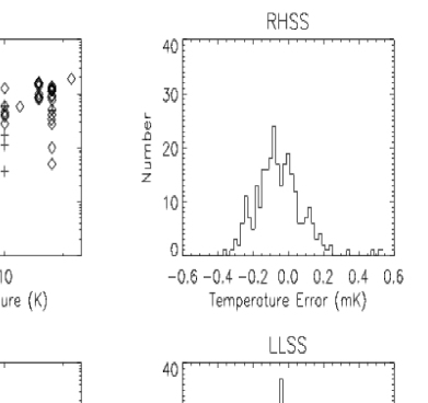
Figure 1: Temperature offset as measured during the FIRAS in-flight calibration, figure taken from [3].

3.1.2 Results for CMB temperature-temperature correlation: WMAP

The WMAP satellite was (among others) designed to observe the angular spectrum of the monopole and the dipole subtracted TT correlator of CMB temperature fluctuations with unprecedented precision. The temperature map underlying this is obtained by comparing the intensity measured for a given direction on the sky and for a given frequency with the respective intensity of an ideal BB. Frequencies considered are contained in one of the bands centered at $\nu=23,33,41,61,$ and 94 GHz. As explained in detail in [15], temperature-temperature correlations extracted from the CMB map practically vanish at large angles ($\theta>60$ degrees) when compared to a prediction based on a scale-invariant spectrum of primordial density perturbations. Also, the low multipoles seem to be statistically correlated which casts doubts on the validity of the usual assumption of statistical isotropy applied when extracting the power of these multipoles.

3.2 Comparison between SU(2)${}_{\tiny\mbox{CMB}}$ and U(1)

Here we would like to present results for the BB spectra and temperature offsets $\delta T$ as they are predicted when replacing the conventional gauge group for photon propagation U(1) by SU(2)${}_{\tiny\mbox{CMB}}$. We define $\delta T\equiv\bar{T}-T$ where the temperature $\bar{T}$ is extracted from a fit of data to the conventional Planck spectrum. This data represents a modified Planck spectrum as generated by SU(2)${}_{\tiny\mbox{CMB}}$ at temperature $T$ ($T$ plays the role of $T_{\tiny\mbox{XCAL}}$ at FIRAS). Both $\bar{T}$ and $T$ are measured in K. The theoretical basis for the postulate SU(2)${}_{\tiny\mbox{CMB}}\stackrel{{\scriptstyle\tiny\mbox{today}}}{{=}}$U(1)_Y and some consequences thereof are discussed in Sec. 2, see also [10, 11, 12, 13, 14, 16].

3.2.1 Embedding of a black body

Before discussing the results of the FIRAS calibration and the WMAP observation we would like to point out the conditions under which the BB anomaly can be detected experimentally.

Strictly speaking, the occurrence of the BB anomaly presumes the absence of conventional, electrically charged matter within the BB cavity (SU(2)${}_{\tiny\mbox{CMB}}$ describes photon propagation only.) A good approximation to this situation is difficult to achieve in terrestial experiments. It is, however, helpful that the effect is predicted to occur for low temperatures where the excitability of residual-gas molecules in the cavity by the BB radiation is very limited. For a measurement in space there is much better vacuum which suggest a cleaner spectral signature.

Let us now address the issue of how temperature offsets $\delta T$ are affected by the embedding of the BB into its surroundings. First we consider the situation of FIRAS. Here a BB is immersed into the surrounding CMB radiation. Compared to the calibration on Earth a larger negative offset of about 4 mK of the radiation temperature as compared to the wall temperature of XCAL was seen during the in-flight calibration ($T_{\tiny\mbox{XCAL}}>T_{\tiny\mbox{CMB}}$).

In our opinion this effect is due to the finite volume of order 1 m³ of the FIRAS instrument and the fact that the correlation length $l(T)$ in the thermal ground state of SU(2)${}_{\tiny\mbox{CMB}}$ is much larger than the linear dimension of the BB cavity at $T_{\tiny\mbox{CMB}}$: $l(T_{\tiny\mbox{CMB}})\sim 1\,\mbox{km}$. In this case, the ground state within the satellite is perceptibly influenced by the ground state of the surroundings because of the large $l$. Going from outside to inside across the BB wall, $l$ is a steeply falling function of distance since the mass of a screened monopole varies rapidly with temperature in the vicinity of $T_{\tiny\mbox{CMB}}$. Radiation emitted from the walls of the BB partially acknowledges the presence of this transition region by loosing part of its energy to the ground state outside the BB. This, in turn, implies a slight reduction of the radiation temperature inside the BB cavity.

But what about the positive temperature offset $\delta T$ of a few mK at $T=2.2\,$K, see Fig. 1? We like to interprete this effect as an increase of the effective number of photon polarizations $F$. Namely, in the case of an infinite BB volume and at $T=2.2\,$K SU(2)${}_{\tiny\mbox{CMB}}$ would be in its confining phase. In the intermediate, preconfining phase the photon would be massive with three polarizations. Since the FIRAS BB has a finite volume and since the ground state of the surrounding Universe has practically an infinite correlation length ($l_{c}\sim 1\,\mbox{km}$) we expect the ground state of the BB cavity to be almost identical to that of the Universe as a whole. That is, the ground state of the BB cavity almost decouples from the excitations, see Sec. 2. A deviation from this situation by tunneling between the pre- and deconfining ground state, which would mean an onset of superconductivity (monopoles are electrically charge w.r.t U(1)_Y) and thus the excitation of a longitudinal photon polarization, is described by a function $f$ of the cavity volume and the correlation length $l$. A quantitative grasp of $f$ would need information about the deviation from the infinite-volume limit considered in [9]. This, however, is beyond the scope of the present work. Due to tunneling a nonvanishing but small probability exists for a photon to possess three instead of two polarizations. As far as BB radiation is concerned, we model this situation by introducing an average number $F$ of photon polarizations which multiplies the conventional Planck spectrum by $F/2$. In Fig. 2 a plot of the (positive) $\delta T$ as a function of $F$ at $T=2.2\,$K is depicted. According to Fig. 2 a typical offset of about 5 mK, compare with Fig. 1, corresponds to about a 1%-increase of the effective number of photon polarizations.

Figure 2: Dependence of the offset $\delta T$ on the effective number of polarizations $F$ at $T=2.2\,$K. The shaded band signals the approximate region for $\delta T$ as measured by FIRAS.

Let us now discuss the situation of a terrestial low-temperature BB experiment. Here the surroundings are at a much higher temperature than $T_{\tiny\mbox{CMB}}$ implying a correlation length $l$ of the external ground state of $l<1\,\mbox{cm}$ [13]. This situation is sketched in the right panel of Fig. 3. Hence in the case of terrestrial FIRAS calibration the warmer ground state of the surroundings had practically no effects on the BB radiation temperature. This would qualitatively explain why the terrestial calibration has seen a much smaller temperature offset $\delta T$ than the in-flight calibration did.

Figure 3: Sketch of the influence of the surrounding’s ground state on the ground state inside the BB cavity. A large correlation length corresponds to in-flight conditions (left panel; small gradient in ground-state energy density represented by dashed line) and a small correlation length to a lab placed on Earth (right panel; large gradient).

3.2.2 Experiment and SU(2)${}_{\tiny\mbox{CMB}}$: FIRAS

The unit of frequency $\nu$ used in the FIRAS experiment is $1\,\mbox{cm}^{-1}$. Since FIRAS has performed most of its BB fits in the range $\nu_{\tiny\mbox{low}}\equiv 1\,\mbox{cm}^{-1}\leq\nu\leq 20\,\mbox{cm}^{-1}\equiv\nu_{\tiny\mbox{up}}$ we will also perform our fits within this range for temperatures up to $T=4\,$K. The reason why we do not consider a fixed value $\nu_{\tiny\mbox{up}}=20\,\mbox{cm}^{-1}$ for temperatures $T$ higher than 4 K is the following. For $T>4\,$K the fits do not saturate when varying $\nu_{\tiny\mbox{up}}$ in the vicinity of $\nu_{\tiny\mbox{up}}=20\,\mbox{cm}^{-1}$. Thus we prescribe $\nu_{\tiny\mbox{up}}=\frac{10}{\mbox{K$\cdot$cm}}\,T$ which is deep inside the saturation regime. In Fig. 4 plots of the dimensionless (in natural units with $c=\hbar=k_{B}=1$) BB spectra are given for both the conventional case and the case of SU(2)${}_{\tiny\mbox{CMB}}$. Notice the regime in frequency of excess (suppression) of spectral power to the right (left) of the critical frequency $\nu^{*}\sim 0.5\,$cm^-1. Suppression is due to photon screening while the excess is caused by antiscreening [11, 12]. Notice also that FIRAS could only observe antiscreening since its value for $\nu_{\tiny\mbox{low}}=1\,\mbox{cm}^{-1}$ is to the right of $\nu^{*}$. A Planck-curve fit to the modified spectrum leads to a negative value of $\delta T$. This is because by Wien’s displacement law a temperature $\bar{T}<T$ is required to account for the larger spectral power at low frequencies. The situation that $\nu^{*}<\nu_{\tiny\mbox{low}}=1\,\mbox{cm}^{-1}$ changes for higher temperatures, see Fig. 5. For example, at $T=20\,$K we have $\nu^{*}>\nu_{\tiny\mbox{low}}$. However, as we will see below, the offset $\delta T$ remains negative for $T\geq 20\,$K. This is explained by the fact that the spectral weight of the screening regime ($\nu<\nu^{*}$) is much lower than that belonging to the regime of antiscreening.

Figure 4: Dimensionless spectral intensity of black-body radiation at $T=5\,$K as described by SU(2)${}_{\tiny\mbox{CMB}}$ (gray curve) and standard U(1) (black curve). The unit of frequency $\nu$ is cm^-1. The left (right) panel depicts the spectrum for $0\leq\nu\leq 97$ cm^-1 (for $0\leq\nu\leq 3$ cm^-1).

Figure 5: Dimensionless spectral intensity of black-body radiation at $T=20\,$K as described by SU(2)${}_{\tiny\mbox{CMB}}$ (gray curve) and standard U(1) (black curve). The unit of frequency $\nu$ is cm^-1. The left (right) panel depicts the spectrum for $0\leq\nu\leq 97$ cm^-1 (for $0\leq\nu\leq 3$ cm^-1).

Let us now discuss the dependence of $\delta T$ on $T$ more quantitatively. Fig. 6 shows the offsets $\delta T$ as a function of T in the range $2.73\,$K$\leq T\leq 100\,$K as extracted by fits involving the dimensionful BB spectra. Fig. 7 shows these offsets when keeping $\nu_{\tiny\mbox{up}}=20\,$cm^-1 fixed as it was done in the FIRAS fit. Obviously, there is growing disagreement between the two plots for $T>4\,$K. This is explained by the smallness of the frequency interval used for generating Fig. 7: The fit gives too much weight to the BB anomaly at low frequencies.

Denoting the statistical error of $\delta T$ by $\Delta T$, the relative statistical error $\frac{\Delta T}{\delta T}$ of the fit grows rapidly with temperature while the $\chi^{2}$/d.o.f. remains comfortably small.

Let us first discuss the case of Fig. 6. At $T=5,7,10\,$ and 20 K we have $\frac{\Delta T}{\delta T}=$25%, 48%, 93%, and 270% and $\chi^{2}$/d.o.f.=2.6$\times 10^{-4}$, 1$\times 10^{-3}$, 5$\times 10^{-3}$, and 4$\times 10^{-2}$, respectively. For $T>80\,$K the $\chi^{2}$/d.o.f. starts to be larger than unity. Judging from the statistical errors, the anomaly is only visible up to $T\sim 10$ K. However, the high quality of the fit, which is expressed by $\chi^{2}$/d.o.f. being substantially smaller than unity, persists up to much larger $T$.

Let us now turn to the statistical errors corresponding to the calibration stage of FIRAS (Fig. 7). Here, we have $\frac{\Delta T}{\delta T}=$25%, 34%, 43%, and 66% and $\chi^{2}$/d.o.f.=6.6$\times 10^{-4}$, 4.4$\times 10^{-3}$, 2.5$\times 10^{-2}$, and 3.9$\times 10^{-1}$ for the same temperatures $T=5,7,10\,$, and 20 K, respectively. Thus the fits are well acceptable from the statistically point of view. Recall, however, that the fitted value for $\delta T$, obtained by keeping $\nu_{\tiny\mbox{up}}$ fixed at $\nu_{\tiny\mbox{up}}=20\,$cm^-1, is not stable under variations in $\nu_{\tiny\mbox{up}}$.

Figure 6: Temperature offset $\delta T$ as a function of $T$ for $2.73\,\mbox{K}\leq\delta T\leq 100\,\mbox{K}$ (left panel) and $2.73\,\mbox{K}\leq\delta T\leq 15\,\mbox{K}$ (right panel). The offset is defined as $\delta T\equiv\bar{T}-T$ where the temperature $\bar{T}$ is extracted by fitting a (dimensionful) U(1) BB-spectrum to a (dimensionful) SU(2)${}_{\tiny\mbox{CMB}}$ BB-spectrum of temperature $T$ within the frequency interval $\nu_{\tiny\mbox{low}}\equiv 1\,\mbox{cm}^{-1}\leq\nu\leq 10\,T\,\mbox{K$\cdot$cm}^{-1}\equiv\nu_{\tiny\mbox{up}}$. For the fit we have used 5000 equidistant frequency points in this interval.

Figure 7: Same as in Fig 6 but now keeping $\nu_{\tiny\mbox{up}}$ fixed at 20 cm^-1.

3.2.3 Observation and SU(2)${}_{\tiny\mbox{CMB}}$: WMAP

Let us now discuss our results adapted to the conditions of CMB observations carried out by the WMAP mission. In the Table we give the frequency bands used by WMAP [7] for the generation of the dipole- and monopole subtracted map of temperature fluctuations over the sky.

band	$\nu_{\mathrm{low}}$ [GHz]	$\nu_{\mathrm{up}}$ [GHz]	$\nu_{\mathrm{low}}$ [cm-1]	$\nu_{\mathrm{up}}$ [cm-1]
K	19.5	25	0.65	0.83
Ka	28	37	0.93	1.23
Q	35	46	1.17	1.53
V	53	69	1.77	2.30
W	82	106	2.74	3.54

Figure 8: Offset $\delta T$ as a function of $T$ for $2.73\,\mbox{K}\leq\delta T\leq 30\,\mbox{K}$. The offset is defined as $\delta T\equiv\bar{T}-T$ where the temperature $\bar{T}$ is extracted by fitting a (dimensionful) U(1) BB-spectrum to a (dimensionful) SU(2)${}_{\tiny\mbox{CMB}}$ BB-spectrum of temperature $T$ within the frequency of the blueshifted WMAP frequency bands, see text. For the fit we have used 1000 equidistant points within each of the five WMAP frequency bands.

Our goal is to extract the offsets $\delta T\equiv\bar{T}-T$ in analogy to Sec. 3.2.2. We now perform the fits within all blueshifted WMAP frequency bands. Notice that these frequency bands lie deep inside the Raleigh-Jeans regime of the BB spectrum. By blueshift we mean that the frequencies in the WMAP bands are rescaled by a factor of $T/(2.73\,\mbox{K})$. This corresponds to a fictitious WMAP observation of the associated BB intensity in an earlier Universe at redshift $z=T/(2.73\,\mbox{K})-1$. Within each frequency band we use 1000 equidistant points.

Although a direct comparison of the temperature offsets, extracted under the above conditions, with the $TT$ angular correlation functions as extracted from the WMAP temperature map is impossible, we may however discuss some qualitative features of Fig. 8. First, notice the change in sign at a redshift $z$ of about $z=1$. This change in sign is accompanied with a strong gradient. In [16] it was shown that the bulk of the contribution to the dynamical component to the CMB dipole is generated around $z=1$. By inspecting Fig. 8 we observe a large slope in the $z$-evolution of $\delta T$ around $z=1$. This implies a rapid built-up of a temperature profile out of an initial inhomogeneity at this redshift. Second, notice the decreasing slope of $\delta T(z)$ for increasing values of $z>1$. In this regime the built-up of inhomogeneities is much weaker than in the vicinity of $z=1$.

Figure 9: Offset $\delta T$ as a function of $T$ for $2.73\,\mbox{K}\leq\delta T\leq 100\,\mbox{K}$ when using the Stefan-Boltzmann law as a model for the fit of the total energy density. The offset is defined as $\delta T\equiv\bar{T}-T$ where $\bar{T}$ is the conventional BB temperature attributed to the integral over the modified BB spectrum.

Thus there is no major modification of the primordial spectrum associated with evolution down to $z\sim 1$. Due to the rapid built-up of the dipole contribution at $z=1$ pre-existing, large angle fluctuations are smoothed (inflated) away and get statistically correlated with the dipole. Based on the work in [16], we will make this assertion much more quantitative in a forthcoming publication [19]. Finally, notice that the values for $\delta T$ at a given temperature are quite different in the case of a FIRAS-like and WMAP-like extraction. For example, at $T=6.83$ K we have $\delta T=-1.44\times 10^{-3}$ K from WMAP and $\delta T=-0.085\times 10^{-3}$ K from FIRAS when performing the fit in the range $\nu_{\mathrm{low}}=1\,$cm${}^{-1}\leq\nu\leq 10\,T\,\mbox{K$\cdot$cm}^{-1}\equiv\nu_{\tiny\mbox{up}}$.

3.2.4 Temperature offsets from Stefan-Boltzmann law

After having discussed the emergence of temperature offsets $\delta T$ when fitting modified to conventional BB spectra we now point out the differences of this method as compared to the extraction of $\delta T$ from integrated spectra (integration over all frequencies). The model now is that the Stefan-Boltzmann law $\rho=\mbox{const}\,T^{4}$ shall hold for the integral $\rho_{\tiny\mbox{con}}$ over the conventional BB spectrum as well as for the integral $\rho_{\tiny\mbox{mod}}$ over the modified BB spectrum. To linear order in $\delta T$ we thus have

$$\delta T\equiv\bar{T}-T=T\,\frac{\rho_{\tiny\mbox{mod}}-\rho_{\tiny\mbox{con}}}{4\rho_{\tiny\mbox{con}}}\,.$$ (9)

In Fig. 9 we show a plot of $\delta T$ as extracted from Eq. (9). Comparing Figs. 9, 6 and 8, we observe that the sign of $\delta T$ does not coincide for sufficiently high temperatures. On one hand, the positivity of $\delta T$, as extracted from Eq. (9), is explained by the regime of antiscreening having a larger weight in the integration of the modified BB spectrum than the regime of screening. On the other hand, the fit to the BB spectrum interpretes the regime of antiscreening in terms of a decrease of temperature in accord with Wien’s displacement law. So the two methods produce even qualitatively different results.

4 Summary and Conclusions

In this article we have performed an analysis of offsets between radiation- and wall-temperatures in ideal black bodies. On the theoretical side these offsets arise due to nonabelian effects of an SU(2) Yang-Mills theory of scale $\Lambda=10^{-4}$ eV [11, 12, 13, 14]: SU(2)${}_{\tiny\mbox{CMB}}$. The deviation from the conventional black-body spectra peak at temperatures a few times that of the present cosmic microwave background. There are two ways of extracting these temperature offsets: Either assume a Stefan-Boltzmann form of the energy density (integrated, modified black-body spectrum) or assume a conventional black-body spectral shape as fit models for the data representing the modified spectrum. For the frequency ranges and the frequency bands used in the FIRAS instrument calibration and in the WMAP mission, respectively, we have extracted these offsets using the latter method. We find that in the case of FIRAS the nonabelian effects, as predicted by SU(2)${}_{\tiny\mbox{CMB}}$, are too small to rise above the errors of the experiment. We give qualitative explanations for the global, negative offset of about $-4\,$mK observed for in-flight calibration at temperatures larger than $T_{\tiny\mbox{CMB}}=2.73\,$K and the positive offset for calibration at $T=2.2\,$K. Both effects are further evidence toward the correctness of the postulate that photon propagation is described SU(2)${}_{\tiny\mbox{CMB}}$. In order to verify or falsify this postulate a terrestrial low-temperature, low-frequency, high-precision measurement of the black body spectral intensity surely is required. We are confident, however, that work performed in the framework of [16] will yield the suppression and correlation of the low-lying CMB multipoles [19] as extractable from the data of the WMAP mission [15].

Comparing our result for the FIRAS and the WMAP setting, we obtain offsets that are larger by an order of magnitude for the spectral fits in the blueshifted frequency bands of the latter. Interestingly, the value of the minimum in the WMAP fit, which occurs at a temperature corresponding to a redshift $z=1.5$, is close in magnitude to the amplitude of the (dynamical component of the) dipole, for a discussion see [16]. Furthermore, the large slope of $\delta T(z)$ in the vicinity of $z=1$ very likely is associated with the rapid built-up of the dynamical component of the CMB dipole. This process implies a smoothing of primordial, large-angle fluctuations and a correlation thereof. We will make this assertion much more quantitative in a forthcoming publication [19].

Finally, for the extraction of $\delta T$ from presuming the Stefan-Boltzmann law we observe vast deviations compared to the extraction from spectral fits. This is true for both magnitude and sign. Thus to speak of temperature offsets generated by whatever possible mechanism it is imperative to specify the method used to extract them.

References

- [1] G. Gamow, Phys. Rev. 70, 572 (1946).
- [2] A. A. Penzias and R. W. Wilson, Astrophys. J. 142, 419 (1965).
- [3] FIRAS Explanatory Supplement, edited by Brodd et al., available at http://lambda.gsfc.nasa.gov/product/cobe/firas-exsupv4.cfm.
- [4] D. J. Fixsen et al., Astrophys. J. 420, 457 (1994).
- [5] J. C. Mather et al., Astrophys. J. 420, 439 (1994).
- [6] J. C. Mather et al., Astrophys. J. 512, 511 (1999).
- [7] Wilkinson Microwave Anisotropy (WMAP): Three-Year Explanatory Supplement, editor M. Limon, et al. (Greenbelt, MD:NASA/GSFC) Available in electronic form at http://lambda.gsfc.nasa.gov
- [8] G. Hinshaw et al., astro-ph/0603451.
-
[9]
R. Hofmann, Int. J. Mod. Phys. A20, 4123 (2005), Erratum-ibid A21, 6515 (2006) [hep-th/0504064].
R. Hofmann, Mod. Phys. Lett. A21, 999 (2006), Erratum-ibid. A 21, 3049 (2006) [hep-th/0603241]. - [10] R. Hofmann, PoS JHW2005, 021 (2006) [hep-ph/0508176].
- [11] M. Schwarz, R. Hofmann, and F. Giacosa, Int. J. Mod. Phys. A 22, 1213 (2007) [hep-th/0603078].
- [12] M. Schwarz, R. Hofmann, and F. Giacosa, JHEP 0702, 091 (2007) [hep-ph/0603174].
-
[13]
R. Hofmann, Int. J. Mod. Phys. A20, 4123 (2005), Erratum-ibid A21, 6515 (2006) [hep-th/0504064].
R. Hofmann, Mod. Phys. Lett. A21, 999 (2006), Erratum-ibid. A 21, 3049 (2006) [hep-th/0603241].
F. Giacosa and R. Hofmann, hep-th/0609172.
R. Hofmann, hep-th/0609033. - [14] F. Giacosa and R. Hofmann, Eur. Phys. J. C50, 635 (2007) [hep-th/0512184].
- [15] C. Copi, D. Huterer, D. Schwarz, and G. Starkman, Phys. Rev. D 75, 023507 (2007) [astro-ph/0605135].
- [16] M. Szopa and R. Hofmann, hep-ph/0703119.
- [17] F. Giacosa and R. Hofmann, hep-th/0703127.
-
[18]
D. Miller, Phys. Rept. 443, 55 (2007) [hep-ph/0608234].
D. Miller, Act. Phys. Pol. B 28, 2937 (1997). - [19] M. Szopa, R. Hofmann, and F. Giacosa, work in progress.