Quasifree $\Lambda$, $\Sigma^{0}$, and $\Sigma^{-}$ electroproduction from ^1,2H, ^3,4He, and carbon

Abstract

Kaon electroproduction from light nuclei and hydrogen, using ¹H, ²H, ³He, ⁴He, and carbon targets has been measured at Jefferson Laboratory. The quasifree angular distributions of $\Lambda$ and $\Sigma$ hyperons were determined at $Q^{2}=0.35$ (GeV/c)² and $W=1.91$ GeV. Electroproduction on hydrogen was measured at the same kinematics for reference.

Introduction

A comprehensive study of kaon electroproduction on light nuclei has been conducted in Hall C of Thomas Jefferson National Accelerator Facility (Jefferson Lab or JLab). Data were obtained using electron beams of 3.245 GeV impinging on special high density cryogenic targets for, ^1,2H, ^3,4He, as well as on a solid carbon target.

Until recently the data base of cross sections of electro- and photoproduction of strangeness was sparse. In the case of photoproduction, considerable amounts of new high quality data for the proton have been published from experiments at JLab, ELSA, SPring-8, GRAAL and LNS (cf. Dohrmann (2006) for a list of references). These data include cross sections, polarization asymmetries, tensor polarizations, and decay angle distributions. However, the data base for photoproduction on nuclei and thus implicitly the neutron remains scarce (cf. Kohri et al. (2006); Niculescu (2001)). Only few older measurements have been reported on deuterium Boyarski et al. (1976); Quinn et al. (1979) and carbon Yamazaki et al. (1995) targets.

Traditionally, ²H and ³He targets have been considered to be a good approximation for a free neutron target. In the present work, as in the majority of kaon electroproduction experiments, a positive kaon is detected in coincidence with the scattered electron. On the proton, this leads to two possible final states with either a $\Lambda$ of $\Sigma^{0}$ hyperon, that are easily separable by a missing mass analysis. On the neutron, a $\Sigma^{-}$ is produced as final state. Due to the small mass difference of $\Sigma^{-}$ and $\Sigma^{0}$ of 4.8 MeV/c² and the initial nucleon momentum distribution, the $\Sigma$ contributions from the proton and neutron cannot be separated by missing mass. With increasing target mass, the separation between $\Lambda$ and $\Sigma$ distributions also gets worse because of the increasing Fermi momentum. Thus, ²H and ³He targets offer the best access to the neutron cross sections. Since a missing mass analysis, strictly speaking, can only determine the total $\Sigma$ strength, the different $N/Z$ ratio for the ²H and ³He targets should assist in further disentangling the $\Sigma^{0}$ and $\Sigma^{-}$ contributions.

Systematic studies of heavier nuclei will then provide the possibilities of investigating in-medium modifications of the elementary kaon electroproduction mechanism as well as the propagation of the outgoing $K^{+}$. e.g. experimental data on ¹²C Yamazaki et al. (1995); Hinton (1998); Miyoshi et al. (2003); Yuan et al. (2006) show an effective proton number that is in disagreement with theoretical calculations Lee et al. (1998), thereby indicating the need for modifications.

We present here the results of an experiment on the electroproduction of open strangeness on light nuclei with $A=2,3,4,12$, that has been performed in Hall C at Jefferson Lab. Also measured was the production on a hydrogen target. This facilitates direct comparison to the elementary $p(e,e^{\prime}K^{+})$ reaction for identical kinematics. Results of this experiment on the production of $\Lambda$ hypernuclear states, ${}^{3}_{\Lambda}\mathrm{H}$ and ${}^{4}_{\Lambda}\mathrm{H}$, have been presented in Ref. Dohrmann et al. (2004). In this paper we present the cross sections for the quasifree production of $\Lambda$, $\Sigma^{0}$, $\Sigma^{-}$. To the best knowledge of the authors, this is the first reported kaon electroproduction measurement on helium isotopes.

Experiment

Experiment E91-016 had two runs, one that only used Hydrogen and Deuterium targets, and a subsequent one that also included helium and carbon targets. We present cross sections from the second run, which included data for all four few-body nuclei. Data were obtained using electron beams of 3.245 GeV impinging on special high density cryogenic targets for ^1,2H, ^3,4He. The target thicknesses were 289 mg/cm² for ¹H at 19 K, 668 mg/cm² for ²H at 22 K, 310 mg/cm² for ³He at 5.5 K, and 546 mg/cm² for ⁴He at 5.5 K. The target lengths were approximately 4 cm for each target. In addition, data was taken on a 227 mg/cm² carbon target.

The scattered electrons were detected in the High Momentum Spectrometer (HMS, momentum acceptance $\Delta p/p\approx\pm 10\%$, solid angle $\approx 6.7$ msr) in coincidence with the electroproduced kaons, detected in the Short Orbit Spectrometer (SOS, momentum acceptance $\Delta p/p\approx\pm 20\%$, solid angle $\approx 7.5$ msr). The detectors and coincidence methods have been described in detail for similar experiments in Hall C Mohring et al. (2003); Gaskell et al. (2002); Dutta et al. (2003). The detector packages of the two spectrometers are very similar, and a sketch of the setup of the experiment is shown in Fig. 1. Two drift chambers near the focal plane, used for reconstructing the particle trajectories, are followed by two pairs of segmented plastic scintillators that provide the main trigger signal as well as the time-of-flight information. The time-of-flight resolution is $\sim 150$ ps $(\sigma)$. For electron identification, a lead-glass shower detector array together with a gas threshold Čerenkov is used in order to distinguish between $e^{-}$ and $\pi^{-}$. For kaon identification in the SOS, a silica aerogel detector (n=1.034) provided $K^{+}/\pi^{+}$ discrimination while an acrylic Čerenkov counter (n=1.49) was used for $K^{+}/p$ discrimination.

Electroproduction processes involve the exchange of a virtual photon, $\gamma^{*}$, between projectile and target. The spectrometer setting for electron detection was kept fixed at an angle of 14.93^∘ during the experiment, thereby holding the virtual photon flux constant (cf. Ref. Zeidman et al. (2001)). The initial spectrometer angle of the kaon arm was $13.40{{}^{\circ}}$. This angle was varied to measure angular distributions with respect to the direction of $\gamma^{*}$. For the $\gamma^{*}$, the invariant mass was $Q^{2}=0.35$ (GeV/c)², the virtual photon momentum was $|\vec{q}|=1.77$ GeV/c and the total energy in the photon-nucleon system was $W=1.91$ GeV. Electroproduction on light nuclei was studied for three different angle settings with respect to the initial kaon angle, $13.40{{}^{\circ}}$. The corresponding angle between the virtual photon, $\gamma^{*}$ and the ejected kaon ($K$), are $\theta_{\gamma^{*}K^{+}}^{\mathrm{lab}}\simeq 1.7{{}^{\circ}},~{}6{{}^{\circ}},~{}12{{}^{\circ}}$. These correspond to increasing the momentum transfer to the hyperon ($\mid t\mid\simeq(0.12,\;0.14,\;0.23)\;\mathrm{GeV}^{2}$). The central spectrometer momenta were 1.29 GeV/c for the kaon arm and 1.57 GeV/c for the electron arm.

Data analysis

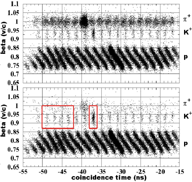
Figure 2: (Color online) Real and random events of $\beta_{K^{+}}$ versus the path-length corrected coincidence time measured by the SOS spectrometer. Visible bands correspond to protons (low velocities), kaons and pions (high velocities). The tilt of the pion and proton bands reflects that $\beta$ was calculated assuming the particle was a kaon. The effect of PID cuts, is shown in the bottom figure, where the fast pions were almost totally removed. The random events are determined by averaging over a number of random coincidence peaks as indicated by the large red box. These are to be subtracted from the small red box around the main coincidence peak.

The essential element of the data analysis for the present work is a clear identification of scattered electrons coincident with kaons against a large background of pions and protons. Figure 2 shows the measured hadron velocity in the SOS versus the coincidence time between the two spectrometers. The latter has been projected back to the target by using the kaon mass as default. It thus represents the proper coincidence time only for kaons, the particles of interest. Clearly visible is the 2-ns RF time structure of the beam. The top panel shows the distributions before, the bottom panel after applying an analysis cut on the aerogel Čerenkov detector. In-time electron-kaon coincidences are selected by a cut on $\beta$ and coincidence time. The background from uncorrelated $(e,K^{+})$ pairs was subtracted using distributions from out-of-time coincidences, a standard procedure for Jefferson Lab Hall C experimentsGaskell et al. (2002); Ambrozewicz et al. (2004). Defining the out-of-time window such that it does not include any in-time coincidences of $(e,\pi)$ and $(e,p)$, this procedure also corrects for any remaining pion and proton background in the in-time kaon window.

Following Ref. Knöchlein et al. (1995); Janssen (2002), the notation of strangeness electroproduction may be introduced by

$$p(p^{\mu})+e(q^{\mu}_{e})\to e^{\prime}(q^{\mu}_{e^{\prime}})+K(p^{\mu}_{K})+Y(p^{\mu}_{Y}),$$ (1)

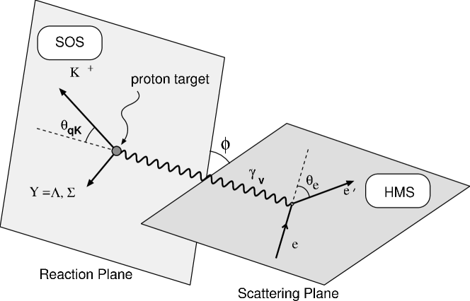
Figure 3: The kinematics of kaon electroproduction: the reaction (hadron) and scattering (lepton) planes are connected by the virtual photon which lies in both planes. The electron scattering angle is denoted by $\theta_{e}$, the kaon scattering angle between the kaon and the direction of the virtual photon is denoted by $\theta_{\gamma K}$. Typically for electroproduction experiments in Hall C of JLab, the ejected $K^{+}$ was detected by the SOS spectrometer in coincidence with the scattered $e^{\prime}$, detected by the HMS spectrometer [from Mohring et al. (2003)].

with the four-momenta $q^{\mu}_{e}=(E_{e},\vec{q}_{e})$, $q^{\mu}_{e^{\prime}}=(E_{e^{\prime}},\vec{q}_{e^{\prime}})$ of the incoming and outgoing electron, $q^{\mu}=(\omega,\vec{q})$ of the virtual photon, $p^{\mu}_{p}=(E_{p},-\vec{q})$, $p^{\mu}_{K}=(E_{K},\vec{p}_{K})$, $p^{\mu}_{Y}=(E_{Y},-\vec{p}_{K})$. The virtual photon is defined by the difference of the four-vectors of the incoming and outgoing electron, $q^{\mu}=q^{\mu}_{e}-q^{\mu}_{e^{\prime}}$. The kinematics are shown in Fig. 3, where the lepton and hadron planes are defined. The virtual photon connects both planes kinematically.

After proper electron and kaon identification, the measured momenta (magnitude and direction with respect to the incoming beam) allow for a full reconstruction of the missing energy and missing momentum of the recoiling system:

The missing energy and missing momentum of the recoiling nucleons are calculated viz. 

$$E_{X} =E_{e}-E_{e^{\prime}}+M_{\mathrm{targ}}-E_{K}=\omega+M_{\mathrm{targ}}-E_{K},$$ (2)

$$\vec{P}_{X} =\vec{q}-\vec{p}_{K},$$ (3)

where $M_{X}=\sqrt{(E_{X}^{2}-|\vec{P}_{X}|^{2})}$ is the missing mass, $M_{\mathrm{targ}}$ denotes the target mass. The four-momentum transfer to the nucleons is given by the Mandelstam variable $t$,

$$t=(q^{\mu}-p_{K}^{\mu})^{2}=(\omega-E_{K})^{2}-|\vec{q}|^{2}-|\vec{P}_{K}|^{2}+2|\vec{q}||\vec{P}_{K}|\cos{\theta_{pK}}\,.$$ (4)

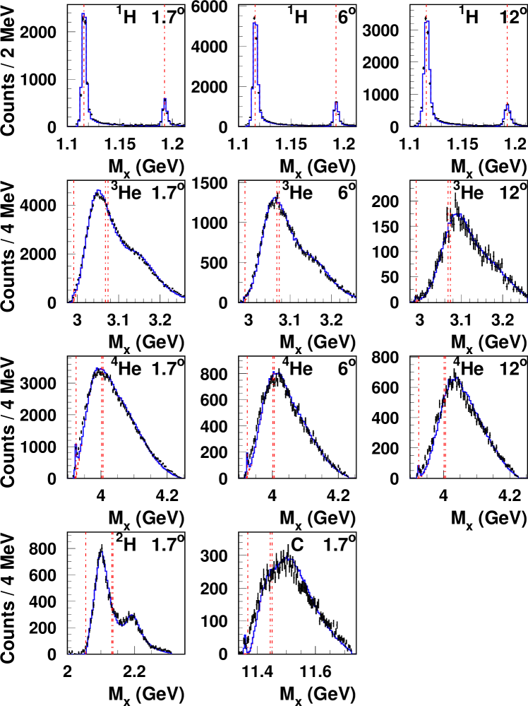
Figure 4: (Color online) Reconstructed missing mass spectra for all five targets at all kinematic settings as indicated. For ${}^{1}H$, ³He, ⁴He, three kinematic settings were measured, whereas for ${}^{2}H$, and C targets only one kinematic setting ($1.7^{{{}^{\circ}}}$) was measured. The blue line represents the respective fit to each spectrum.

Final states of the $A(e,e^{\prime}K)X$ reaction for $A=1,2,3,4,12$ are visible in Fig. 4. The missing mass $M_{X}$ is calculated from the four momenta $q^{\mu}$ of the virtual photon and the four momentum $p^{\mu}_{K}$ of the detected kaon, viz. 

$$M_{X}^{2}=(q^{\mu}+P_{\mathrm{targ}}^{\mu}-p_{K}^{\mu})^{2},$$ (5)

where $P^{\mu}_{\mathrm{targ}}=(M_{\mathrm{targ}},0,0,0)$ is the target four-momentum.

Missing mass distributions have been created for the in-time (e,K) coincidences as well as a sample of the out-of-time coincidences; the latter then were subtracted with the appropriate weight. For the cryogenic targets, the background from the target cell walls was determined by a measurement from an empty cell replica. Data from this replica were subjected to the same analysis and subtracted from the distributions.

Figure 4 shows background subtracted missing mass distributions for all four targets. For the hydrogen target, the missing mass distributions allow for an unambiguous identification of the electroproduced hyperon, either a $\Lambda$ or a $\Sigma^{0}$. The well known masses of these two hyperons also serve as an absolute mass calibration with an accuracy of better than 2 MeV.

On the deuterium target, the two distributions are significantly broadened because of the presence of a nucleon spectator and the Fermi motion of the target nucleons. Furthermore, the $\Sigma$ distribution now is comprised of two possible final states, either a $\Sigma^{0}n$ or a $\Sigma^{-}p$; the latter from the reaction with a neutron inside the target. Since the mass difference between $\Sigma^{0}$ and $\Sigma^{-}$ is small compared to the width of the distributions, these two final states are completely unresolved. In Fig. 4 it is also obvious that the radiative tail from the $\Lambda$ distribution contributes significantly to the strength observed in the $\Sigma$ mass region. For increasing $A$, the peaks associated with $\Lambda$ and $\Sigma$ hyperons further broaden. Whereas for ³He a small shoulder associated with $\Sigma$ is still visible, only an indistinct broad distribution remains for the ⁴He target.

This challenges any extraction of the underlying three reaction channels $\gamma^{*}+p\to\Lambda+K^{+}$, $\gamma^{*}+p\to\Sigma^{0}+K^{+}$, and $\gamma^{*}+n\to\Sigma^{-}+K^{+}$. The following section will describe an attempt to disentangle the three reaction channels by means of a Monte Carlo simulation that models the spectrometer acceptances as well as the reaction mechanism.

The electroproduction cross section may be written as follows:

$$\frac{d^{5}\sigma}{dE_{e^{\prime}}d\Omega_{e^{\prime}}d\Omega_{K}}=\Gamma\frac{d^{2}\sigma}{d\Omega_{K}}$$ (6)

where $\Gamma$ denotes the virtual photon flux factor:

$$\Gamma=\frac{\alpha}{2\pi^{2}}\frac{E_{e^{\prime}}}{E_{e}}\frac{1}{Q^{2}}\frac{W^{2}-M^{2}}{M}\frac{1}{1-\varepsilon},$$ (7)

where $\alpha$ is the fine structure constant and $\varepsilon$ is the longitudinal polarization of the virtual photon,

$$\varepsilon=\left(1+2\frac{|\vec{q}|^{2}}{Q^{2}}\tan^{2}(\theta_{e}/2)\right)^{-1}.$$ (8)

The total energy in the virtual photon–target center is given by $W^{2}=s=(q^{\mu}+p^{\mu}_{\mathrm{target}})^{2}$ and can be expressed in the laboratory reference frame by $W^{2}=M^{2}+2M\omega-Q^{2}$. To facilitate comparison with the scattering on the proton, both for calculating $W$ as well as in Eq. (7) $M$ is taken to be the nucleon mass for all targets discussed here.

The ${}^{1}\mathrm{H}(e,e^{\prime}K^{+})X$ data was used to provide consistent normalization data as well as to test available isobar models and to develop a global model that would describe the data. While reasonable agreement was found with the Saclay-Lyon model David et al. (1996), the best description of the data within the kinematic range of this experiment was achieved by a dedicated simple model. This model had already been developed for the first experimental run on $A=1,2$ targets Cha (2000). Unlike the Saclay-Lyon model it is not based on separated response functions. Instead the unpolarized two-fold center of mass cross section is modeled and taken as input for the simulations, which then provides a five-fold laboratory cross section as output.

The model describes the unpolarized differential cross section for ${}^{1}\mathrm{H}(e,e^{\prime}K^{+})\Lambda$ by a factorization ansatz of four kinematic variables:

$$\left.\frac{d^{2}\sigma}{d\Omega}\right|_{\Lambda}\left(Q^{2},W,t,\phi\right)=f(Q^{2})\times N\cdot g(W)h(t)i(\phi),$$ (9)

with a normalization constant $N=5.4724$ and the four functions

$$f(Q^{2}) =\mathrm{constant}=c_{1}^{f},$$ (10)

$$g(W) =c^{g}_{1}\frac{P_{K}^{\mathrm{cm}}}{(W^{2}-M_{p}^{2})W}+$$

$$+c^{g}_{2}\frac{W^{2}}{c^{g}_{3}W^{2}+(W^{2}-1.72^{2})^{2}},$$ (11)

$$h(t_{\mathrm{min}}-t) =\exp(c^{h}_{1}(t_{\mathrm{min}}-t)),$$ (12)

$$i(\phi) =c_{1}^{i}+c_{2}^{i}\cos(\phi)+c_{3}^{i}\cos(2\phi).$$ (13)

The $c_{1,2,3}^{f,g,h,i}$ are parameters which are determined through a fit to the data taken during the first experimental run Cha (2000); Reinhold et al. (2001). These parameters are given in Table 1.

The functional form of the t dependence in Eq. (12) has been taken from an earlier work by Brauel et al. Brauel et al. (1979), while the $\phi$ dependence was studied during the first run of the experiment Cha (2000). Equation (11) shows that the dependence on the total photon energy $W$ is composed of a phase space factor and a Breit-Wigner resonance. The observed $Q^{2}$ dependence is very weak and it is set to a constant.

For the electroproduction of $\Sigma^{0}$ hyperons, ${}^{1}\mathrm{H}(e,e^{\prime}K^{+})\Sigma^{0}$, only a single, energy dependent phase space factor is used. Following Bebek et al. (1977) we obtain

$$\left.\frac{d^{2}\sigma}{d\Omega}\right|_{\Sigma}\left(W\right)=c_{1}\frac{P_{K}^{\mathrm{cm}}}{(W^{2}-M_{p}^{2})W};\quad c_{1}=1.32\,\mathrm{GeV}^{2}\mu\mathrm{b/sr}$$ (14)

where the constant $c_{1}$ was determined by Koltenuk Koltenuk (1999).

Unlike hydrogen, the missing mass distributions for deuterium and the other nuclear targets do not show two clearly separable peaks, cf. Fig. 4, as discussed above. To extract information on the quasifree $\Sigma^{0}$ as well as $\Sigma^{-}$ production, one has to rely on assumptions about the nuclear dependence of the $\Sigma^{0}$. In this analysis, we determine the ratio of $\Lambda$ to $\Sigma$ production for hydrogen and then keep this ratio fixed in the proton model that enters into the simulation for the nuclear cross section. Nuclear effects thus contribute to the systematic uncertainties (cf Abbott et al. (1998); Kohri et al. (2006)). If such an assumption is not made, only a combined $\Sigma$ contribution may be deduced, as in Boyarski et al. (1971); Quinn et al. (1979).

The data shown in Fig. 4 were compared with a dedicated Monte Carlo simulation that modeled the spectrometer optics and acceptance, kaon decay, small angle scattering, energy loss and radiative corrections Ent et al. (2001); Mohring et al. (2003). The process of extracting the respective cross sections described in detail in Ambrozewicz et al. (2004); Gaskell et al. (2002), relies upon a ratio of the measured yield from experiment, $Y_{\mathrm{exp}}$, normalized to a simulated yield from the above mentioned Monte Carlo simulation, $Y_{\mathrm{MC}}$, which is used as a scale factor for the model cross section used in the Monte Carlo, viz. 

$$\frac{d^{2}\sigma}{d\Omega}=\frac{Y_{\mathrm{exp}}}{Y_{MC}}\cdot\left.\frac{d^{2}\sigma}{d\Omega}\right|_{\mathrm{model}}.$$ (15)

This approach is also known as the method of correction factors, cf. Cowan (1998). For $A=2,3,4,12$ the $A(e,e^{\prime}K^{+})X$ process was modeled as quasifree scattering on target nucleons inside the target. Since to the best knowledge of the authors no dedicated models are available for the electroproduction on these nuclei, the elementary cross section model eqs. (9)–(13) for $\Lambda$ and eq. (14) for $\Sigma$, are used. The respective cross sections are multiplied by the number of protons, $Z$, or neutrons, $N$, respectively. Since no separate model for the production on the neutron is available, we use the model (14) for both $\Sigma^{0}$ as well as $\Sigma^{-}$. The model is convolved with spectral functions Benhar et al. (1994) for the respective target nucleus.

The spectral functions provide the four-momenta of the target nucleons inside the target. For the $A=2$ case, deuteron momentum distributions taken from either the Bonn potential Machleidt et al. (1987) or the Av18 potential Wiringa et al. (1995) gave essentially identical results. Obviously neither of these models incorporate any possible in-medium behavior of the nucleons inside the target nor final state interaction as will be discussed below. For the nuclear targets, final state interactions in the vicinity of the respective quasifree thresholds are taken into account using an effective range approximation Gillespie (1964).

The final state interaction of the hyperon with the remaining target nucleon has to be taken into account, whereas the kaon nucleon final state interaction is small; the $\Lambda N$ total cross section is more than two orders of magnitude larger than the $K^{+}N$ total cross section. We use an effective range approximation (ERA), by which the modeled cross section is modified by an enhancement factor $I$ (cf. Watson and Migdal Watson (1952); Migdal (1955)),

$$\sigma_{K}^{YN\,\mathrm{FSI}}=I\sigma_{K}=\frac{1}{|J_{l}(k_{\mathrm{rel}})|^{2}}\cdot\sigma_{K},$$ (16)

in terms of the complex Jost function $J_{l}$ for the $l$th partial wave. $k_{\mathrm{rel}}$ is the relative momentum between the hyperon and the nucleon (see also chapters 12 and 14 of Newton (1982)). A hyperon–nucleon ($YN$) potential $V$ is used to describe the final state interaction, for which only the s-wave part is taken into account. The s-wave Jost function may then be written as

$$J(k_{\mathrm{rel}})=\frac{k_{\mathrm{rel}}-i\beta}{k_{\mathrm{rel}}-i\alpha},$$ (17)

where $\alpha$ and $\beta$ are determined from the scattering length $a$ and effective range $r_{e}$ of the hyperon-nucleon potential viz. 

$$\frac{1}{2}r_{e}(\alpha-\beta)=1\,,\quad\frac{1}{2}r_{e}\alpha\beta=-\frac{1}{a}\,.$$ (18)

In this ansatz there are no free parameters, the magnitude of the enhancement factor is fully determined by the effective range $r_{e}$ and the corresponding scattering length $a$, both being parameters of the hyperon-nucleon potential chosen. For the $A=2$ targets, the full Jost function ansatz gave a less satisfactory description of the data than for the helium targets. An even simpler approach for an ERA, studied in Cha (2000) and following a prescription described in reference Li and Wright (1991) was used. The s-wave phase shift $\delta_{0}$ is calculated via the Bethe formula and the enhancement factor is given by

$$k_{\mathrm{rel}}\cot\delta_{0}=-\frac{1}{a}+0.5r_{e}k_{\mathrm{rel}}^{2}\quad I=\left(\frac{\sin(\delta_{0}+k_{\mathrm{rel}}r)}{\sin{k_{\mathrm{rel}}r}}\right)^{2}.$$ (19)

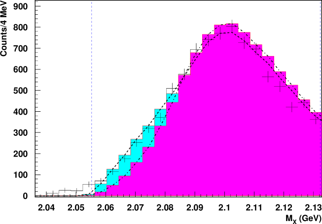
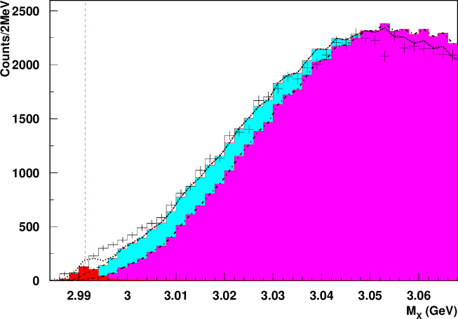
Figure 5: (Color online) The effects of including FSI for the fits to the data on ²H (upper panel) and ³He (lower panel) in the low-mass $\Lambda$ region. The fitted $\Lambda$ contribution without FSI is given by the dark color, dash-dotted line. $\Lambda$ contributions including FSI are given by the light-blue, dashed line. For ³He, the ${}^{3}_{\Lambda}$H bound state is shown in red. The total fit (sum of all contributions) is given by the dotted line. The vertical dashed line denotes the threshold for $\Lambda$ production on ² H, ³He, respectively.

For the helium targets, however, the full Jost function ansatz gave much better results. For the data sets presented in this paper, we use the Nijmegen 97f $YN$ potential Rijken et al. (1999), with scattering lengths $a$ taken from Rijken et al. (1999) and effective ranges of $r_{e}$ taken from the Nijmegen 89Maessen et al. (1989), since Ref. Rijken et al. (1999) does not provide these parameters. In all cases and for every hyperon–nucleon potential tested, the singlet values for $a$ and $r_{e}$ gave more satisfactory results than triplet values. For the $\Sigma$ hyperons, the Nijmegen 97f and the Jülich A also provide $a$ and $r_{e}$ for the $\Sigma N$ interaction. Using these values, an enhancement factor due to $\Sigma N$ final state interaction was introduced. However, the fits to the data were more strongly influenced by the $\Lambda N$ final state interaction. In Fig. 5 we show the effect of applying final state interaction in an ERA to our model in the low-mass $\Lambda$ region.

In Table 2 we show the influence of the FSI on the simulated missing mass yields. The simulated missing mass is weighted by the respective model cross section. If the cross section is multiplied by an enhancement factor, the missing mass spectra is influenced. Table 2 gives the ratio of the integrated yields $Y_{\mathrm{FSI}}/Y_{\mathrm{no\_FSI}}$ for missing mass distributions (cf. Figs. 4 and 6) with or without FSI for the model (9) discussed above. Choosing a different cross section model would change these values only by 1%–3%. cross section models. Also, different final state interaction models (e.g. Nijmegen 97f, Jülich A) do not change the yield ratio by more than 3%.

For the helium-3 and helium-4 target nuclei (and also for carbon), the analysis was performed analogously to the $A=2$ case. However, the electroproduction of strangeness on helium targets (and on carbon, though with a rather poor statistics) triggers two investigations: the quasifree production of open strangeness on the light nuclear target as well as the production of bound hypernuclear states. The missing mass distributions for these targets are shown in Figs. 4 and 6. It is obvious from both figures that the investigation of the quasifree reactions on the one hand and structures near the respective thresholds for quasifree production do not completely decouple due to the limited mass resolution of the missing mass distributions. Therefore the quasifree distribution and the coherent distribution overlap.

The following describes the extraction of the cross section: For the ${}^{1}\mathrm{H}(e,e^{\prime}K^{+})$ data, we fit the missing mass spectra $M^{\mathrm{data}}$ with the following ansatz:

$$M^{\mathrm{data}}(\mathrm{H})=f_{\mathrm{H},{\Lambda}}\cdot M_{\Lambda}^{\mathrm{model}}(\mathrm{H})+f_{\mathrm{H},{\Sigma^{0}}}\cdot M_{\Sigma^{0}}^{\mathrm{model}}(\mathrm{H}),$$ (20)

with two free fit parameters $f_{\mathrm{H},{\Lambda}}$ and $f_{\mathrm{H},{\Sigma^{0}}}$ for the simulated missing mass distributions $M_{\Lambda,\Sigma^{0}}^{\mathrm{model}}$. Once these two parameters are obtained, the cross section in the laboratory may be obtained by evaluating the model cross section for the simulation at the specific kinematic conditions of the experiment, as stated above. These two model cross sections are then multiplied by the respective fit parameters obtained in (20). Moreover, we define the important ratio of the fit parameters

$$R_{\Lambda\Sigma^{0}}=\frac{f_{\mathrm{H},{\Lambda}}}{f_{\mathrm{H},{\Sigma^{0}}}}.$$ (21)

For targets with $A\geq 2$ Eq. (20) has to be modified to incorporate the possible conversion of a target neutron into a $\Sigma^{-}$ hyperon as follows:

$$M^{\mathrm{data}}(A)=f_{A,{\Lambda}}\cdot M_{\Lambda}^{\mathrm{model}}(A)+f_{A,{\Sigma^{0}}}\cdot M_{\Sigma^{0}}^{\mathrm{model}}(A)+f_{A,{\Sigma^{-}}}\cdot M_{\Sigma^{-}}^{\mathrm{model}}(A).$$ (22)

Here the simulated missing mass distributions $M_{Y}^{\mathrm{model}}(A)$, $Y=\Lambda,\Sigma^{0},\Sigma^{-}$ include both the respective model cross section and the respective enhancement factors $I_{Y}(A)$due to final state interaction. The respective cross sections are given by

$$\sigma_{Y}(A)=f_{A,Y}\cdot I_{Y}(A)\cdot\sigma^{\mathrm{model}}_{Y}(A).$$ (23)

In the following, if not explicitly stated otherwise, it is assumed that the model cross section $\sigma_{Y}^{\mathrm{model}}(A)$ themselves do not include final state interaction. Enhancements of the model cross sections due to final state interaction are described by enhancement factors $I_{Y}(A)$.

Eq. (22) poses a fitting problem with three free fit parameters $f_{Y}(A)$ for which this experiment is not able to distinguish directly the contributions of either $\Sigma$ hyperon. Thus for targets with $A\geq 2$, it is assumed that this ratio (21) is the same for the bound protons in the respective nucleus, i.e.

$$R_{\Lambda\Sigma^{0}}=\frac{f_{\mathrm{H},{\Lambda}}}{f_{\mathrm{H},{\Sigma^{0}}}}=\frac{f_{\mathrm{A},{\Lambda}}}{f_{\mathrm{A},{\Sigma^{0}}}}\,,f_{A,\Sigma^{0}}=\frac{f_{A,\Lambda}}{R_{\Lambda\Sigma_{0}}(\mathrm{H})}.$$ (24)

Instead of fitting $f_{A,{\Sigma^{0}}}$, this parameter is calculated from the fitted $f_{A,{\Lambda}}$, using the results from the previous fit to the hydrogen data,

With $f_{A\Sigma^{0}}$ determined via (24), (22) reduces to a fitting problem with only two free parameters.

For ³He, ⁴He and ¹²C there is one additional parameter to be taken into account. These missing mass spectra show $\Lambda$ bound states for the respective nuclear target. For ⁴He, a ${}^{4}_{\Lambda}$H bound state is clearly visible for all three kinematic setting just below the ³H-$\Lambda$ threshold of 3.925 MeV (cf. Figs. 4 and 6). For ³He, just below the ²H-$\Lambda$ threshold of 2.993 MeV, the ${}^{3}_{\Lambda}$H bound state is barely visible as a weak shoulder for $1.7{{}^{\circ}}$, but clearly present for $6{{}^{\circ}}$ and $12{{}^{\circ}}$ (cf. Fig. 4). For carbon, the ${}^{12}_{\phantom{1}\Lambda}$B bound state is clearly visible in the respective missing mass spectrum. The fits to the respective bound states for the helium targets and carbon do include one extra term for the bound state to be fitted. This extra term is not shown in Eq. (22) – it however contributes only over very narrow ranges of the fit and does not cause ambiguities in the procedure.

In the next section we focus on the extraction of the quasifree cross sections, angular distributions, and nuclear dependence, for the respective targets.

Results and discussion

The measurement presented in this work provides data for targets with $A=1-4$, and carbon. The fivefold differential cross sections, $d^{5}\sigma$, as well as the twofold center of mass differential cross section $d^{2}\sigma$ per nucleus are given in Table 3. Unlike our previous paper on hypernuclear bound states Dohrmann et al. (2004), these cross sections have not been normalized to the number of contributing nucleons $n$ (e.g. ³He: $n_{\Lambda}=n_{\Sigma^{0}}=2$, $n_{\Sigma^{-}}=1$; ⁴He: $n_{\Lambda}=n_{\Sigma^{0}}=n_{\Sigma^{-}}=2$).

We chose a binned maximum likelihood method (cf. Ref. Barlow and Beeston (1993)) for fitting the simulated distributions to the data. This procedure was already successfully used in another electroproduction experiment using the same equipment (cf. Ambrozewicz et al. (2004)). The fits were not constrained to fit the data only in specific regions of $M_{X}$. The binning of the respective missing mass distributions was chosen between 2-4 MeV and had no noticeable effect upon the cross section extraction.

The angular distributions were restricted to a common range covered in azimuthal angle ($180\pm 24{{}^{\circ}}$). For the settings with near parallel kinematics, $1.7{{}^{\circ}}$, however, the full azimuth was accessible. The uncertainties given in Table 3 reflect statistical and fitting uncertainties. In the following, we discuss systematic uncertainties to be added to the uncertainties in Table 3. These uncertainties are tabulated in Table 5. Correlated systematic uncertainties due to yield corrections, including efficiency corrections, dead times and event losses are $\sim 3\%$, while uncorrelated uncertainties, including time-of-flight determination ($\sim 2\%$), particle identification ($\sim 2\%$), absorption of kaons in the spectrometer and target material ($\sim 3\%$), and kaon decay ($\sim 3\%$) amount, in total, to $\sim 5\%$ (cf. Uzzle (2002)), thereby yielding a combined uncertainty of $\sim 6\%$ from these sources. Uncertainties due to the analysis approach will be discussed below.

For the extraction, separate $M_{X}$ distributions were generated for quasifree production of $\Lambda$, $\Sigma^{0}$, and $\Sigma^{-}$ hyperons, and the sum of these spectra was fitted to the total kaon $M_{X}$ spectrum using a maximum likelihood fit. The fit parameters $f_{A}$ and $f_{H}$ (cf. (20) - (24)) were roughly of order unity. For $A=3$ and $A=4$, bound state contributions for ${}^{3,4}_{\Lambda}$H, also included, were discussed in Ref. Dohrmann et al. (2004). For carbon, however, the ${}^{12}_{\Lambda}$B bound state is bound so deeply that omitting it from the fits changes the respective cross sections by less than 0.3%. We estimate the laboratory cross section for the ${}^{12}_{\Lambda}$B to be on the order of $\sigma_{\mathrm{lab}}\sim(.9\pm.2\,(\mathrm{stat}))$ nb/GeV/sr², $\sigma_{\mathrm{cm}}\sim(17.8\pm 4.5\,(\mathrm{stat}))$ nb/sr, where both cross sections have been divided by $n_{p}=6$. We note however, that we do not resolve ground or excited states of ${}^{12}_{\phantom{1}\Lambda}$B, as were resolved in other experiments Miyoshi et al. (2003), such that our cross section estimate represents an integral value only.

The uncertainties of the cross section determination of $\Sigma^{0}$ are tied to those of $\Lambda$, since the ratio of $\Sigma^{0}$ to $\Lambda$ production is fixed to the hydrogen results. However, any deviation from this assumption will result in large uncertainties on the $\Sigma^{-}$ cross section extracted from nuclei.

Alternatively, we include a combined cross section for $\Sigma^{0}$ and $\Sigma^{-}$, the sum of the extracted cross sections for both $\Sigma$ hyperons. We extracted the combined $\Sigma$ cross section from a unconstrained fit of just two quasifree distributions for $\Lambda$ and $\Sigma$ to the respective data for all targets. For the combined $\Sigma$ analysis, results agree with the main analysis within uncertainties ( $\leq 3\%$ for $\Lambda$, $\leq 10\%$ for $\Sigma$).

Figures 8 and 8 display the cross sections for all three hyperons for ^3,4He in the center of mass system. For comparison, the quasifree distributions from hydrogen are displayed as open symbols. For convenience, the hydrogen values have been scaled by a factor of two. In general, the distributions are similar and seem to be strongly imprinted by the underlying kinematics. While the angular distributions for the $\Lambda$ hyperon drop with increasing $\theta_{\mathrm{lab}}$, the $\Sigma^{0}$ distributions stay nearly flat. This is also observed for ³He and ⁴He. Considerably different are the $\Sigma^{-}$ distributions for the respective hyperons. For ³He, the $\Sigma^{-}$ angular distribution does not show any strong dependence on the angle, similar to the $\Sigma^{0}$ distribution. For ⁴He, however, the $\Sigma^{-}$ distribution drops significantly with angle. With increasing angle, the remaining strength seems to be exhausted by $\Lambda$ and $\Sigma^{0}$ alone, so that the $\Sigma^{-}$ cross section extracted for the ⁴He at the largest angle is very small.

Systematic uncertainties connected with the chosen cross section model have be checked by using different modifications of the model parameters and additionally by checking different FSI modifications of the model. For all targets the values obtained with the model are very stable against small variations in the 3-6% range. Conservatively, we estimate model dependent uncertainties to be within 6%.

Figures 4 and 6 show some missing strength of the fit in the $\Lambda$ region for $A=3,4,12$. Integrating the data as well as the fit in the low $M_{X}$ region below the $\Lambda$ threshold up to the $\Sigma^{0}$ threshold gives an estimate of the relative missing strength. Nevertheless, we assume that our modeling of the pure quasifree interaction is correct and that this additional strength is due to FSI not described properly by our ERA - we thus assume that this additional strength will not modify the extracted cross section for the quasifree production on these targets. We estimated that at most 1/3 of the percentage of missing strength tabulated in Table 4 should be added to the systematic uncertainties of the cross section values of Table 3.

We checked the systematic uncertainty induced by the choice of a particular YN interaction potential within the ERA applied. Again, we see strong dependences on the angle for either target. As an example, the quasifree ${}^{4}\mathrm{He}(e,e^{\prime}K^{+})\Lambda$ cross section changes by 5% to 6% if the Nijmegen 97f or the Jülich A hyperon nucleon potential are used within the above mentioned effective range ansatz. This change of the cross section then influences the extraction of the quasifree ${}^{4}\mathrm{He}(e,e^{\prime}K^{+})\Sigma^{0}$ cross section by +2.7% to -2.6% respectively. Values for $\Lambda$ and $\Sigma^{0}$ do not show a strong angle dependence here, values for the $A=2,3$ targets are in similar range. Introducing final state interaction for the $\Sigma^{-}$, however, may change the cross section for $\Sigma$ by up to 100% compared to the value obtained without using final state interaction. However the fits without final state interaction are of far lesser quality than the ones including final state interaction. We, therefore, do not consider them in Table 3.

Effective proton number

Following Ref Yamazaki et al. (1995), an effective proton number $Z_{\mathrm{eff}}$ may be obtained by comparing the nuclear with the elementary cross section for $\Lambda$ production:

$$\left(\frac{d^{2}\sigma}{d\Omega}\right)_{A}=Z_{\mathrm{eff}}\left(\frac{d^{2}\sigma}{d\Omega}\right)_{\mathrm{H}}.$$ (25)

In this ansatz we have to correct for final state interaction by dividing the cross sections by the respective enhancement factors of Table 2. If we restrict ourselves to normalizing the respective $\Lambda$ distribution for the nuclear targets by the $\Lambda$ distribution from hydrogen, i.e. $Z_{\mathrm{eff}}\simeq\sigma_{\Lambda}(A)/\sigma_{\Lambda}(^{1}\mathrm{H})$, we obtain for the near parallel kinematics and full $\phi$ coverage effective proton numbers as given in Table 6. For helium, these numbers are in nice agreement with phenomenological estimates of the respective effective proton numbers that are derived with a procedure similar to that presented in Ref. Lee et al. (1998). The authors of Lee et al. (1998) determine the effective proton number in photoproduction of $\Lambda$ hyperons on carbon via an eikonal approximation, where the thickness function $T$ is taken to be a harmonic oscillator wave function. The integral (eq. (22) of Ref. Lee et al. (1998))

$$Z_{\mathrm{eff}}=\frac{\pi}{2}\int dxT(x)\exp\left[-\frac{\sigma^{\mathrm{tot}}_{\gamma N}+\sigma^{\mathrm{tot}}_{KN}}{2}T(x)\right]$$ (26)

may then be calculated analytically, using $\sigma^{\mathrm{tot}}_{\gamma N}=0.2$ mb and $\sigma^{\mathrm{tot}}_{KN}=12$ mb. Using only s-waves, eq. (26) furthermore reduces to

$$Z_{\mathrm{eff}}=a\left(1-\exp\left(-\frac{Z}{a}\right)\right);$$ (27)

$$a=\frac{\pi b^{2}}{\sigma},\;\sigma=\sigma^{\mathrm{tot}}_{\gamma N}+\sigma^{\mathrm{tot}}_{KN};X$$

$$T(x)=\frac{2Z}{\pi b^{2}}\exp\left(-\frac{x}{b^{2}}\right).$$ (28)

For estimating the effective proton number for our targets, we follow this approach: for ⁴He we take the rms charge radius of ⁴He from literature and fit parameter $b=1.32$ fm. For ³He we extrapolate the fit parameter $b$ from the values from ⁴He. For carbon, the values of Ref. Lee et al. (1998) are used. Note that using eq. (27), i.e. not taking into account p-wave contributions for carbon, would yield an effective proton number of $~{}4.0$ instead of $~{}4.1$. Table 6 summarizes our estimates and experimentally derived values. For the deuteron we also estimated $Z_{\mathrm{eff}}$ by using a Hulthén wave function for the deuteron,

$$\psi(r)=\frac{u(r)}{r};\quad u(r)=N\left(e^{-\alpha r}-e^{-\beta r}\right);$$ (29)

$$N=\sqrt{\frac{\alpha\beta(\alpha+\beta)}{2\pi(\alpha-\beta)^{2}}};$$ (30)

$$\alpha=0.2316\,\mathrm{fm}^{-1},\,\beta=1.268\,\mathrm{fm}^{-1}$$

for which we obtain $Z_{\mathrm{eff}}^{D}\simeq 0.88$ by numerically integrating (26).

The overall results are in fair agreement with the estimated values. The value for carbon seems a bit high, but this probably reflects the rather poor statistics of carbon, and the difficulty of modeling the cross section and FSI in heavier nuclei.

Deeply bound kaonic states

From kaon physics many indications were reported that the $\bar{K}N$ nuclear potential is attractive Batty et al. (1997); Laue et al. (1999); Scheinast et al. (2006). Predictions of the depths of such potentials vary, as does the possibility of producing deeply bound kaonic states in nuclei. Predictions conclude that such a system should have a drastically contracted core with simple core radius roughly 1/2 of the normal core size, i.e. without the bound $\bar{K}$. It is suggested that a kaonic nuclear system, e.g. $K^{-}ppn$ would decay into $\Lambda pn$ via the $K^{-}pp(n)\to\Lambda p(n)$ and a $\Lambda^{*}(1405)$ doorway state. The decay products should be visible in several reactions Yamazaki and Akaishi (2002), among which also is electroproduction on light nuclei.

Recently, several groups have searched for these states in light nuclei. Such states, Refs Friedman and Gal (1999a, b); Akaishi and Yamazaki (2002); Yamazaki and Akaishi (2002); Dote et al. (2004), are predicted to imply potential depths of $\sim 100$ MeV and more while showing small widths of $\sim$10–60 MeV. Some experimental evidence was reported from ${}^{4}\mathrm{He}(\mathrm{stopped}\;K^{-},p)$ experiments at KEK Suzuki et al. (2004); Iwasaki et al. (2003), from in-flight ${}^{16}\mathrm{O}(K^{-},n)$ experiments at AGS Kishimoto et al. (2005) as well as from the FINUDA experiment at DA$\Phi$NE Agnello et al. (2005) in $pp\to\Lambda p$ invariant mass spectroscopy. For a criticism of the interpretation of these data as bound kaonic states see Ref. Oset and Toki (2006). Moreover, in a recent publication Shevchenko et al. (2007), a width estimate, obtained by means of a Faddeev calculation for a $K^{-}pp$ quasi-bound state, is of the order of 90-110 MeV, a result at variance with the results of the FINUDA experiment Agnello et al. (2005).

Experiment E91-016 may access inclusive distributions of final states which may be decay channels of the presumed bound states (cf. Akaishi and Yamazaki (2002)) for $A=2$: $p+\Lambda$, $n+\Lambda$; $A=3$: $p+p+\Lambda$, $d+\Lambda$; $A=4$: $\Lambda+t$, $\Lambda+{}^{3}$He. Taking the values of the presumed states from Ref. Yamazaki and Akaishi (2002) and comparing with Figs 4 and 6, we find that for $A=2$ we are very much at the edge of the acceptance ($M_{ppK^{-}}\sim 2.32$ GeV), whereas for $A=3$ ($M_{pppK^{-}}\sim M_{ppnK^{-}}\sim M_{pnnK^{-}}\sim 3.1$ GeV) the presumed states are well within the acceptance, for $A=4$ we also should be within the acceptance ($M_{pppnK^{-}}\sim M_{ppppK^{-}}\sim 4.13$ GeV). However, while we do expect to have sensitivity within our acceptance for the $A=3,4$ cases, the $M_{X}$ distributions for all nuclei are well described by our model of quasifree kaon production from nucleons distributed according to a theoretical spectral function. Our experiment does not show evidence for deeply bound kaonic states visible in electroproduction, as was proposed in Ref. Akaishi and Yamazaki (2002).

Summary

This paper presented for the first time results on the cross section, angular distributions, and nuclear dependence of kaon electroproduction from hydrogen, deuterium, helium-3, helium-4, and carbon. As a result we obtain quasifree distributions for the respective $\Lambda$, $\Sigma^{0}$ and $\Sigma^{-}$ hyperons, which are reconstructed by missing mass techniques. These quasifree angular distributions show a behavior similar to the distributions obtained on the free proton. For the extraction of the respective cross sections the dedicated simple model that was used gave the best description of the data over the kinematic range of the experiment. The extraction of cross sections relied on three decisive steps: using a model developed for the electroproduction of open strangeness on the free proton; employing this model for the description of the quasifree process on nuclei; and using spectral functions convolved with the elementary model. Moreover, it is mandatory to include final state interaction in the vicinity of the respective thresholds for the production of $\Lambda,\Sigma^{0}$, and $\Sigma^{-}$. Final state interactions are modeled by an effective range approximation using hyperon nucleon potentials. For carbon, we clearly see the ${}^{12}_{\Lambda}$B bound state, which we do not resolve further, but for which we give a cross section estimate.

Effective proton numbers are extracted by comparing the nuclear cross section with the cross section on the free proton. Correcting for final state interaction we see the measured nuclear effects for $A=2,3,4$ in accordance with estimates using a simple eikonal approximation. For carbon, our numbers are higher than the estimated effective proton numbers, which might be due to the small data set at hand.

The missing mass distribution for helium do not show any noticeable structures in the vicinity of $M_{X}\sim 3.1$ GeV for ³He or $M_{X}\sim 4.13$ GeV for ⁴He such that no supportive evidence for deeply bound kaonic states may be drawn from these distributions. It should be pointed out again that these measurements are inclusive and that an exclusive measurement may still have more power in making a statement on these postulated bound states.

Electroproduction experiments with high intensity beams on light nuclear targets are a fascinating subject which will be studied further at Jefferson Laboratory Nakamura et al. (2003) and MAMI-C at Mainz Pochodzalla (2004).

	$c_{1}$	$c_{2}$	$c_{3}$
$f(Q^{2})$	$0.430\;\mathrm{\mu b/sr}$
$g(W)$	$4.470\;\mathrm{MeV}^{2}$	$0.00089\;\mathrm{MeV}^{2}$	$0.0062\;\mathrm{MeV^{2}}$
$h(\Delta t)$	$-2.14$
$i(\phi)$	$0.438$	$-0.048$	$0.008$

Table 1: Fit parameters for the model cross section for ${}^{1}\mathrm{H}(e,e^{\prime}K^{+})\Lambda$ from Cha (2000).

target	angle$({{}^{\circ}})$	$Y_{\mathrm{FSI}}/Y_{\mathrm{no\_FSI}}$
		$\Lambda$	$\Sigma^{0}$	$\Sigma^{-}$
${}^{2}\mathrm{H}$	$1.7$	4%	3%	2%
${}^{3}\mathrm{He}$	$1.7$	15%	8%	10%
${}^{3}\mathrm{He}$	$6$	12%	7%	9%
${}^{3}\mathrm{He}$	$12$	9%	5%	7%
${}^{4}\mathrm{He}$	$1.7$	13%	7%	11%
${}^{4}\mathrm{He}$	$6$	12%	6%	9%
${}^{4}\mathrm{He}$	$12$	7%	4%	10%
${}^{12}\mathrm{C}$	$1.7$	10%	5%	8%

Table 2: Final State interaction enhancement factors. The factor is ratio of the integrated yield of missing mass spectra before $Y_{\mathrm{no\_FSI}}$ and after $Y_{\mathrm{FSI}}$ applying the final state contribution for the respective kinematic setting and target. The integration is carried out over the kinematic range for the respective targets, cf. Figs. 4 and 6.

Table 3: Differential cross sections for electroproduction of $K^{+}\Lambda$, $K^{+}\Sigma^{0,-}$ final states on $A=1,2,3,4,12$ targets. A prescription for separating the $\Sigma^{0}$, $\Sigma^{-}$ cross sections is discussed in the text. Independently a combined $K^{+}\Sigma$ cross section is given. $\sigma_{\mathrm{lab}}$ denotes the five fold laboratory differential cross section ${d^{5}\sigma}/{d\Omega_{e}dE_{e}d\Omega_{K}}$ (in $\mathrm{(nb/GeV/sr^{2})}$). $\sigma_{\mathrm{cm}}$ denotes the two fold differential cross section ${d^{2}\sigma}/{d\Omega}$ (in $\mathrm{({\mu}b/sr)}$)in the virtual photon–nucleus center of mass system. Uncertainties given include the combined statistical and fitting uncertainties. Uncertainties from Table 5 have to be added to these values. The first row shows data for $1.7{{}^{\circ}}$ averaged over the azimuth. A $9\%$ systematic error has to be added to the cross sections given, see text and Table 5. Note that values are not given per contributing nucleon, cf. text.

Target	${}^{1}\mathrm{H}$		${}^{2}\mathrm{H}$		${}^{3}\mathrm{He}$		${}^{4}\mathrm{He}$		${}^{12}\mathrm{C}$
$\theta_{\gamma^{*},K^{+}}^{\mathrm{lab}}(^{\circ})$	$\sigma_{\mathrm{lab}}$	$\sigma_{\mathrm{cm}}$	$\sigma_{\mathrm{lab}}$	$\sigma_{\mathrm{cm}}$	$\sigma_{\mathrm{lab}}$	$\sigma_{\mathrm{cm}}$	$\sigma_{\mathrm{lab}}$	$\sigma_{\mathrm{cm}}$	$\sigma_{\mathrm{lab}}$	$\sigma_{\mathrm{cm}}$
$\Lambda$
$\langle 1.7\rangle$	10.6 $\pm$ 0.2	0.47 $\pm$ 0.01	9.4 $\pm$ 0.2	0.41 $\pm$ 0.01	21.7 $\pm$ 0.2	0.95 $\pm$ 0.01	19.8 $\pm$ 0.2	0.86 $\pm$ 0.01	61.6 $\pm$ 1.5	2.64 $\pm$ 0.07
$1.7$	9.8 $\pm$ 0.4	0.43 $\pm$ 0.03	9.4 $\pm$ 0.5	0.41 $\pm$ 0.02	20.4 $\pm$ 0.3	0.89 $\pm$ 0.02	18.2 $\pm$ 0.3	0.79 $\pm$ 0.02
$6$	9.9 $\pm$ 0.1	0.44 $\pm$ 0.01			19.5 $\pm$ 0.3	0.87 $\pm$ 0.02	17.7 $\pm$ 0.3	0.79 $\pm$ 0.03
$12$	7.6 $\pm$ 0.1	0.36 $\pm$ 0.01			15.0 $\pm$ 0.5	0.71 $\pm$ 0.04	14.2 $\pm$ 0.4	0.67 $\pm$ 0.02
$\Sigma^{0}$
$\langle 1.7\rangle$	3.0 $\pm$ 0.2	0.12 $\pm$ 0.01	2.8 $\pm$ 0.2	0.11 $\pm$ 0.02	6.4 $\pm$ 0.2	0.25 $\pm$ 0.01	6.3 $\pm$ 0.1	0.25 $\pm$ 0.01	20.7 $\pm$ 0.5	0.81 $\pm$ 0.02
$1.7$	3.0 $\pm$ 0.4	0.12 $\pm$ 0.01	3.0 $\pm$ 0.2	0.12 $\pm$ 0.01	6.5 $\pm$ 0.2	0.26 $\pm$ 0.01	6.2 $\pm$ 0.2	0.25 $\pm$ 0.01
$6$	3.3 $\pm$ 0.1	0.14 $\pm$ 0.01			6.8 $\pm$ 0.2	0.27 $\pm$ 0.01	6.6 $\pm$ 0.2	0.24 $\pm$ 0.01
$12$	3.2 $\pm$ 0.1	0.14 $\pm$ 0.01			6.6 $\pm$ 0.2	0.29 $\pm$ 0.01	6.6 $\pm$ 0.2	0.29 $\pm$ 0.01
$\Sigma^{-}$
$\langle 1.7\rangle$			1.9 $\pm$ 0.2	0.08 $\pm$ 0.01	4.6 $\pm$ 0.2	0.18 $\pm$ 0.01	4.8 $\pm$ 0.2	0.19 $\pm$ 0.01	16.5 $\pm$ 2.6	0.64 $\pm$ 0.1
$1.7$			1.8 $\pm$ 0.5	0.07 $\pm$ 0.02	3.9 $\pm$ 0.4	0.15 $\pm$ 0.02	4.6 $\pm$ 0.4	0.18 $\pm$ 0.02
$6$					3.5 $\pm$ 0.5	0.14 $\pm$ 0.02	2.3 $\pm$ 0.6	0.09 $\pm$ 0.02
$12$					3.3 $\pm$ 1.2	0.14 $\pm$ 0.05	0.3 $\pm$ 0.6	0.01 $\pm$ 0.02
$\Sigma$
$\langle 1.7\rangle$			4.7 $\pm$ 0.2	0.19 $\pm$ 0.02	10.5 $\pm$ 0.2	0.42 $\pm$ 0.02	11.1 $\pm$ 0.3	0.44 $\pm$ 0.02	37.0 $\pm$ 2.6	1.45 $\pm$ 0.10
$1.7$			4.9 $\pm$ 0.6	0.19 $\pm$ 0.02	9.9 $\pm$ 0.4	0.39 $\pm$ 0.02	10.8 $\pm$ 0.5	0.43 $\pm$ 0.02
$6$					9.7 $\pm$ 0.4	0.39 $\pm$ 0.02	9.0 $\pm$ 0.6	0.36 $\pm$ 0.02
$12$					9.3 $\pm$ 0.9	0.40 $\pm$ 0.04	7.0 $\pm$ 0.2	0.30 $\pm$ 0.02

target	$\langle 1.7^{{{}^{\circ}}}\rangle$	$1.7^{{{}^{\circ}}}$	$6^{{{}^{\circ}}}$	$12^{{{}^{\circ}}}$
2H	0.3%	0.3%
3He	0.7%	2.3%	3%	8%
4He	5 %	6 %	7%	18%
12C	22%

Table 4: Missing relative strength in low-mass $\Lambda$ region, integrated up to the lowest lying $\Sigma^{0}$ threshold. These values were obtained for the choice of our cross section model (9-13) and Nijmegen YN potential as discussed in the text.

type	uncertainty ($\%$)
experimental systematics	6%
cross section model	6%
FSI model	3%
total	9%

Table 5: Breakdown of systematic uncertainties. These uncertainties have to be added to the uncertainties given in Table 3.

target	rms (fm)		b (fm)	$Z$	$Z_{\mathrm{eff}}^{\mathrm{exp}}$	$Z_{\mathrm{eff}}^{\mathrm{est}}$
2H	2.140	Mohr et al. (2007)	(1.71∗)	1	0.85 $\pm$ 0.09	0.89 (0.93∗)
3He	1.976	Ottermann et al. (1985); Tilley et al. (2007)	1.58	2	1.76 $\pm$ 0.16	1.7
4He	1.647	Ottermann et al. (1985); Tilley et al. (2007)	1.32	2	1.61 $\pm$ 0.16	1.6
12C	2.483	Lee et al. (1998)	1.64	6	5.15 $\pm$ 0.7	4.1

Table 6: Effective proton numbers derived from the cross section in Table 3 and estimates of effective proton numbers, derived from the calculated absorption taking rms charge radii from literature and other references, cf. text. The superscript ^∗ denotes a harmonic oscillator function. Values are given for data at 1.7${}^{{{}^{\circ}}}$, averaged over the azimuth.

Figure 1: (Color Online) Setup of the experiment (modified from Mohring et al. (2003); Ambrozewicz et al. (2004)). While the general setup was similar to other Hall C experiments, in this experiment an additional acrylic Čerenkov detector was used for better $K^{+}/p$ discrimination.

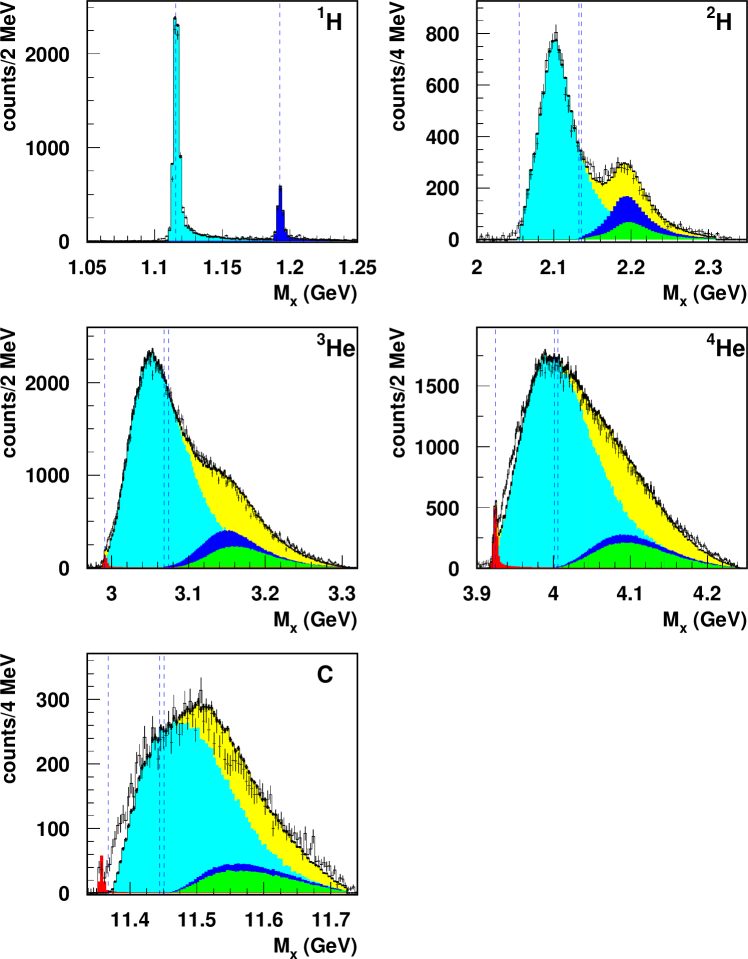
Figure 6: (Color Online) Reconstructed missing mass spectra for six targets at one kinematic setting ($\langle 1.7^{{{}^{\circ}}}\rangle$). The lowest lying thresholds for quasifree production of $\Lambda$ and $\Sigma$ hyperons on each targets are indicated by the dot-dashed vertical lines. For hydrogen, these lines correspond to the pole masses of the $\Lambda$ and $\Sigma^{0}$ hyperons, respectively. Simulated quasifree reactions A$(e,e^{\prime}K^{+})$Y are indicated by colors: $Y=\Lambda$ (lightblue), $Y=\Sigma^{0}$ (blue), $Y=\Sigma^{-}$ (green), bound states ${}^{3}_{\Lambda}$H, ${}^{4}_{\Lambda}$H, ${}^{12}_{\Lambda}$B (red), sum of all simulated contributions (yellow).

Figure 7: Comparison of the nuclear cross section for quasifree $\Lambda$, $\Sigma^{0}$ and $\Sigma^{-}$ production on ³He targets. For comparison, the respective quasifree distribution on the proton are shown by open symbols. These points have been scaled by a factor of 2 for better comparison.

Figure 8: Comparison of the nuclear cross section for quasifree $\Lambda$, $\Sigma^{0}$ and $\Sigma^{-}$ production on ⁴He targets. The respective quasifree distributions on the proton are shown by open symbols. These points have been scaled by a factor of 2 for better comparison.