A formally exact field theory for classical systems at equilibrium.

Abstract

We propose a formally exact statistical field theory for describing classical fluids with ingredients similar to those introduced in quantum field theory. We consider the following essential and related problems : $i$) how to find the correct field functional (Hamiltonian) which determines the partition function, $ii$) how to introduce in a field theory the equivalent of the indiscernibility of particles, $iii$) how to test the validity of this approach. We can use a simple Hamiltonian in which a local functional transposes, in terms of fields, the equivalent of the indiscernibility of particles. The diagrammatic expansion and the renormalization of this term is presented. This corresponds to a non standard problem in Feynman expansion and requires a careful investigation. Then a non-local term associated with an interaction pair potential is introduced in the Hamiltonian. It has been shown that there exists a mapping between this approach and the standard statistical mechanics given in terms of Mayer function expansion. We show on three properties (the chemical potential, the so-called contact theorem and the interfacial properties) that in the field theory the correlations are shifted on non usual quantities. Some perspectives of the theory are given.

I Introduction

In various domains of physics a description in terms of fields is frequently used. Hydrodynamics represents a first example in which some fields (densities, velocities, …) are introduced for describing the properties of a coarse grained entity – the so-called fluid particle. Later, field theory (FT) has been used as a simple and intuitive tool to predict the behaviour of complex systems in the domain of soft matter physics Safran1 ; Pincus1 ; DesCloiseaux ; Gompper ; deGennes . These FT are essentially phenomenological and rely on Hamiltonian functionals introduced in an ad hoc manner. They focus on a mesoscopic scale description and they are based on a more or less explicit coarse graining procedure. In this context, Hamiltonians are introduced to describe large classes of phenomena having similar properties though different in their microscopic details. This further suggests another type of problems where a FT is extensively used i.e. the description of critical phenomena. Here also the FT is based on the assumption that a detailed microscopic knowledge of the system is not relevant to describe its universality class Kadanoff ; ZinnJustin ; Amit ; Ma . And well suited approximations to describe systems with long range correlations or interactions are introduced. In relation, field theory is also used to describe systems with the long ranged Coulomb interactions. In this case, FT is constructed using the Hubbard-Stratonovich transform of the standard partition function KSSHE1 ; KSSHE3 ; Parisi . Better known as the sine-Gordon transform in the case of the Coulomb potential, it has given rise to considerable literature Nabutovskii2 ; Kholodenko3 ; Netz2 ; Netz3 ; Coalson1 ; Caillol2 ; Brilliantov ; Brydges ; Yukh1 . These approaches give an exact description of the systems properties on a microscopic level. In this respect, they are distinct from the soft matter like descriptions based on a coarse graining procedure. The sine-Gordon approaches introduce an auxiliary field and intricate couplings between fluctuating fields. In our opinion, this auxiliary field is essentially a mathematical tool, difficult to associate with any physical quantity. As a result finding meaningful approximations is rather counterintuitive and the application of such approaches requires that one be rather cautious Fisher .
In contrast to these approaches, our main goal is to show that it is possible to write a FT directly in terms of fields using methods similar to those used in quantum field theory (QFT). Namely, we show that it is possible to build the theory around a field, which is a real quantity having a simple physical meaning. Moreover we will show that our FT construction is not only simple and intuitive but also leads to a complete description at microscopic level. In this paper, we consider systems at equilibrium.
The paper is organized as follows. In the next Section we present the main requirements which a FT must verify. In Section III, we give the Hamiltonian on which the FT is based : it contains two terms of different nature. This leads to investigate the Feynman expansion of a purely local Hamiltonian with an infinite number of coupling constants. This is developed in Section IV where some important specific aspects of the expansion are shown. In Section V we calculate the partition function in the presence of an interaction pair potential. In the next Section we establish an exact mapping between our FT and the standard statistical mechanics given in terms of Mayer expansion Balescu . In Section VII we illustrate on several examples how our approach may lead to new aspects in statistical physics. Finally, in Section VIII we give some conclusions and perspectives.

II Requirements for a field theory

Our main assumption is that the partition function $\Xi[\phi]$ of a classical system can be described exactly via a functional integral defined according to

$$\Xi[\phi]=\int\mathcal{D}\phi\exp\left\{-\beta H[\phi]\right\}$$ (1)

in which $\phi$ is a field, $H[\phi]$ a functional of this field which we call Hamiltonian and $\beta=1/(k_{B}T)$ is the inverse of the temperature.
To use (1) we must solve several problems. We have to define $\phi$ and also find an explicit form for $H[\phi]$. It is intuitive to choose for $\phi$ a real quantity as the density of matter $\rho$ for instance. This choice represents a fundamental difference from the Hubbard-Stratonovitch type approaches in which two fields are used, one being a complex quantity. In comparison with the standard description of the liquid state, where the configuration space spans all possible distributions of the particles, here $\rho$ is a function defined everywhere in space. As a consequence the number of degrees of freedom in (1) is related to the space discretization required to calculate the functional integral as opposed to the number of particles. Then we have to solve a new problem, of how to transpose in FT a property mimicking the indiscernibility of particles. To relate the FT and the usual physics we assume that the average of the field, $<\rho>$, corresponds to the actual density of particles noted $\tilde{\rho}$ .

In addition to the indiscernibility of particles, the so-called classical statistical mechanics contains the volume of the elementary cell $\Delta p\Delta x=\hbar$ or, at least, after integration over momenta in the case of systems of at equilibrium, the thermal de Broglie wavelength $\Lambda$. Thus we also have to find how such quantities associated with particles appear in a FT.

In contrast to the Hubbard-Stratonovitch type descriptions which are finite as they represent a rigorous mathematical transformation of a finite quantity, we expect that a field theory, as is often the case, will contain infinities associated with the short scale spatial discretization of the functional integral. This will require the introduction of a renormalization procedure.

Finally, to be able to assert that the FT is also an exact representation, we have to show that there exists a rigorous mapping between the FT and the standard statistical mechanics of dense systems. Hereafter we turn our attention to all these questions.

III Defining the Hamiltonian

To build $H[\rho]$ we follow an approach inspired by the methods developped in QFT where instead of $H[\rho]$ the lagrangian $L[\phi]$ is considered. To find the latter, we select a functional and check that the mean field approximation of the theory reproduces a well known result; for instance, the Maxwell equations in quantum electrodynamics. In this case, $L[\phi]$ can be considered a good choice for elaborating the complete theory including the fluctuations via the functional integral.

In statistical thermodynamics, it is only for systems without interactions, ideal systems, that we know an exact and general result and have the explicit expression of the partition function, $\tilde{\Xi}_{0}$. We then consider such systems and require that the Hamiltonian $H_{0}[\rho]$ reproduce the thermodynamic partition function $\tilde{\Xi}_{0}$ in a mean field estimation of (1). However, since $\tilde{\Xi}_{0}$ is a cornerstone in classical statistical mechanics and contains fundamental physics related to $\Lambda$ and the indiscernibility of particles, we further require that $H_{0}[\rho]$ reproduce $\tilde{\Xi}_{0}$ exactly, i.e. also beyond the mean field approximation. These fundamental aspects will then be correctly accounted for in the FT for all systems including those with interactions. We shall now discuss the Hamiltonian.

Having chosen the field $\rho$ so that its average corresponds to the density of particles $\tilde{\rho}$, it is evident to fix the chemical potential, $\mu$, and choose for $\tilde{\Xi}_{0}$ the grand canonical partition function. In this case we have the exact thermodynamic results

$$\ln\tilde{\Xi}_{0}=\beta pV=\tilde{\rho}V$$ (2)

and

$$\beta\mu=\ln(\tilde{\rho}\Lambda^{3})$$ (3)

where the exact density $\tilde{\rho}$ is uniformly distributed in space. A simple Hamiltonian $H_{0}[\rho]$ that reproduces (3) in a mean field approximation of (1) is

$$\beta H_{0}[\rho]=\int d\mathbf{r}\left\{\rho(\mathbf{r})\left[\ln\left(\rho(\mathbf{r})\Lambda^{3}\right)-1\right]-\beta\mu\rho(\mathbf{r})\right\}.$$ (4)

As for the lagrangian $L[\phi]$ in QFT we cannot claim that $H_{0}[\rho]$ is unique. However we see that the part

$$F[\rho]=\int d\mathbf{r}\;\rho({\mathbf{r}})\left[\ln\left(\rho({\mathbf{r}})\Lambda^{3}\right)-1\right]$$ (5)

of $H_{0}[\rho]$ represents, in the mean field approximation, the free energy of an ideal system i.e. the kinetic energy and the entropy. In Section VII, we compare $F[\rho]$ with the DFT (density functional theory) DFT1 ; DFT2 ; DFT3 where a similar term appears.

The requirement that $H_{0}[\rho]$ gives the exact result entails a more careful analysis of the functional integral $\Xi_{0}[\rho]$. In order to calculate practically (1), we have to introduce in the r.h.s. a lattice with a spacing $a$. The result will then depend on this parameter. In the following, our intention is to find the conditions to obtain the exact thermodynamic result whatever the value of $a$. The discrete form of $\beta H_{0}[\rho]$ is

$$\beta H_{0}[\rho] = \sum_{i}^{V/a^{3}}\rho({\mathbf{r}_{i}})a^{3}\left[\ln\left(\rho({\mathbf{r}_{i}})\Lambda^{3}\right)-1\right]-\beta\mu\sum_{i}^{V/a^{3}}\rho(\mathbf{r}_{i})a^{3}$$ (6)

and the partition function becomes

$$\Xi_{0}[\rho] = \int\prod_{i=1}^{V/a^{3}}d[\rho(\mathbf{r}_{i})a^{3}]\;e^{-\beta H_{0}[\rho]}$$ (7)

where we have used in the measure the dimensionless quantity $\rho(\mathbf{r}_{i})a^{3}$. Due to the local character of $H_{0}[\rho]$, the calculation of $\Xi_{0}$ is a product of usual integrals, such as

$$\int d[\rho(\mathbf{r}_{i})a^{3}]\exp\left\{-\rho({\mathbf{r}_{i}})a^{3}\left[\ln\left(\rho({\mathbf{r}_{i}})\Lambda^{3}\right)-1\right]+\beta\mu\rho(\mathbf{r}_{i})a^{3}\right\}.$$ (8)

Beyond the saddle point, we have

$$\ln\Xi_{0}[\rho]=\tilde{\rho}V\left[1+\frac{1}{\tilde{\rho}a^{3}}\psi[\tilde{\rho}a^{3}]\right]$$ (9)

where the function $\psi$ given in A represents the correction to the exact thermodynamic result $\tilde{\rho}V$ given in (2). As expected, the correcting term becomes negligible when $\tilde{\rho}a^{3}$ is large. However, the discretization has introduced a cumbersome dependence on the lattice spacing $a$, which we would like to dispose of keeping only physically meaningful terms. Before discussing this point, we generalize this result for an external potential.

Having to calculate local integrals the previous result for the partition function can be easily extended by changing $\beta\mu$ into $\beta\mu-V^{ext}(\mathbf{r}_{i})$ where the external potential is in temperature reduced units. Instead of (9) we now have

$$\ln\Xi_{0}[\rho,V^{ext}]=\sum_{i}^{V/a^{3}}{\tilde{\rho}}a^{3}e^{-V^{ext}(\mathbf{r}_{i})}+\sum_{i}^{V/a^{3}}\psi[{\tilde{\rho}}a^{3}e^{-V^{ext}(\mathbf{r}_{i})}]$$ (10)

where the last term in the r.h.s. of (10) is given in A. If $V^{ext}(\mathbf{r}_{i})\approx 1$, the corrective term is still negligeable when ${\tilde{\rho}}a^{3}$ is large. Equation (10) is correct as long as $V^{ext}(\mathbf{r}_{i})$ does not vary rapidly on the distance $a$ which is already large in comparison with the mean distance between particles ($\approx\tilde{\rho}^{-1/3}$). This condition is a restriction on the validity of (10).
It is possible to release such constraint and generalize eq. (10) to any external potential by noticing that all physical terms for this system have a well defined dependence on the lattice spacing, distinct from the corrections associated with $\psi$. We now take into account the following quantity

$$\ln\Xi_{0}^{R}[\rho,V^{ext}] = \ln\Xi_{0}[V^{ext}]-\sum_{i}^{V/a^{3}}\psi[{\tilde{\rho}}a^{3}e^{-V^{ext}(\mathbf{r}_{i})}]$$ (11)

$$= \sum_{i}^{V/a^{3}}{\tilde{\rho}}a^{3}e^{-V^{ext}(\mathbf{r}_{i})}.$$ (12)

The renormalized quantity is now equal to its value at the saddle point whatever the value of $a$. From an operational point of view this result must be understood as follows : $\exp\{-\beta H_{0}[\rho]\}$ is a formal expression. It represents an expansion of the exponential around its saddle point value and in this expansion terms corresponding to $\psi[\tilde{\rho}a^{3}e^{-V^{ext}(\mathbf{r}_{i})}]$ are discarded in order to obtain the physical quantities.

In the limit $a\rightarrow 0$, the renormalized grand potential is now a finite quantity and its value

$$\ln\Xi_{0}^{R}[\rho,V^{ext}]=\int{\tilde{\rho}}\,e^{-V^{ext}(\mathbf{r})}d\mathbf{r},$$ (13)

corresponds to the standard statistical mechanics result valid for any external potential which is independent from $a$.
Note that the change of limit due to the presence of a potential is a standard problem in statistical mechanics as shown in Hill . For an ideal system the so called classical statistical mechanics is obtained in the limit $\hbar\to{0}$ whatever the value of $\Lambda$. However, in the presence of an interaction potential, an extra limit $\Lambda\to{0}$ must be taken in order to keep all information about the interaction potential.

From the results obtained in this Section we assume that the total Hamiltonian will be in the form of

$$\beta H[\rho]=\beta H_{0}[\rho]+\frac{1}{2}\int d\mathbf{r}d\mathbf{r}^{\prime}\rho({\mathbf{r}})\beta v(\mathbf{r}-\mathbf{r^{\prime}})\rho({\mathbf{r^{\prime}}})$$ (14)

where at this stage there is a non-local term due to the presence of the interaction pair potential $v(\mathbf{r}-\mathbf{r^{\prime}})$.

Hereafter our main goal is to give an operational meaning to (14) as we have already done in the case of $\beta H_{0}[\rho]$. To calculate the partition function, we need to expand $\exp\{-\beta H[\rho]\}$. In QFT the calculation of similar quantities is done by introducing a gaussian propagator and performing the so-called loop expansion. Here $H_{0}[\rho]$ is purely local and it is not traditional to give a Feynman expansion for such a term. We have to find a formal propagator and a loop expansion associated with $H_{0}[\rho]$ in order to be able to treat the local and non local part of $H[\rho]$ on the same footing. In the next Section we shall investigate the properties of $H_{0}[\rho]$ and will show that this expansion is also fundamental when an interaction potential is present.

IV Feynman expansion of $H_{0}[\rho]$.

By using the fact that $H_{0}[\rho]$ is local we have obtained a first expansion eqs. (10) and (50) of $\Xi_{0}[V^{ext}]$. In parallel a second expansion can be performed with Feynman graphs. Since both expansions are expressed in terms of ${\tilde{\rho}}a^{3}$ and $-V^{ext}$ we may identify term by term the expansion coefficients and by this method, as we shall see, solve complex problems of combinatory.
To have a simple Feynman expansion, we choose a constant field $\rho_{z}$ as a reference state. Our choice - obviously not unique - is to take ${\rho}_{z}=e^{\beta\mu}/\Lambda^{3}$ corresponding to the activity hansenbook . This choice combines two interesting points : $i$) it gives an expansion in terms of activity which will be useful when comparing in Section VI our results to the Mayer expansion and $ii$) it leads to a very simple propagator.

IV.1 Gaussian propagator, perturbative expansion.

Hereafter we write the field as $\rho(\mathbf{r})={\rho}_{z}+\delta\rho(\mathbf{r})$ and we have

$$\beta{H}_{0}[\rho,V^{ext}] = \beta{H}^{(0)}_{0}[{\rho}_{z},V^{ext}]+\beta{H}^{(2)}_{0}[\delta\rho]+\beta\delta{H}[\delta\rho,V^{ext}]$$ (15)

where the first term is constant

$$\beta{H}^{(0)}_{0}[{\rho}_{z},V^{ext}]=-{\rho}_{z}V+\sum_{i}^{V/a^{3}}V^{ext}(\mathbf{r}_{i}){\rho}_{z}a^{3}.$$ (16)

The second term is quadratic

$$\beta{H}^{(2)}_{0}=\frac{1}{2{\rho}_{z}a^{3}}\sum_{i,j}^{V/a^{3}}\delta\rho({\mathbf{r}_{i}})a^{3}\;\delta_{ij}\;\delta\rho({\mathbf{r}_{j}})a^{3}$$ (17)

and the Kronecker $\delta_{ij}$ plays formally the role of an interaction. Following the terminology of the QFT we call the quadratic term propagator. The remaining term represents the coupling part of the Hamiltonian given by

$$\beta\delta{H}[\delta\rho,V^{ext}] = \sum_{i}^{V/a^{3}}V^{ext}(\mathbf{r}_{i})\delta\rho({\mathbf{r}_{i}})a^{3}+\sum_{i}^{V/a^{3}}\sum_{l\geq 3}^{\infty}\frac{(-1)^{l}(l-2)!}{({\rho}_{z}a^{3})^{(l-1)}}\left(\frac{1}{l!}[\delta\rho(\mathbf{r}_{i})a^{3}]^{l}\right).$$ (18)

It shows the specificity of the present FT, with an infinity of coupling terms whose coefficients depend on a numerical factor and the parameter ${\rho}_{z}a^{3}$.
In order to achieve a diagrammatic expansion we rewrite the partition function according to

$$\Xi_{0}[V^{ext},J] = \int\prod_{i=1}^{V/a^{3}}d[\rho(\mathbf{r}_{i})a^{3}]\;\exp\left\{-\frac{\beta{H}_{0}[\rho,V^{ext}]}{\alpha}+\sum_{i}^{V/a^{3}}J(\mathbf{r}_{i})\rho({\mathbf{r}_{i}})a^{3}\right\}$$ (19)

where ${H}_{0}[\rho,V^{ext}]$ includes the external potential, $J$ is a generating field and $\alpha$ is a parameter, formally equal to $1$, which is useful to organize the loop expansion in QFT ZinnJustin ; Amit . We can perform the functional integral, using the gaussian integrals Kadanoff ; ZinnJustin ; Amit ; Ma and express the result formally as

$$\Xi_{0}[V^{ext},J]=\exp\left\{-\frac{\beta{H}^{(0)}_{0}[{\rho}_{z},V^{ext}]}{\alpha}\right\}\left(\sqrt{2\pi{\rho}_{z}a^{3}\alpha}\right)^{V/a^{3}}$$

$$\exp\left\{-\frac{\beta}{\alpha}\delta{H}\left[\frac{\delta}{\delta J},V^{ext}\right]\right\}\exp\left\{\frac{\alpha{\rho}_{z}a^{3}}{2}\sum_{i,j}^{V/a^{3}}J(\mathbf{r}_{i})\delta_{ij}J(\mathbf{r}_{j})\right\}.$$ (20)

The second line introduces the operator obtained by replacing the field $\delta\rho(\mathbf{r})a^{3}$ with the derivation operator $\delta/\delta J(\mathbf{r})$

$$\beta\delta{H}\left[\frac{\delta}{\delta J},V^{ext}\right] = \sum_{i}^{V/a^{3}}V^{ext}(\mathbf{r}_{i})\frac{\delta}{\delta J(\mathbf{r}_{i})}+\sum_{i}^{V/a^{3}}\sum_{l\geq 3}^{\infty}\frac{(-1)^{l}(l-2)!}{({\rho}_{z}a^{3})^{(l-1)}}\left(\frac{1}{l!}\left[\frac{\delta}{\delta J(\mathbf{r}_{i})}\right]^{l}\right).$$ (21)

This operator is applied to the last term in the r.h.s. of (IV.1) which is gaussian Kadanoff ; ZinnJustin ; Amit ; Ma . The calculation is performed expanding the operator $\exp\left\{-(\beta/\alpha)\delta{H}\left[\delta/\delta J,V^{ext}\right]\right\}$. Taking $J=0$ at the end of the calculation, we select terms with pairs of derivatives acting on the same quadratic form, which corresponds to the well known Wick theorem Kadanoff ; ZinnJustin ; Amit ; Ma . Note that going from the density field representation of $\Xi_{0}$ to the generating functional representation, we invert the kernel of the quadratic form. In the present case, this is a simple operation which consists in taking the inverse coefficient.

IV.2 Diagrammatic representation

The diagrammatic representation of the theory is organized Kadanoff ; ZinnJustin ; Amit ; Ma around vertices representing couplings of the field obtained from the expansion of $\exp\{-\beta\delta{H}/\alpha\}$ and lines joining the vertices representing the propagator. The symbols used to draw these elements are shown in figure 1.

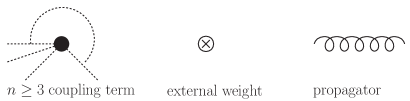
Figure 1: Diagrammatic elements for the graph representation.

The propagator is represented by a curly line. The coupling terms will be denoted by a black circle, where three or more propagators can be joined, the precise number is understood from the number $n$ of lines joined to it. An important feature in knowing explicitly the Hamiltonian functional is that, as opposed to the phenomenological FT, we can workout precisely all coefficients for the couplings. Hence, besides the standard $1/n!$, the coefficient is $(-1)^{(n-1)}(n-2)!/({\rho}_{z}a^{3})^{n-1}$. The case of the vertex, with only one line attached to it, is drawn by a crossed circle and is associated with the external weight $-V^{ext}(\mathbf{r})$. Depending on whether we use the generating functional representation or not, a coupling term may represent $[\delta\rho(\mathbf{r})a^{3}]^{n}$ or $\left[\delta/\delta J(\mathbf{r})\right]^{n}$. Furthermore, otherwise specified, we shall take into account connected graphs related to the logarithm of the partition function.

Let us now define some topological elements. The external branches are the one body coupling constants together with the only propagator which can be attached to it. Internal lines are propagators which are not in external branches.

The graph in figure 2 is an example of a diagram.

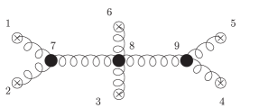
Figure 2: Example of a diagram.

The points $7$, $8$, $9$ are vertices, the points $1,...,6$ are the external weights and there are $6$ external branches and two internal lines.

IV.3 Topology.

IV.3.1 Dimensional analysis.

The diagrammatic representation of $\ln\Xi_{0}[\rho]$ leads to an infinity of graphs that we can classify, as common practice in FT, by using a dimensional analysis in terms of the parameter $\alpha$ Kadanoff ; ZinnJustin ; Amit ; Ma . This corresponds to the loop expansion. A diagram with $L$ loops is dimensionally associated with $\alpha^{L-1}$. For instance, the diagram in Figure 2, which is a tree diagram ($L=0$), is indeed proportional to $1/\alpha$. In the following, our purpose is to show that the dimensional analysis in terms of the formal parameter $\alpha$ can be associated with a physical parameter of the system.
The standard analysis allows to relating the number of elements in a graph (lines, vertices) to the number of loops Kadanoff ; ZinnJustin ; Amit ; Ma according to

$$L-1=I+E-m$$ (22)

where $I$ is the number of internal lines, $E$ the number of external lines, and $m$ the number of vertices. These include also the one point vertices. The latter associated with the external potential set the power in $-V^{ext}$. The r.h.s. of this relation shows that the power in $\alpha$ of the graph corresponds, in agreement with the expression of the partition function eq. (IV.1), to a factor $1/\alpha$ for each of the $m$ vertices, $\alpha^{(I+E)}$ for the internal and external lines. It is tempting to consider the quantity ${\rho}_{z}a^{3}$ instead of $\alpha$ which appears in the calculation in a similar way. Here, we also have to account for the power of this term in each coupling term, eq. (18). Let $m_{i}$ be this power for each of the $m$ coupling vertices. Considering that each line is attached to two vertices, we have

$$\sum_{i=1}^{m}m_{i}=2I+2E.$$ (23)

Using eq. (22)

$$\sum_{i=1}^{m}m_{i}=2(L+m-1)$$ (24)

which is also

$$-\sum_{i=1}^{m}(m_{i}-1)+I+E=-(L-1)$$ (25)

On the left hand side we recognize the contribution in powers of ${\rho}_{z}a^{3}$ in the graph : each vertex contributes $1/({\rho}_{z}a^{3})^{m_{i}-1}$, and there are $I+E$ lines each contributing ${\rho}_{z}a^{3}$. Thus we obtain a relation between the overall power of ${\rho}_{z}a^{3}$ of the graph and the number of loops. The role of the parameter for ${\rho}_{z}a^{3}$ is then equivalent to that of $1/\alpha$. In the following, we no longer introduce the factor $\alpha$, as its role is redundant. All graphs can be computed exactly and we shall avoid explicit indexing of the points in the expressions, as finally all points are the same and we shall only discuss combinatory. The value of a graph is a numerical coefficient, a power of ${\rho}_{z}a^{3}$ and of $-V^{ext}(\mathbf{r})$.

IV.3.2 Tree graphs.

First we take the case $L=0$, which corresponds to tree graphs. From dimensional analysis, all tree graphs with $n$ external branches are proportional to ${\rho}_{z}a^{3}[-V^{ext}(\mathbf{r}_{i})]^{n}$ and the value of their sum can be written as

$${\rho}_{z}a^{3}\;c_{n}\;[-V^{ext}(\mathbf{r}_{i})]^{n}$$ (26)

where $c_{n}$ is a combinatorial coefficient. The value can be obtained by equating this expression, linear in ${\rho}_{z}a^{3}$ with the corresponding term in eq. (11) for each point $\mathbf{r}_{i}$. Thus

$${\rho}_{z}a^{3}\left(\sum_{n=0}^{\infty}c_{n}[-V^{ext}(\mathbf{r}_{i})]^{n}\right)={\rho}_{z}a^{3}e^{-V^{ext}(\mathbf{r}_{i})}.$$ (27)

Order by order in powers of $V^{ext}$, this equation sets $c_{n}=1/n!$ for any $n\geq 3$ and we can generalize the notion of trees to all $n$. Indeed, one can verify that the cases $n=0$ and $n=1$ relate to the expression of $\exp\left\{-\beta H[{\rho}_{z}a^{3}]\right\}$ in eq. (15) and give $c_{0}=1$ and $c_{1}=1$ moreover the calculation of the quadratic term in $V^{ext}$ gives $c_{2}=1/2$. Now we know the combinatory for the $n$-tree graphs. The result is extremely simple.
Of course $c_{n}$ can be also calculated directly by performing the sum of graphs, such a direct calculation shows that the rather simple and intuitive value of $c_{n}$ results in fact from the combination of different graphs.

IV.3.3 Loop graphs.

Let us now consider the class of connected diagrams which have at least one loop ($L\geq 1$) and $n$ external branches that we refer to as $n^{L}$-loop graphs.

For $L>1$, the dimensional analysis states that a given $L$ corresponds to a power of $1/({\rho}_{z}a^{3})$. We consider graphs with $L>1$ loops and $n$ external branches. For given values of $L$ and $n$, the dimensional analysis for the sum of all such graphs leads to the expression

$$\frac{d_{L}}{(\rho_{z}a^{3})^{(L-1)}}\frac{c^{\prime}_{n,L}}{n!}[-V^{ext}(\mathbf{r}_{i})]^{n}$$ (28)

where $d_{L}$ are the coefficients of the expansion of $\psi$ given in A, and $c^{\prime}_{n,L}$ is a combinatory coefficient.
The case $L=1$ is specific, for $n=0$ we have

$$\frac{1}{2}\ln(2\pi{\rho}_{z}a^{3})$$ (29)

and for $n\geq 1$

$$\frac{c^{\prime}_{n,1}}{n!}[-V^{ext}(\mathbf{r}_{i})]^{n}.$$ (30)

The contributions for any $n$ in eq. (28) - (30) can be obtained from term by term identification with the function $\psi$ in eq. (50) for all powers of ${\rho}_{z}a^{3}$ and $-V^{ext}$. For $L=1$, the comparison gives $c^{\prime}_{1,1}=1/2$ and for $n\neq 1$ and $c^{\prime}_{n,1}=0$. For $L>1$, we must have $c^{\prime}_{n,L}=(1-L)^{n}$. Clearly, the $c^{\prime}_{n,L}$ can be also calculated by performing the sum of the corresponding graphs.

IV.4 Ideal system vertex functions.

In the following, we define an important object in the diagrammatic expansion. For $n\neq 2$, we define the $n^{T}$-vertex functions as the functions obtained from $n$-tree graphs by erasing the $n$ external branches . The value of the sum of all graphs contributing to a $n^{T}$-vertex function is

$${\rho}_{z}a^{3}\frac{1}{n!}\left[\frac{1}{({\rho}_{z}a^{3})}\frac{\delta}{\delta J(\mathbf{r})}\right]^{n}$$ (31)

where $1/({\rho}_{z}a^{3})^{n}$ derives from the fact that we have erased from the tree graph $n$ external propagators and $\left[\delta/\delta J(\mathbf{r})\right]^{n}$ refers to the $n$ points where this vertex function can be combined to the rest of the graph. The combinatorial coefficient is that of the corresponding $n$-tree graph. The generalisation for the case $n=2$ will be given later. The general expression is applicable in this case also. The expression of these tree vertices constitutes an important result of this paper. It states that despite the variety of graphs contributing to an $n^{T}$-vertex, all occurs as if we have a standard coupling of the field at a given point, with a coefficient which besides the standard $1/n!$, is simply 1.

Starting from graphs with any number $n$ of external branches and loops $L$, we define the $n^{L}$-vertex functions, obtained similarly to the tree vertex functions, by removing the $n$ external branches. For $L=1$ there is a single non zero term for $n=1$

$$\frac{1}{2}\left[\frac{\delta}{\delta J(\mathbf{r})}\right]$$ (32)

the other terms for $n\neq 1$ are zero. And for a given $L>1$ and $n$, the value is given by

$$(1-L)^{n}\frac{d_{L}}{({\rho}_{z}a^{3})^{L-1}}\frac{1}{n!}\left[\frac{1}{({\rho}_{z}a^{3})}\frac{\delta}{\delta J(\mathbf{r})}\right]^{n}$$ (33)

where the coefficient is that of the $n^{L}$-loop graphs. The term in square brackets is again simply related to the fact that we have removed the $n$ external branches and created the corresponding attaching points.

IV.5 Renormalization.

In the previous analysis, we have associated topological properties of $n$-tree and $n^{L}$-loop graphs to given powers of ${\rho}_{z}a^{3}$ and of $-V^{ext}$. This has been done in order to relate further this topological analysis with the analytic expression of the generating functional eq. (10). The sum of tree graphs corresponds to the first term in this equation, whereas graphs with at least one loop are part of the second term. As mentionned in Section III, expression (10) depends on the lattice spacing whereas the interest of the renormalized partition function eq. (11) is that it has a finite limit independent of $a$ for vanishing lattice spacing.

Here, in order to free ourselves from the lattice spacing and obtain the renormalized partition function, we define the following renormalization procedure which consists in subtracting all graphs with at least one loop. This is equivalent to susbstracting the term corresponding to the function $\psi$ in the analytic expression of the partition function, eq. (10). This procedure gives a meaning to the formal expression $\exp\{-\beta H_{0}[\rho]\}$ by giving an operational description in terms of diagrams. Note that after renormalization, we no longer, strictly speaking, consider $H_{0}$ and thus this functional should not be directly compared with other formalisms where it appears. From this procedure, we now have a diagrammatic expansion of the renormalized partition function which corresponds to the exact result for an ideal system and which can be used for any value of $a$ in particular in the limit of vanishing $a$, which we discuss in the next Section.

In the following, we shall study the system with interactions and show that the same graphs as discussed in this Section appear. We will see that for the reason of locality the renormalization described here can be applied in this context and that we can obtain a well behaved theory also for the system with interactions.
The present discussion may appear like a cumbersome way of treating the simple ideal system. However, the crucial point is to understand how the counting properties for the particles transpose to the FT. In the following, the main tools introduced in this Section will be used to analyse the case of a system with interactions, as we are now able to expand in the same way both local and non local terms in $H[\rho]$ using the Feynman expansion.

V Feynman expansion of the full Hamiltonian

Hereafter we study the generating functional

$$\Xi[J] = \int\prod_{i=1}^{V/a^{3}}d[\rho(\mathbf{r}_{i})a^{3}]\;\exp\left\{-\beta{H}[\rho]+\sum_{i}^{V/a^{3}}J(\mathbf{r}_{i})\rho({\mathbf{r}_{i}})a^{3}\right\}$$ (34)

in which ${H}[\rho]$ is given in (12). Expanding the field around the activity ${\rho}_{z}$, we obtain

$$\beta{H}[\rho] = \beta{H}^{(0)}[{\rho}_{z},V^{ext}]+\beta{H}^{(2)}[\delta\rho]+\beta\delta{H}[\delta\rho,V^{ext}].$$ (35)

The first contribution is

$$\beta{H}^{(0)}[{\rho}_{z},V^{ext}] = -{\rho}_{z}V+\frac{1}{2}{\rho}_{z}V\tilde{v}_{0}+{\rho}_{z}\tilde{V}^{ext}_{0}$$ (36)

where we define $\tilde{v}_{0}=\beta{\rho}_{z}\sum_{j\neq i}^{V/a^{3}}v(r_{ij})a^{3}$ and $\tilde{V}_{0}^{ext}=\sum_{i}^{V/a^{3}}V^{ext}(r_{i})a^{3}$. In the following, we assume that we have substracted the self energy and that the interaction potential cannot be taken at the same point, although to simplify the notation we do not explicitly indicate it. The quadratic Hamiltonian is

$$\beta{H}^{(2)}[\delta\rho]=\frac{1}{2{\rho}_{z}a^{3}}\sum_{i,j}^{V/a^{3}}\delta\rho({\mathbf{r}_{i}})a^{3}\;[\delta_{ij}+\beta{\rho}_{z}a^{3}v({r}_{ij})]\;\delta\rho({\mathbf{r}_{j}})a^{3}$$ (37)

As noted earlier, the Kronecker $\delta_{ij}$ will be treated as an interaction. The coupling Hamiltonian is given by

$$\beta\delta{H}[\delta\rho,V^{ext}] = \sum_{i}^{V/a^{3}}\delta\rho(\mathbf{r}_{i})a^{3}\tilde{v}(\mathbf{r}_{i})+\sum_{i}^{V/a^{3}}V^{ext}(\mathbf{r}_{i})\delta\rho(\mathbf{r}_{i})a^{3}$$ (38)

$$+\sum_{i}^{V/a^{3}}\sum_{l\geq 3}^{\infty}\frac{(-1)^{l}(l-2)!}{({\rho}_{z}a^{3})^{(l-1)}}\left(\frac{1}{l!}[\delta\rho(\mathbf{r}_{i})a^{3}]^{l}\right)$$

where $\tilde{v}(\mathbf{r})=\beta\rho_{z}a^{3}v(\mathbf{r})$. We point out that this coupling Hamiltonian is essentially the same as for $H_{0}[\rho]$ with the exception of a linear term which includes the interaction potential. Therefore the topology of the diagrammatic expansion will be similar to the expansion for $H_{0}[\rho$]. The main modifications are in the existence of a new contribution to the propagator and to the one body term. We then have for the generating functional

$$\Xi[J]=\exp\left\{-\beta{H}^{(0)}[{\rho}_{z};J]\right\}\left(\sqrt{2\pi{\rho}_{z}a^{3}}\right)^{V/a^{3}}$$ (39)

$$\exp\left[-\beta\delta{H}\left[\frac{\delta}{\delta J};J\right]\right]\exp\left\{-\frac{{\rho}_{z}a^{3}}{2}\sum_{i,j}^{V/a^{3}}J(\mathbf{r}_{i})[\delta_{ij}+\tilde{v}({r}_{ij})]^{-1}J(\mathbf{r}_{j})\right\}$$

where, like in Section IV, we have substituted $\delta\rho\,a^{3}$ by the $\delta/\delta J$ and the notation $[\ldots]^{-1}$ indicates the inverse. The latter can be expanded according to

$$[\delta_{ij}+\tilde{v}({r}_{ij})]^{-1}=\delta_{ij}-\tilde{v}({r}_{ij})+\sum_{k}^{V/a^{3}}\tilde{v}({r}_{ik})\tilde{v}({r}_{kj})+\ldots.$$ (40)

In this expression, the Kronecker $\delta_{ij}$ is its own inverse and the rest represents a sum of terms of alternate signs constituted with chains of single potentials. The diagrammatic representation of this equation is given in figure 3, where the full propagator appears on the l.h.s. while on the r.h.s. the curly line is the Kronecker $\delta_{ij}$ and the lines represent a single interaction potential $-\tilde{v}(r_{ij})$.

Figure 3: Diagrammatic representation of the decomposition eq. (40).

We can thus generalize the notion of the tree vertex function of Section IV.4 to the two body coupling term associated with a weight $1/(2{\rho}_{z}a^{3})$. The diagrammatic expansion will be the same as the one given in the previous section, except that the full double line replaces the curly line and that the external weight has two contributions shown in figure 4.

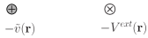
Figure 4: Diagrammatic notation for the weights at the end of the external branches.

V.1 Topological reduction : ideal system vertex functions.

Hereafter we expand the propagator according to the decomposition shown in figure 3. The purpose is to apply a topological resummation of the theory in terms of the vertex functions introduced in Section IV.4. These vertex functions include at least two attaching points. The case of the one body coupling term will be detailed separately.

On the graph given in figure 5, we present an example of this expansion, where the diagram on the right represents a possible decomposition of the total propagator of the original graph on the left. We have omitted the labels and arbitrarily chosen one of the external weights $-V^{ext}$.

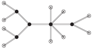
$\Longrightarrow$       

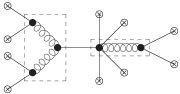
Figure 5: Example of a tree diagram with one possible decomposition.

On the right, for simplicity, we have chosen only the contribution to the chain of interactions corresponding to a single interaction. These aspects are irrelevant to the present discussion. Given the local nature of the ideal system couplings and propagators, it is interesting to isolate in the diagrams the local parts which are indicated inside the dotted frame on the figure. Their contribution to the graph is a numerical coefficient as they are independent on the rest of the graph.

We then consider graphs with the same backbone structure in terms of the interaction potentials but with a different local part like, for instance, in figure 6.

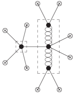
Figure 6: Diagram which has the same structure for the interactions as the diagram in figure 5, but a different topology for the ideal propagator.

The sum of all such local diagrams can be performed using the $n^{T}$-vertex functions as defined in Section IV.4. In the present case, it requires the $5^{T}$-vertex and $7^{T}$-vertex functions derived from the $5^{T}$-tree and $7^{T}$-tree. The resummation into vertex functions is equivalent to a topological reduction. Noting the ideal system vertices introduced in IV.4 by black squares, the graph is now represented by figure 7.

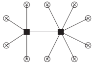
Figure 7: Representation of the sum of all diagrams with the same structure for interactions as the diagram in figure 5 using the $5^{T}$-vertex and $7^{T}$-vertex functions. Amongst these we have the diagrams of figure 5 and figure 6.

Clearly, the new graph corresponds to various topologically different graphs of the original expansion in terms of the total propagator. The factor associated with each ideal system vertex function is simply according to Section IV.4 : $1/[n!({\rho}_{z}a^{3})^{(n-1)}]$.
We hereafter detail the special case of the one body coupling which according to figure 4 can have different weights : the interaction potential or the external potential. $i)$ First we discuss the case when the external branch has a weight $\tilde{v}$. This weight can be attached on the ideal system propagator or on a chain of one or more potentials. These two cases are complementary to allow for any number of interactions in the chain. $ii)$ Then we consider the external branch associated with the external potential. The case when there is a single interaction potential on which we attach the external potential is specific. It is shown in figure 8 where one may verify that all cases with any number of $-V^{ext}$ are represented.

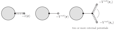
Figure 8: Resummation of external branches with external potential on the one body coupling terms. The gray circle may represent any diagram and the black square a three or higher vertex function.

For the case of a single interaction potential and all other cases, it is straightforward to find that any coupling term can be decorated with a factor $e^{-V^{ext}}$.

The topologigal reduction, presented here on a tree graph using the ideal system tree vertex, can be generalized to graphs which include loops for the ideal system. The separation into non local and local parts related with the ideal propagator can be performed in an identical way. We then also need to introduce the ideal system loop vertices. Having performed the topological reduction of all local parts using either tree vertices or loop vertices, we note that graph with an identical structure may appear once with a tree vertex and once with a loop vertex. For a given position of all other vertices, we can combine the tree vertex and a loop vertex as they are taken at the same point knowing that the rest of the graph is identical. The sum of these two vertices corresponds to the two terms in the ideal system partition function eq. (10). At this stage, we can introduce the renormalization presented in Section IV.5 which corresponds to substracting the loop vertices. As a result we have vertices which are well behaved in the vanishing lattice space limit.

As the potential couples distinct points, note that there cannot be a loop consisting of a single interaction potential. More general loops which may include chains of interaction potential are not concerned by the topological reduction associated with the ideal system and remain unchanged.

V.2 Diagrammatic definition of the partition function.

The result of this Section is that the logarithm of the partition function is given by all possible connected graphs made of non labelled ideal system vertices i.e. $n^{T}$-vertex functions ($n\geq 2$) and internal lines corresponding to a single potential. The coefficients of the vertices are those of the $n^{T}$-vertices given in Section IV.4. The external branches are either the ideal system or a single potential propagator. At the end of the external branches we find the labelled weights shown in figure 4.

VI Mapping between the FT and the Mayer expansion.

In this Section, we show that our field theory is as thorough as the standard methods in statistical physics. In order to do this we compare our expansion with the standard Mayer expansion. To simplify the discussion, we first consider the case where the external potential is zero.

To elaborate this comparison, we take the standard expansion of the grand potential in Mayer functions : $f(\mathbf{r})=\exp[-\beta v(\mathbf{r})]-1$ and activity ${\rho}_{z}$ hansenbook . We further expand the exponential in terms of $-\beta v$ and obtain one and the sum of graphs with $n\geq 1$ lines in parallel representing the potentials multiplied by a factor $1/n!$. This corresponds to an expansion in terms of the single potential introduced in Section V, with all possible connected unlabelled graphs with vertices corresponding to the activity. In the following, this expansion will be referred to as Mayer expansion. The Mayer and Feynman graphs have the same topological elements. They both include all possible connected graphs made of lines and points. To then state the equivalence between the two expansions, we must discuss the following. Firstly, although they have a similar topology, lines and vertices are associated with different quantities. In FT, points are $n^{T}$-vertices and one body external weights, whereas in the statistical mechanics they represent the activity. Secondly, we need to compare the combinatory coefficients for the two expansions. Hereafter, we do not discuss the powers of $a$ as in the final the graph is proportional to $a$ and focus only on ${\rho}_{z}$.

First we discuss the powers in ${\rho}_{z}a^{3}$. From the previous section, Feynman diagrams are based on the $n^{T}$-vertex functions associated with $1/({\rho}_{z}a^{3})^{n-1}$. On these vertices, interaction potential lines are attached which from relation (39) each contribute with $({\rho}_{z}a^{3})^{2}$ (one instance is explicit and one comes from the definition of $\tilde{v}$). This factor can be distributed on the two vertices to which any line is attached. By doing this we associate a single power ${\rho}_{z}a^{3}$ to each vertex and none to the lines. The role of the one body vertex has to be treated separately. In one case, the external weight $\tilde{v}$ is attached to the ideal system propagator. From eq. (37), the only factor ${\rho}_{z}a^{3}$ of the ideal propagator is already distributed to the vertex inside the diagram. One can verify that there remains one factor ${\rho}_{z}a^{3}$ associated with the external weight $\tilde{v}$ and this term corresponds to the activity which should be at the end of an external line in the Mayer expansion. In the second case, the external weight is attached to a single interaction potential. This corresponds to two potentials in series and we can use the two body vertex. We can verify that here also we have the correct number of factors ${\rho}_{z}a^{3}$ once they are redistributed on each vertex and that we retrieve the standard Mayer graph result. The final statement is that although in the Feynman expansion factors ${\rho}_{z}a^{3}$ are associated both with lines and vertices, they can formally be redistributed in order to associate a single instance of this coefficient to each vertex. This corresponds to the Mayer diagrams expansion where the activity is associated to the points.

The second aspect is that the $n^{T}$-vertex functions are associated with the standard $1/n!$ factor. This is exactly the correct combinatory so as to obtain the non labelled graphs of the Mayer expansion, with identical rules for the symmetry of the graphs. One only needs to treat separately the case of the external weight, which includes the interaction potential when it is attached to the ideal propagator. It corresponds in the Mayer expansion to a single potential pending from a graph, the topological equivalent of an external branch in the Feynman expansion. The expected combinatory is found in this case too.

The sum of all these results shows that the Mayer and the Feynman expansion are finally identical. The result can be extended to the system in the presence of an external field, indeed we have shown that any vertex function can be decorated by a factor $e^{-V^{ext}}$. We have seen above that each vertex function can be associated to a factor ${\rho}_{z}a^{3}$, the multiplication of this factor by the exponential corresponds, in the liquid state physics, to the generalization of the activity in the presence of an external field denoted $z^{*}={\rho}_{z}e^{-V^{ext}}$ in hansenbook .

The foremost result of this paper shows that given the renormalization introduced in Section IV.5, the result for the diagrammatic expansion is simple and leads to the equivalence of the Feynman and Mayer graph expansions. We thus fulfil our main objective which is to define a FT capable of describing the system at a microscopic level introducing a simple and intuitive Hamiltonian. This confirms previous results where we have shown that our formalism reproduces two exact results which are the virial theorem virial and the contact theorem ddcjpbjstmolphys2007 which will be discussed in more detail in the next Section. Note that in our formalism, there is no reference to Gibbs ensembles. The difference in number of degrees of freedom associated with the field description and the lattice spacing $a$ calls for the renormalisation which we have introduced in order to reproduce the correct combinatorics for particles.

VII Discussion.

From standard text books Hill ; FeynmanHibbs , we know that the so-called classical statistical mechanics contains two basic properties governed by quantum physics. Namely, the thermal de Broglie wavelength, $\Lambda$, and the indiscernibility of particles which originates from $N$ distinct particles a $N!$ coefficient in the partition function. These elements are not related to the interaction potential. In the present paper, we have shown that a simple local functional together with a renormalization procedure can reproduce these two properties. This procedure is not modified when an interaction pair potential is introduced in the Hamiltonian and consequently we can then demonstrate that the theory is equivalent to the usual statistical mechanics. We have shown that the local functional leads, in perturbation theory, to a simple combinatory of the fields. In each monomial term, the $n$ fields are equivalent and their permutation is associated with the coefficient $1/n!$. In other words, the local functional transposes to the FT the indiscernibility of particles.

One characteristic of our FT is that we have been able to introduce a renormalization procedure through which all the results are finite and independent from, arbitrary lattice spacing, although there exists an infinity of coupling constants. Due to renormalization, the expression $\exp\{-\beta H[\rho]\}$ is formal and we must consider that this quantity is defined by its series expansion around the activity and that some terms in this expansion are cancelled by counter terms; these are independent of the interaction potential, showing that they have no physical meaning but are originated only by a mathematical procedure.

Achieving a microscopically faithful description shows that a simple FT is not necessarily associated with a coarse graining and can have a level of description equivalent to that of the standard statistical mechanics, in contrast to the common conceptions of this type of approach ReissH . Indeed, the measure we have used does not require the introduction of any normalization constant in the partition function, necessary in the case of a coarse grained approach.
We can also compare this FT with other microscopically exact field theoretical descriptions. Considering a field approach without using as a starting point the standard partition function, we deal with a renormalization that does not exist for field theories based on the Hubbard Stratonovich transform. On the other hand, our field is extremely simple and has an obvious physical meaning. This contrasts with the Hubbard Stratonovich type approaches, where we have to work in a complex plane with an auxiliary field for which it is rather difficult to introduce appropriate physical approximations.

We also emphasize that FT is distinct from the DFT. Both approaches are based on the existence of a functional of the density. However, in the two formalisms, the correlations are treated in different ways ReissH ; Evans . In the DFT, the form of the functional includes all correlations and fluctuations and we know that this functional exists but we ignore its exact form. Minimizing this functional yields the equilibrium density distribution. In contrast, in FT the functional is known and simple. The core of the FT formalism is to gradually account for the fluctuations when calculating quantities for the system in a perturbative expansion. One part of $H[\rho]$ is $F[\rho]$ which is formally like the free energy of the ideal system. A similar term $F_{DFT}[<\rho>]$ is introduced in DFT, however it is important to point out the differences between $F[\rho]$ and $F_{DFT}[<\rho>]$. $F[\rho]$ is a functional of a field i.e. a fluctuating quantity where as, at the minimum, $F_{DFT}[<\rho>]$ is a function of the mean value of the fluid density. Moreover, we have mentionned earlier that $\exp\{-\beta H[\rho]\}$ is essentially a formal expression. This illustrates one specificity of the FT : the fluctuations of the ideal term which basically represent the entropy must be considered on the same footing as the fluctuations related to the interaction pair potential.
In this respect, although our FT is equivalent to standard statistical mechanics, the two approaches focus on different aspects of the correlations. This is the case when comparing standard approaches, but the discussion will be extended below for the case of our FT. We are convinced that having at disposal distinct formulations for a given quantity is indeed useful, possibly for acquiring a broader understanding.

VII.1 Examples

Hereafter we illustrate on three examples how FT leads to a new point of view on traditional quantities.

In liquid state theory there are three classical expressions of the chemical potential. One of them corresponds to RowlinsonWidom

$$\ln(\tilde{\rho}(\mathbf{r})\Lambda^{3})+\ln<\exp(\beta u(\mathbf{r}))>+V^{ext}(\mathbf{r}) = \beta\mu.$$ (41)

A second traditional expression is given by RowlinsonWidom ; MoritaHiroike ; StillingerBuff

$$\ln(\tilde{\rho}(\mathbf{r})\Lambda^{3})-c^{(1)}(T,[\rho];\mathbf{r})+V^{ext}(\mathbf{r})=\beta\mu$$ (42)

where $c^{(1)}(T,[\rho];i)$ is the single-particle direct correlation function hansenbook ; MoritaHiroike ; StillingerBuff . Finally, we also have a relation based on a charging process of the interaction potential Hill

$$\ln(\tilde{\rho}(\mathbf{r})\Lambda^{3})+\tilde{\rho}(\mathbf{r})\int_{0}^{1}d\xi\int d\mathbf{r}^{\prime}\beta v(|\mathbf{r}-\mathbf{r}^{\prime}|)g^{(2)}(|\mathbf{r}-\mathbf{r}^{\prime}|;\xi)+V^{ext}(\mathbf{r})=\beta\mu$$ (43)

where $g^{(2)}(r_{ij};\xi)$ is the pair distribution function hansenbook as a function of the charging parameter $\xi$. We note that all these expressions emphasize properties related to the potential, whether calculating the correlations of a quantity involving the interaction, or calculating the single-particle direct correlation function or alternatively considering a charging process of the interaction.

The field theoretical description leads to a new expression which can be obtained by writing that the field is a dummy variable in the functional integral. This leads to the so called Dyson relations FeynmanHibbs ; slovenia and we obtain

$$<\ln(\rho(i)\Lambda^{3})>+\sum_{j;j\neq i}^{V/a^{3}}\beta v(i,j)<\rho(j)>a^{3}+V^{ext}(i) = \beta\mu.$$ (44)

Here the term related to the interactions is rather simple, it expresses the mean potential at a given point without taking into account the correlations. All correlations and fluctuations appear in the calculation of the average of the logarithm of the density field. This contrasts with a simple term like the logarithm of the average density, which appears in standard statistical mechanical expressions or in the DFT. As a consequence, differences in the description and a different organisation of the perturbation expansion in the FT, suggest that one should be able to elaborate new approximations.

Let us consider now the so-called contact theorem which establishes an exact relation between the pressure $p$ existing in a bulk phase and the value of the density profile $\rho(0)$ at the wall enclosing the bulk material. This corresponds to

$$\beta p=\rho(0).$$ (45)

In so far as this relation is concerned, discussing the derivation of this theorem is an opportunity to emphasize the conceptual differences between the various approaches. We mention the kinetic theory of gases, in which this relation is the consequence of the mechanical equilibrium at the interface. In the case of DFT, the derivation is straightforward as we only need to write a displacement of the external potential : the interface, in two different ways. Another derivation JRHenderson is obtained by integrating the BGY equations. In this case, a subtle integration of the correlations through the interface leads to the relation. Within our field theoretical framework, the key element is the local functional which is essential at different levels. It is crucial to obtain the density contact value present in the contact theorem ddcjpbjstmolphys2007 , but it is also necessary to cancel supplementary terms which appear in the demonstration. In this respect, specific relations of the field theory are also required, namely the Dyson type relations slovenia .

Now, in a third example, we illustrate one of the main aspects of the FT, i.e. the existence of an intricate coupling between counting (entropy) and interaction. Let us study the interfacial properties of ionic fluids. From the point of view of the interactions, we know that the important quantity is the charge, the difference of densities of each species. However, this system can also be viewed as a peculiar mixture which has a specific condition due to electroneutrality. From this point of view, we have two terms in the ideal functional describing the indiscernibility for each ion. Thus the natural fields are the densities describing each ion. In ddcjstjpbMolPhys2003a ; ddcjstjpbElectrochimActa , we show, in the specific instance where the natural fields for the ideal and for the interaction term are distinct, that the perturbation theory leads to a coupling of the charge and of the total density field due to the local ideal functional. This has direct consequences.
For the simple neutral interface, we show that there exists a depletion for the quadratic fluctuations of the charge. Then, the entropic coupling between the charge field and the total density field predicts a non trivial profile on the total density ddcjstjpbMolPhys2003a ; ddcjstjpbElectrochimActa . We can verify that the contact value of this total density profile satisfies the exact condition of the contact theorem, for the pressure calculated at the same level of approximation. We have used this phenomenon to analyse the anomalous behaviour of the differential capacitance as a function of the temperature anomalous1 ; anomalous2 which has been thoroughly discussed recently in experiments Tosi1 ; Tosi2 , numerical simulation BodaChan and theoretical approaches MierYTeran ; BodaHolovko ; Sokolowski ; Outhwaite1 . The interest of our analysis is that it provides a simple interpretation and understanding for this phenomenon, associating the decrease in the capacitance with the depletion of the ionic density at the interface at low temperature and providing the physical origin of this depletion.

Moreover, the more detailed account of these entropic effects is fundamental in the case of asymmetric, in valence, electrolytes. In anomalous2 , we have tested our FT by comparing with the results of numerical simulations bodaasym and shown that the theory accounts for all main qualitative properties of the phenomenon, in comparison with other approaches Outhwaite2 which although currently more quantitative fail to take certain features into consideration.

VIII Conclusion

In this paper, we present a field theory describing classical fluids at equilibrium at the same level as the standard statistical mechanics. We introduce a real physical field and construct the Hamiltonian in the spirit of the QFT. This functional includes interactions and a local functional representing the ideal system. The latter characterises our approach and has been thoroughly discussed. In particular, we show that it provides, for the FT, essential ingredients in relation to quantum mechanics. The equivalence of our theory with standard statistical mechanics is shown by establishing that the Feynman expansion of the FT is equivalent to the standard Mayer expansion. The approach is original in that it is not a simple mapping of the standard partition function like other field theories. Consequently, it requires a renormalization which we describe. Its basic interest is that the theory remains simple and intuitive like phenomenological field theories.

Establishing a field theory which is both a simple and exact representation of the statistical mechanics has many advantages. We present possible applications.
Some are related to the FT formalism. We can, for instance, use powerful tools such as discussions in terms of symmetries of the system, of the fields desorption . Also, the fact of having a field variable at the microscopic level should allow for natural bridging with the mesoscopic intuitive approaches which also adopt the field theory description. An example can be found in IonicFT2 where a mesoscopic Hamiltonian is presented.
Another aspect is that this formalism treats fluctuations in a different way. This type of approach would help elaborating small systems, where fluctuations can have the same magnitude as the quantities characterising the system ReissH .
Finally, we have also shown that there is an emphasis on correlations associated with entropic effects. Such emphasis should shed new light on the description of ionic systems, or mixtures. For instance, we believe that the emphasis on the correlations between charge and total density could add to the understanding of criticality in ionic systems. For such systems, the potential couples the charge, whereas criticality characterizes a phenomenon on the total density. Another system of interest in the field of the double layer is the study of asymmetric in charge electrolytes, which exhibit polarization phenomena even in the vicinity of neutral interfaces. As opposed to asymmetric in size ions, this phenomenon is not intuitive. The difference of density of anions and cations for these asymmetric systems seems to be the origin of such phenomena as a consequence again of entropic effects zasymnew .

Appendix A Beyond the ideal system saddle point

Beyond the saddle point, we can compute the integral eq. (8) taking into account the fluctuations of the field, on each lattice site we expand the density field as $\rho=\tilde{\rho}+\delta\rho$, in this case the logarithm of the partition function is

$$\ln\Xi_{0}=\tilde{\rho}V+\frac{V}{a^{3}}\ln\left[\int_{-\infty}^{\infty}dt\,e^{-t^{2}/2}\exp\left(\sum_{n=3}^{\infty}\frac{(-1)^{n+1}t^{n}}{n(n-1)(\tilde{\rho}a^{3})^{n/2-1}}\right)\right]$$ (46)

where $t=(\rho-\tilde{\rho})a^{3}/\sqrt{\tilde{\rho}a^{3}}$. Expanding the last exponent, which makes sense in the limit of large $\tilde{\rho}a^{3}$, we find we have to calculate Gaussian integrals: $\int_{-\infty}^{\infty}t^{2n}e^{-t^{2}/2}dt=\sqrt{2\pi}(2n-1)!!$. The result can be written

$$\ln\Xi_{0}=\tilde{\rho}V+\frac{V}{a^{3}}\psi[\tilde{\rho}a^{3}]=\tilde{\rho}V\left[1+\frac{1}{\tilde{\rho}a^{3}}\psi[\tilde{\rho}a^{3}]\right]$$ (47)

with

$$\psi[\tilde{\rho}a^{3}] = \frac{1}{2}\ln(2\pi\tilde{\rho}a^{3})+\sum_{L=2}^{\infty}\frac{d_{L}}{(\tilde{\rho}a^{3})^{(L-1)}}$$ (48)

$$= \frac{1}{2}\ln(2\pi\tilde{\rho}a^{3})-\frac{1}{24}\frac{1}{(\tilde{\rho}a^{3})}-\frac{1}{48}\frac{1}{(\tilde{\rho}a^{3})^{2}}-\frac{161}{5760}\frac{1}{(\tilde{\rho}a^{3})^{3}}+\ldots$$ (49)

with the exclusion of the first term, $\psi$ is a power series of $1/\tilde{\rho}a^{3}$ which is asymptotically convergent for large $\tilde{\rho}a^{3}$, for which the first values of the coefficients $d_{L}$ are given on the second line.
The expression in the presence of an external potential $V^{ext}(\mathbf{r}_{i})$ is

$$\psi[\tilde{\rho}e^{-V^{ext}(\mathbf{r}_{i})}a^{3}] = \frac{1}{2}\ln(2\pi\tilde{\rho}a^{3})-\frac{1}{2}V^{ext}(\mathbf{r}_{i})+\sum_{L=2}^{\infty}\frac{d_{L}\,e^{-(1-L)V^{ext}(\mathbf{r}_{i})}}{(\tilde{\rho}a^{3})^{(L-1)}}$$ (50)

References

References

- (1) Safran S A 1998 Phys. Rev. Lett. 81 4768; Lukatsky D.B. and Safran S A 1999 Phys. Rev. E 60 5848
- (2) Pincus P and Safran S A 1998 Europhys. Lett. 42 103; Lau A W C, Levine D and Pincus P 2000 Phys. Rev. Lett. 84 4116
- (3) Des Cloizeaux J and Janninck G 1990 Polymers in Solution : their modelling and structure (Oxford : Clarendon Press)
- (4) Gompper G and Schick M 2005 Soft Matter vol. 1 : Polymer Melts and Mixtures (Weinheim : Wiley)
- (5) de Gennes P G 1982 Scaling Concepts in Polymer Physics, (London : Cornell University Press)
- (6) Kadanoff L.P., Baym G. 1962 Quantum statistical mechanics (New York : Benjamin)
- (7) Zinn-Justin J 1989 Quantum Field Theory and Critical Phenomena (Oxford : Clarendon Press)
- (8) Amit D J 1984 Field theory, the renormalization group, and critical phenomena. (Singapore : World Scientific)
- (9) Ma S K 1976 Modern Theory of Critical Phenomena (New York : Benjamin)
- (10) Kac M 1959 Phys. Fluids 2 8; Siegert A J F 1960 Physica 26 S30
- (11) Stratonovich R L 1958 Sov. Phys. Solid State 2 1824; Hubbard J 1954 Phys. Rev. Lett. 3 77 Hubbard J and Shofield P 1972 Phys. Lett. A 40 245
- (12) Parisi G 1988 Statistical Field Theory in Frontiers in Physics (Reading : Addison-Wesley)
- (13) Nabutovskii V M, Nemov N A and Peisakhovic Yu G 1980 Phys. Lett. A 79 98-100
- (14) Kholodenko A L 1989 J. Chem. Phys. 91 4849
- (15) Netz R R 2000 Eur. Phys. J. E 3 131; 2001 5 189; 2001 5 557.
- (16) Netz R R and Orland H 2000 Eur. Phys. J. E 1 203
- (17) Coalson R D and Duncan A 1992 J. Chem. Phys. 97 5653; Coalson R D, Walsh A M, Duncan A and Ben-Tal N 1995 J. Chem. Phys. 102 4584
- (18) Caillol J M and Raimbault J L 2001 J. Stat. Phys. 103 753; Raimbault J L and Caillol J M 2001 J. Stat. Phys. 103 777; Caillol J M 2004 J. Stat. Phys. 115 1461
- (19) Brilliantov N V 1998 Phys. Rev. E 58 2628
- (20) Brydges D C and Martin Ph A 1999 J. Stat. Phys. 96 1163
- (21) Yukhnovskii I R 1990 Physica A 168 999; Yukhnovskii I R 1992 Proc. Steklov Institute Math. 191 223
- (22) Fisher M. 1992 J. Chem. Phys. 96 3352
- (23) Balescu R 1976 Equilibrium and nonequilibrium statistical mechanics (New York : Wiley)
- (24) Hohenberg P and Kohn W 1964 Phys.Rev. B 136, 864; Kohn W and Sham L 1965 Phys.Rev. A 140, 1133
- (25) Lundqvist S and March N H 1983 Theory of inhomogeneous electron gas. (New York : Plenum Press)
- (26) Glushkov A.V., Ivanov L.N. 1992 Phys. Lett. A 170, 33
- (27) Hill T L 1956 Statistical Mechanics (New York : McGraw Hill)
- (28) Hansen J P and McDonald I R 1976 Theory of Simple Liquids (New York : Academic Press)
- (29) Di Caprio D, Stafiej J and Badiali J P in Ionic Soft Matter: Modern Trends in Theory and Applications 2005 Proceedings of the NATO Advanced Res. Workshop Kluwer 206 1
- (30) di Caprio D, Badiali J P and Stafiej J 2007 Mol. Phys. 104 3443
- (31) Feynman R P and Hibbs A R 1965 Quantum Mechanics and Path Integrals (New York : McGraw Hill)
- (32) D. Reguera and H. Reiss 2004 J. Chem. Phys. 120 2558
- (33) R. Evans 1981 Mol. Phys. 42 1169
- (34) Rowlinson J S and Widom B 1982 Molecular Theory of Capillarity. vol. 8 (Oxford : Clarendon Press)
- (35) Morita T and Hiroike K 1961 Prog. Theor. Phys. 25 537
- (36) Stillinger F H and Buff F P 1962 J. Chem. Phys. 37 1
- (37) di Caprio D and Stafiej J 2007 J. Mol. Liq. 131-132 48
- (38) van Swol F and Henderson J R 1986 J. Chem. Soc. Faraday Trans. 2 82 82, 1685
- (39) di Caprio D, Stafiej J and Badiali J P 2003 Mol. Phys. 101 2545, di Caprio D, Stafiej J and Badiali J P 2003 Mol. Phys. 101 3197
- (40) di Caprio D, Stafiej J, Badiali J P 2003 Electrochim. Acta 48 2967
- (41) di Caprio D, Stafiej J and Z. Borkowska 2005 J. Electroanal. Chem. 582 41,
- (42) di Caprio D, Valiskó M, Holovko M and Boda D 2007 Mol. Phys. 104 3777
- (43) Painter K R, Ballone P, Tosi M P, Grout P J and March N H 1983 Surf. Sci. 133 89
- (44) Ballone P, Pastore G, Tosi M P, Painter K R, Grout P J and March N H 1984 Phys. Chem. Liq. 13 269
- (45) Boda D, Henderson D and Chan K Y 1999 J. Chem. Phys. 110 5346; Boda D, Henderson D, Chan K Y, and Wasan D T 1999 Chem. Phys. Lett. 308 473
- (46) Mier-y-Teran L, Boda D, Henderson D and Quinones-Cisneros S E 2001 Mol. Phys. 99 1323
- (47) Holovko M, Kapko V, Henderson D and Boda D 2001 Chem. Phys. Lett. 341 363
- (48) Reszko-Zygmunt J, Sokołowski S, Henderson D and Boda D 2005 J. Chem. Phys. 122 084504
- (49) Bhuiyan L B, Outhwaite C W and Henderson D 2005 J. Chem. Phys. 123 034704
- (50) Valiskó M, Henderson D, and Boda D 2007 J. Mol. Liq. 131-132 179
- (51) Bhuiyan L B, Outhwaite C W and Henderson D 2006 Langmuir 22 10630
- (52) Stafiej J, di Caprio D, Badiali J P 2000 Phys. Rev. E 61 3877
- (53) di Caprio D, Stafiej J and Badiali J P 1998 J. Chem. Phys. 108 8572
- (54) di Caprio D, Valiskó M, Holovko M and Boda D 2008 in preparation