Tracking and vertexing at ATLAS

Abstract

Several algorithms for tracking and for primary and secondary vertex reconstruction have been developed by the ATLAS collaboration following different approaches. This has allowed a thorough cross-check of the performances of the algorithms and of the reconstruction software. The results of the most recent studies on this topic are discussed and compared.

1 Introduction

ATLAS is one of the four experiments at the Large Hadron Collider (LHC) that will produce $pp$ collisions at a centre-of-mass energy of 14 TeV. There will be a bunch crossing every 25 ns, which imposes fast response from the detectors as well as the need to store data from each collision in on-detector pipelines until a decision of the first level of the trigger is taken. Furthermore there will be a very high density of charged tracks: at the nominal luminosity of 10³⁴cm^-2sec^-1 for each bunch crossing there will be about 200 charged tracks and about 15 vertex candidates. The reconstruction of tracks and of primary and secondary vertices at LHC will be a challenging task. The Inner Detector (ID) is the tracking detector of ATLAS and consists of three sub-detectors, whose performances as simulated by the software are extensively described in  IDTDRI ; IDTDRII . The outermost detector is the Transition Radiation Tracker (TRT) consisting of several layers of 4 mm straws in the barrel region (arranged in 3 layers of modules) and 14 Transition Radiation Tracker wheels in the endcap, providing about 30 hits per track and a resolution in the $R\phi$ plane of 170 $\mu m$. The SemiConductor Tracker (SCT) is located in the region between 25 cm to 50 cm in radius and consists of 4 layers of stereo silicon strips detectors in the barrel and 9 disks per side in the endcaps, achieving a resolution of about 17 $\mu m$ and 580 $\mu m$ in the $R\phi$ and $Rz$ plane, respectively. The innermost is the pixel detector  pixel , consisting of 3 layers of silicon pixel detectors (at radius of 5.05, 8.85 and 12.25 cm) in the barrel and 3 disks in each of the endcaps, providing a track resolution of about 11 $\mu m$ in R$\phi$ and 60 $\mu m$ in $Rz$. To reconstruct the tracks, it is essential to take into account the effect of multiple scattering and of the energy loss in the material, which requires a precise knowledge of material in the detector. More complicated tracking algorithms are needed to consider the track resolution degradation at the edges of the ID due to the non-uniformity of the 2T magnetic field provided by the ATLAS solenoid in the ID region.

2 Tracking and vertexing at trigger level

The ATLAS trigger is subdivided into three different trigger selection layers that reduce the 1 GHz interaction rate to 200 Hz.

• The first level trigger (LVL1) is a hardware trigger with a 2.5 ms latency that brings the rate to 75kHz. It uses reduced granularity data of the calorimeter and the muon detectors and identifies geometrical regions of interest (RoI) in the detector.

• The second level of the trigger (LVL2) uses the ID information since it processes in parallel the full information of all sub-detectors in the RoIs defined by LVL1. It has a latency of 10 ms bringing the rate below 2 kHz. Tracking and vertexing can be performed at LVL2.

• Finally the Event Filter (EF) can use algorithms similar to the offline software having a 2s latency time.

The performance of the tracking and vertexing algorithms implemented at ATLAS at LVL2 is described below.

2.1 Tracking at LVL2

The tracking algorithm forms track seeds by fitting with a straight line pairs of space points in the pixel innermost layer (B layer) and in the second logical layer (in a given RoI). The tracks are extrapolated back to the beam line and an Impact Parameter (IP) is obtained for each of them. The track is retained if the IP in the transverse plane with respect to the beam axis is small. The $z$ coordinate of the primary vertex is then obtained as the maximum of the histogram filled with the $z$ intersection of the seeds with the beam line. A third space point is extracted in modules situated in positions where the hits may lay based on the track extrapolation. After having removed the ambiguities due to overlapping space points in triplets using the extrapolation quality, the triplets are fitted and identified with tracks. The efficiency for tracks in jets is 80-90% depending on the luminosity and the event topology and 95% for single electrons.

2.2 $b$-tagging at LVL2

The $b$-jet selection is performed by using the transverse impact parameter $d_{0}$ significance, defined as $S=d_{0}/s(d_{0})$, where $s(d_{0}$) is the error on $d_{0}$ and its dependence on $p_{T}$ is obtained from the simulation.

A secondary vertex algorithm similar to offline but faster is used. The $b$-jet estimator uses a likelihood ratio given by the product of the ratios of the probability densities for each track to come from a $b$-jet or a light-jet,

$$W=\Pi_{i}\frac{f_{b}(S_{i})}{f_{u}(S_{i})}.$$

where $i$ runs over all reconstructed tracks in the jet.

The final discriminative variable is defined as X = W/(1+W). The processing time for $b$-jets is less than 2 ms. The rejection for light quarks is 25% and 15% for a $b$-jet efficiency of 50% and 60% respectively.

3 offline tracking algorithms

Several offline tracking algorithms have been developed at ATLAS: xKalman and iPatRec and only very recently the NewTracking algorithm.

• The xKalman first searches for tracks in the TRT using fast histogramming of straw hits, then it extrapolates back to SCT and pixels and fits the tracks using a Kalman filter that associates clusters to tracks assuming that the noise and all material effects and measurements are Gaussian. Finally, the improved tracks are extrapolated back into the TRT in a narrow region around the extrapolated trajectory, retaining all hits in that region.

• the iPatRec algorithm forms track-candidates in SCT and pixel detectors using space-point combinatorials subject to criteria on maximum curvature and crude vertex region projectivity. A global $\chi^{2}$ fitter is used to fit tracks and associate clusters. Only good tracks are retained for extrapolation in TRT, where TRT hits are added. To limit the contamination from high occupancy, tight cuts are applied on the straw residuals.

• The NewTracking algorithm is mainly a reorganization of the tracking code. At present it is largely based on xKalman, but in the future it will use also tools from iPatRec with the aim of obtaining optimised performances. Furthermore it uses a better detector geometry description.

Table 1 shows the results of a performance comparison done using $t\bar{t}$ events. As can be seen xKalman and iPatRec have comparable performances, slightly better than the newly developed NewTracking, whose performances are going to improve and are already better than the others at the time of writing.

	xKalman	iPatRec	NewTracking
Multiplicity (p¿1 GeV)	16.69	17.06	16.88
Barrel Track eff/fake rate	99%/0.6%	99%/0.7%	96%/2.5%
Transition eff/fake rate	98%/0.6%	98%/0.5%	96%/3.6%
Forward eff/fake rate	98%/0.3%	99%/1.3%	95%/2.7%

Table 1: Performance of the ATLAS offline tracking algorithms obtained using $t\bar{t}$ events. The result of the newly developed NewTracking are very preliminary and already superseeded at the time of writing.

Figures 1 a) and b) show the resolution on the impact parameter in the transverse and longitudinal planes, respectively. A sample of WH events with m_H= 400 $GeV/c^{2}$ has been used for the study, where the W decays to $\mu\nu_{\mu}$ and H to $uu$. Figure 2 shows the momentum resolution versus $p_{T}$ for single muons averaged over all $|\eta|$ and for $\eta$=0.

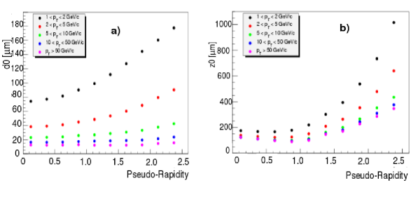
Figure 1: Figure a) and b) show the transverse and longitudinal impact parameter resolution for a sample of WH events with $m_{H}$= 400 $GeV/c^{2}$, where the W is decaying to $\mu\nu_{\mu}$ and the H to $uu$.

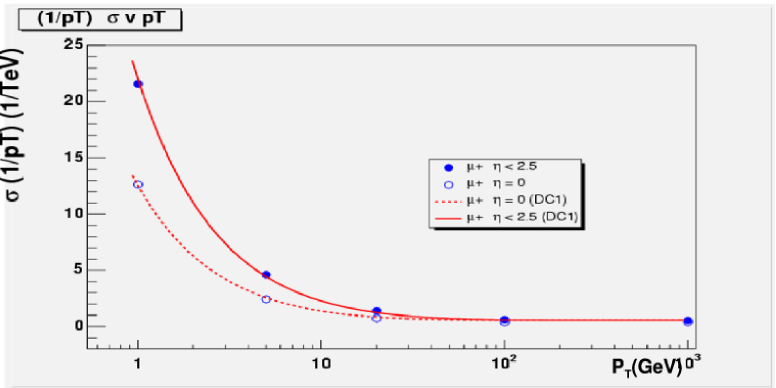
Figure 2: The momentum resolution for single muons versus $p_{T}$ averaged over all $|\eta|$ (full circles) and for $\eta$=0 (open circles). The full lines show results obtained with an older simulation considering only 2 pixel layers instead than 3.

4 Primary vertex reconstruction

Given the large multiplicity of tracks at each bunch crossing (several hundreds as discussed before) the vertex reconstruction must be fast and robust. The input consists of the 3 dimentional trajectories and error matrices of the tracks. Quality requirements on tracks are applied: typically p_T ¿ 1 GeV/c, —d₀— ¡ 0.25 mm, —z₀— ¡ 150 mm and $\chi^{2}$ per track ¡0.5.

The approximate primary vertex position in $z$ is found using a sliding window of 0.7 cm that is moved along the whole interaction region. The window with largest number of tracks, weighted with $p_{T}$ is chosen. The ¡$z$¿ position of the vertex is given by the mean of all the tracks in that window. Tracks belonging to the primary vertex are taken away and the procedure is iterated to get other (pile-up) vertices.

All tracks at $\pm$ 5 mm in $z$ and $\pm$ 1 mm in the transverse plane are accepted as coming from primary vertex. At this point the vertex fitting is performed using a Billoir method. In the fitting procedure the outliers are removed, that is if the $\chi^{2}$ obtained when adding a track is too high, the track is rejected and the fit is recalculated,

There are two different implementations of this method which are basically using the same strategy: VxPrimary and VKalVrt.

A third primary vertex fitter has been developed, the Adaptive Vertex Fitter, that solves the problem of outlier tracks that spoil the fit, not by discarding them, but by down-weighting them. It minimises instead than residuals, the sum of squared residuals weighted with the $\chi^{2}$. Table 2 shows a comparison of the performances of the primary vertex finder algorithms, which give very similar results by following slightly different approaches.

	x($\mu m$)	z($\mu m$)
VxPrimary	12.6 $\pm$ 0.1	50.0 $\pm$ 0.5
AVF	11.07 $\pm$ 0.09	46.76 $\pm$ 0.05
VKalVrt	11.07$\pm$0.09	45.43 $\pm$ 0.05

Table 2: Primary vertex resolution in $x$ and $z$ for the ATLAS primary vertex finders. A sample of simulated WH events with m_H=120 GeV/$c^{2}$ and $W\rightarrow\mu\nu_{\mu}$, $H\rightarrow b\bar{b}$ has been used for the study.

5 ATLAS $b$-tagging

Basic ingredients for the $b$-tagging are the long lifetime of the $b$-hadron jets, the high multiplicity $b$-jets and the impact parameters of the tracks. Additionally the presence of a secondary vertex can increase the rejection power of the $b$ selection. The $b$-tagging algorithms developed by the ATLAS collaboration are based on such properties of the $b$-jet btag . In addition $b$-tagging methods based on the tagging of a soft lepton (electron or muon) resulting from the decay of a $b$-flavoured hadron are being developed.

The standard $b$-tagging identification is based on the 2-dimentional impact parameter of a track in the transverse plane. The method adopted by ATLAS uses the normalised significance $S=d_{0}/s(d_{0})$ for each track and compares it to predefined calibration probability density functions for the $b$ and light quark hypothesis to obtain the probabilities $b(S)$ and $u(S)$. The following discriminating variable (IP2D) for each jet is built by summing over all the tracks in a jet

$$W_{jet}=\sum_{i=1}^{N_{tr}}ln\frac{b(S_{i})}{u(S_{i})}.$$

The discriminative variable consists of logarithms of the density functions ratio, allowing to combine two variables easily. The $b$-tagging performance can be improved by adding the longitudinal and the transverse significance (IP3D):

$$W=\frac{P_{b}(S_{d_{0}},S_{z_{0}})}{P_{u}(S_{d_{0}},S_{z_{0}})}.$$

Figures 3 a) and b) show the distribution of the transverse and longitudinal impact parameter significance for $b$ and light quarks, respectively.

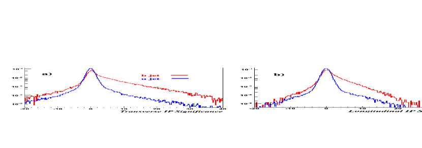
Figure 3: Figure a) and b) show the distribution of the transverse and longitudinal impact parameter significance.

In addition the presence of a secondary vertex is searched for. Only tracks passing the following quality cuts are used: $p_{T}>$ 1 GeV/c, $|\eta|<2.5$, $|d_{0}|<1$ mm, $|z_{0}|<1.5$ mm, number of pixel hits in the B layer greater than 0 and number of pixel hits larger than 1, while more than 6 SCT hits should be detected. The selected tracks are used to search for good 2 track vertices in the jet. At this point vertices that are due to decays of Kaons or Lamdba baryons or to interactions with the beam pipe material, the pixel layers or to photon conversions (V0’s) are removed. A common (inclusive) vertex is formed for the remaining tracks.

Once the secondary vertex is reconstructed some additional discriminating variables can be considered:

1. the number of good two track vertices in the jet,

2. invariant mass of all particles coming from the secondary vertex mass,

3. the ratio of the energy of all particles coming from the secondary vertex and the total energy of the jet.

The variables have been chosen to be independent from tracks impact parameters in order to have a real gain on $b$-tagging performance. The secondary vertex discriminating variable obtained from the probability density functions that parametrize the distributions of these variables can be combined with the track impact parameter based $b$-tagging procedure. Figure 4 a), b and c) show the distribution of the secondary vertex variables for $b$ and light jets.

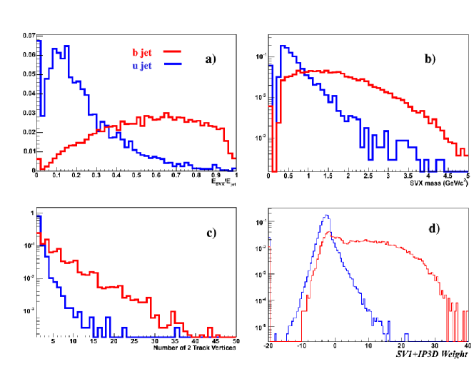
Figure 4: Figure a), b), c) show the distribution of the secondary vertex variables for $b$ and light jets. Figure d) shows the weight obtained by combining SV1 and IP3D.

A jet is labeled as a $b$-jet if there is a $b$-quark within a cone of radius 0.3 around the jet axis, the efficiency for $b$-jets ($\epsilon_{b}$) is defined as the ratio of the number of jets and the number of jets labeled as $b$ with $p_{T}>15$ GeV/c and $|\eta|<2.5$. The light jet rejection is defined as $R_{u}=1/\epsilon_{u}$.

Overlapping jets cause mislabeling and furthermore the jet isolation is very dependent on the type of physics process taken into account. A purification of the jets is done to factorize those effects from pure $b$-tagging issues: light jets are not taken into account if there is a $b$/$c$/quark/hadron within a cone of radius 0.8 around the jet axis. Table 3 shows the rejection for light jets for a $b$-tag efficiency of 50% and 60% for the IP2D and IP3D impact parameter and for the combined IP3D and SV1 discriminating variables. Figure 4 shows the combined SV1+IP3D weight. The results are obtained using a sample of WH$\rightarrow\mu\nu_{\mu}u\bar{u}$ events with m_H = 120 GeV/c². Tracks have been reconstructed with the xKalman algorithm and two different primary vertex finders have been compared: the adaptive vertex fitter and VkalVrt. In the last two rows of the table, results are shown when rejecting bad tracks recognised as coming from V0’s or interactions with the beam pipe or detector material. In this study the jets were reconstructed around the primary quark directions with a cone size of $\Delta R$= 0.4.

	IP2D		IP3D		IP3D+SV1
efficiency	50%	60%	50%	60%	50%	60%
Rej. VKalVrt	135$\pm$9	55 $\pm$ 2	214 $\pm$ 18	75 $\pm$ 4	609 $\pm$ 86	157 $\pm$ 11
Rej. AVF	130 $\pm$ 9	52 $\pm$ 2	205 $\pm$ 17	73 $\pm$ 4	612 $\pm$ 87 $\pm$	147 $\pm$10
Rej. no VO’s + VkalVrt	206$\pm$17	69 $\pm$ 3	339 $\pm$35	101 $\pm$6	815 $\pm$ 134	192 $\pm$ 15
Rej. no V0’s + AVF	199 $\pm$ 16	66 $\pm$ 3	327 $\pm$ 34	98 $\pm$6	794 $\pm$129	164 $\pm$ 12

Table 3: b-tagging rejection for an efficiency of 50% and 60% for the IP2D, IP3D and SV1 taggers, using the AVF and VkalVrt primary vertex fitters. A sample of WH$\rightarrow\mu\nu_{\mu}u\bar{u}$ events with m_H = 120 GeV/c² events has been used for the study. The last two rows show the results when rejecting tracks coming from V0’s.

An evaluation of the $b$-tagging performance using 190K of $t\bar{t}$ events has shown similar results: the rejection for light quarks obtained using SV1+IP3D for a 50% efficiency for $b$-quarks is $858\pm 42.9$ while for a 60% efficiency is $259\pm 7.8$.

6 Conclusions

There has been a lot of work and improvements on the tracking and vertexing algorithms in the ATLAS collaboration in the past few years. Different approaches have been followed in parallel to develop the tracking and vertexing algorithms, giving comparable results. Cosmic events have successfully been reconstructed with the SCT and TRT barrel on the surface in the spring of this year.

References

- (1) Atlas collaboration, Inner detector technical design report, Vol.I, CERN/LHCC/97-16 April, 1997.
- (2) Atlas collaboration, Inner detector technical design report, Vol. II, CERN/LHCC/97-17 April, 1997.
- (3) Atlas collaboration, Pixel detector technical design report, CERN/LHCC/98-13, 1998.
- (4) V. Kostioukhine, Secondary vertex based b-tagging, Atlas note, ATL-PHYS-2003-033, 2003.