Socio-economical dynamics as a solvable spin system on co-evolving networks

Abstract

We consider social systems in which agents are not only characterized by their states but also have the freedom to choose their interaction partners to maximize their utility. We map such systems onto an Ising model in which spins are dynamically coupled by links in a dynamical network. In this model there are two dynamical quantities which arrange towards a minimum energy state in the canonical framework: the spins, $s_{i}$, and the adjacency matrix elements, $c_{ij}$. The model is exactly solvable because microcanonical partition functions reduce to products of binomial factors as a direct consequence of the $c_{ij}$ minimizing energy. We solve the system for finite sizes and for the two possible thermodynamic limits and discuss the phase diagrams.

1 Introduction

Properties of many statistical systems are not solely characterized by the states of their constituents, but also depend crucially on how these interact with each other, i.e. their network (linking) structure. The way networks function can often not be fully understood by their linking structure alone because function may depend heavily on the internal states of individual nodes. Especially social and economical interactions are of this kind. Not only actions (states) matter but the possibility of choice with whom to interact (linking) plays a crucial role in socio-economical dynamics biely . It is therefore tempting to study the co-evolution of network structure and internal states. In the simplest case, this can be done in the framework of the Ising model, which immediately reminds of spin-glass models, such as the SK-model sherrington or random-bond models, see e.g. idzumi . Ising models where both, spins and interactions, are governed by dynamical rules have been studied assuming different timescales of evolution, where typically interaction topology ’slowly’ adapts in a pre-determined way on ’fast’ relaxing spins coolen . Recently, such systems have been analyzed with the replica approach in the grand-canonical ensemble assuming that the interaction topology also minimizes the energy of the system allahverdyan ; the coupling of both, spins and interactions to heat-baths at different temperatures can be treated in the respective formalism as well allahverdyan2 . Note that these doubly-dynamical models are in marked contrast to the Ising model on fixed network structures, see e.g. doro_ising . Complementarily the formation of network structure driven by various Hamiltonians has been investigated in some detail network_hamiltons . We think that a full understanding of many processes taking place in networks can only be achieved in a combined approach. In the following we show that a spin system in the canonical ensemble where both, linking structure (given by the adjacency matrix $c_{ij}$) and spins $s_{i}$, minimize the energy, can be exactly solved since partition functions reduce to products of binomials.

The following model is classically phrased in terms of magnetization of Ising spins. However, the main idea is that it can be one-to-one related to economic terminology. Magnetization, $m$, correspond to market shares in a situation of a two-company world. Think for example that there exist two telephone providers, A and B. The monthly cost for each individual depends on its local connectivity (telephone call network) and on the costs per call (intra-provider and out of networks calls) fixed by the provider. Here the state of an individual, $s_{i}$, being customer of company A would relate to spin up, customers of firm B relate to spin down. Connectivity, $c_{ij}$, is determined by who calls whom. It is assumed that fully rational agents minimize their costs. The amount of rationality is modeled below by temperature, $T$. The external field, $h$, in the following relates to external biases, such as asymmetries of PR activity in the firms. There are no conceptual problms to extend the methodology of the present work to e.g. the Potts model, reflecting a more realistic situation of multiple companies on the market.

2 The model

We study the Hamiltonian

$$H(c_{ij},s_{i})=-J\sum_{i>j}c_{ij}s_{i}{}s_{j}-h\sum_{i}s_{i}\quad,$$ (1)

where sums are taken over all $N$ nodes of the system. The position of the links in the adjacency matrix $c_{ij}\epsilon\{0,1\}$ is a dynamical variable. The system has thus two degrees of freedom both minimizing energy: the orientation of the individual spins $s_{i}\epsilon\{-1,1\}$ as usual, and the linking of spins, $c_{ij}$. $c_{ij}=1(0)$ means nodes $i$ and $j$ are (un)connected. We consider undirected networks ($c_{ij}=c_{ji}$), the case of directed networks is a trivial extension as pointed out below. We denote the number of spins pointing upward by $n_{\uparrow}=\sum_{i}{}\theta(s_{i})$, the number of links by $L=\sum_{i<j}c_{ij}$, magnetization $m=\frac{1}{N}\sum_{i}s_{i}=\frac{2n_{\uparrow}-N}{N}$, connectivity $c=\frac{L}{N}$, and connectedness $\varphi=\frac{L}{N^{2}}$. In the grand-canonical ensemble this Hamiltonian was studied in allahverdyan by use of the replica method. In this work, we limit our interest to the canonical framework.

We start our analysis with the microcanonical partition function for energy $E$

$$\Omega(E,N,L,h) = \sum_{\{c_{ij}\}}\sum_{\{s_{i}\}}\delta({H}(c_{ij},s_{i})-E)$$ (2)

$$= \sum_{n_{\uparrow}=0}^{N}\Omega(N,n_{\uparrow})\sum_{\{c_{ij}\}}\delta({H}(c_{ij},n_{\uparrow})-E)$$

$$= \sum_{n_{\uparrow}=0}^{N}\Omega(N,n_{\uparrow})\Omega(E,N,L,h,n_{\uparrow})\quad,$$

where $\Omega(N,n_{\uparrow})$ is the number of configurations for a given $n_{\uparrow}$. $\Omega(E,N,L,h,n_{\uparrow})$ denotes the microcanonical partition function for a fixed $n_{\uparrow}$.

In Eq.(2) the calculation becomes greatly simplified when realizing that a fixed number of spins pointing upwards, $n_{\uparrow}$, alone is sufficient to determine the spin-state of the system since one deals with all the different topologies for a given value of $n_{\uparrow}$. In other words, the crucial observation is that the exact spin-configuration $\{s_{i}\}$ loses its relevance because the topology of the network is not fixed. In this case partition functions simply reduce to binomial factors,

$$\Omega(N,n_{\uparrow})={{N}\choose{n_{\uparrow}}}\quad,\quad\sum_{n_{\uparrow}=0}^{N}{{N}\choose{n_{\uparrow}}}=2^{N}\quad,$$ (3)

and the remaining task is to determine $\Omega(E,N,L,n_{\uparrow})$. To find the number of microstates leading to energy $E$ for fixed $n_{\uparrow}$, the only relevant physical fact is whether a link $\ell$ connects two spins of (un)equal orientation, thus contributing a unit $-J$ ($J$) to total energy. The possible energy states are $E\epsilon\{-LJ-Nhm,-LJ+2J-Nhm,...,LJ-2J-Nhm,LJ-Nhm\}$ where the lowest energy $-LJ-Nhm$ is realized if all links connect spins of equal orientation. In general, if $k$ links connect spins of equal orientation ($L-k$ links connect spins of different orientation), $E=LJ-2kJ-Nhm$. It is easy to see that the number of possible ’positions’ of linking spins of equal orientation, $a_{e}$, and unequal orientation, $a_{u}$, is given by

$$a_{e}(N,n_{\uparrow})=\frac{1}{2}(n_{\uparrow}(n_{\uparrow}-1)+(N-n_{\uparrow})(N-n_{\uparrow}-1))$$

$$a_{u}(N,n_{\uparrow})=n_{\uparrow}(N-n_{\uparrow})\quad,$$ (4)

for undirected networks. Directed networks trivially follow from ${a}_{e}^{\rm dir}(N,n_{\uparrow})=2a_{e}(N,n_{\uparrow})$ and ${a}_{u}^{\rm dir}(N,n_{\uparrow})=2a_{u}(N,n_{\uparrow})$, because while in the undirected case, $0<L<N(N-1)/2$, in the directed case we have, $0<L^{\rm dir}<N(N-1)$. Each link positioned in $a_{e(u)}(N,n_{\uparrow})$ contributes $-J$ ($J$) to the total energy $E$. Given Eq. (4), the microcanonical partition function for given $n_{\uparrow}$ and the total partition function read

$$\Omega(E,N,L,h,n_{\uparrow})={{a_{e}(N,n_{\uparrow})}\choose{\frac{(LJ-E-Nhm)}{2J}}}{{a_{u}(N,n_{\uparrow})}\choose{\frac{(LJ+E+Nhm)}{2J}}}\quad,$$ (5)

$$\Omega(E,N,L,h)=\sum_{n_{\uparrow}=0}^{N}{{N}\choose{n_{\uparrow}}}{{a_{e}(N,n_{\uparrow})}\choose{\frac{(LJ-E-Nhm)}{2J}}}{{a_{u}(N,n_{\uparrow})}\choose{\frac{(LJ+E+Nhm)}{2J}}}.$$ (6)

We can now directly approach the problem of calculating the canonical partition function $Z(T,N,L,n_{\uparrow})$ of a system with fixed $n_{\uparrow}$ via the Laplace transform,

$$Z(\beta,N,L)=\sum_{E}\sum_{n_{\uparrow}}{{N}\choose{n_{\uparrow}}}\Omega(E,N,L,h,n_{\uparrow})e^{-\beta{}E}\quad.$$ (7)

Performing the energy summation the exact solution is

$$Z(\beta,N,L,h,n_{\uparrow}) = e^{LJ\beta+Nhm\beta}\frac{\Gamma(1+a_{e})}{\Gamma(1+L)\Gamma{(1+a_{e}-L)}}$$ (8)

$$\times {}_{2}\Phi_{1}(-a_{u},-L,1+a_{e}-L,e^{-2J\beta})\quad,\qquad$$

with ${}_{2}\Phi_{1}(-a,b,-c,x)=\sum_{k=0}^{a}{}\frac{(-a)_{k}(b)_{k}x^{k}}{(-c)_{k}k!}$ the hypergeometric function and the Gamma function $\Gamma(x)$. The total canonical partition function finally is

$$Z(\beta,N,L,h)=\sum_{n_{\uparrow}=0}^{N}{{N}\choose{n_{\uparrow}}}Z(\beta,N,L,h,n_{\uparrow})\quad,$$ (9)

and all thermodynamic quantities of interest are given exactly for finite sized systems, of (fixed) dimensions $L$ and $N$. In Fig. 1 we show the internal energy $U$ and magnetization as a function of temperature for different values of connectivity $c$ as calculated from Eq. (9). Perfect agreement with Monte Carlo simulations of finite sized systems is found, where rewiring and spin-flipping have been implemented by the Metropolis algorithm. We note that for low connectivities the obtained solutions are in very good agreement with the result of independent spins, i.e. $U=c\tanh(\beta)$, as expected.

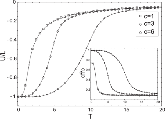
Figure 1: Internal energy for $N=100$, and connectivities $c=1,3,6$. Solid lines correspond to the exact finite size solution, Eq. (9). Symbols are the results from a Monte Carlo simulation of the canonical ensemble pertaining to the Hamiltonian of Eq. (1). Inset: maximum of magnetization, $\bar{m}$ as a function of $T$ (lines exact, symbols MC).

3 Thermodynamic limits

Assuming large $N$, with Stirling’s approximation in the form ${{a}\choose{b}}\sim\left[(b/a)^{b/a}\right.$ $\left.(1-b/a)^{1-b/a}\right]^{-a}$, and the notation $y=\frac{E}{LJ}$, Eq. (7) reads

$$Z=2^{N-2}NL(2\varphi)^{-L}\int_{-1}^{1}dm\int_{-1}^{1}dy\left[I(m,y,L,N)\right]^{L}\quad,$$ (10)

with

$$I(m,y,L,N)=\exp(-\beta Jy)\left(1-m^{2}\right)^{-\frac{1}{2c}}$$

$$\left(\frac{1-m}{1+m}\right)^{\frac{m}{2c}}\left(\frac{1-m^{4}}{1-y^{2}}\right)^{\frac{1}{2}}\left(\frac{(1-y)(1-m^{2})}{(1+y)(1+m^{2})}\right)^{\frac{y}{2}}$$

$$\times\left(1-2\varphi\frac{1-y}{1+m^{2}}\right)^{-\frac{1}{4\varphi}(1+m^{2}-2\varphi(1-y))}$$

$$\times\left(1-2\varphi\frac{1+y}{1-m^{2}}\right)^{-\frac{1}{4\varphi}(1-m^{2}-2\varphi(1+y))}\quad,$$ (11)

where $c$ and $\varphi$ are shorthands for $L/N$, and $L/N^{2}$, respectively; $h$ is set to zero for simplicity. In the thermodynamic limit $Z$ is reasonably approximated by the maximal configuration, i.e. the solution to $dI/dy=0$, which is

$$y_{\rm max}=\frac{-1-m^{2}t+\sqrt{(1+m^{2}t)^{2}-8\varphi(m^{2}-(2\varphi-1)t)t}}{4\varphi t}$$ (12)

with $t\equiv\tanh(\beta J)$. The other solution is outside the allowed parameter region of $y$. To ensure a real valued partition function the conditions, $1>2\varphi\frac{1-y}{1+m^{2}}$, and, $1>2\varphi\frac{1+y}{1-m^{2}}$, have to hold. Regions where they do not hold are forbidden zones in the $y-m$ plane, where the integrand of Eq. (10) is not defined, see Fig. 2. It can be shown that the maximum condition line, $y_{\rm max}(m)$, always stays in the allowed zone, $\forall$ $-1<m<1$, $0<t<1$, and $0<\varphi<1/2$.

For the following discussion let us compute the derivative of (the $\log$ of) $I$ in Eq. (11), with respect to $m$

$$\frac{d\log(I)}{dm}=\frac{m}{2\varphi}\log\frac{1-2\varphi\frac{1+y}{1-m^{2}}}{1-2\varphi\frac{1-y}{1+m^{2}}}+\frac{1}{2c}\log\frac{1-m}{1+m}$$ (13)

$$+ \left[\frac{1}{2}\log\frac{2\varphi(1-y^{2})-(1-y)(1-m^{2})}{2\varphi(1-y^{2})-(1+y)(1+m^{2})}-\beta J\right]y^{\prime},$$

with

$$y^{\prime}=\frac{m}{2\varphi}\left(\frac{1+m^{2}-4\varphi}{\sqrt{(1+m^{2}t)^{2}-8\varphi(m^{2}-(2\varphi-1)t)t}}-1\right)\quad.$$ (14)

It is now natural to consider two distinct thermodynamical limits, $N\to\infty$, one, by keeping connectivity $c=L/N$, the other by keeping the connectedness $\varphi=L/N^{2}$, fixed.

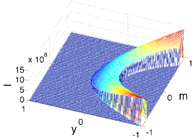
Figure 2: Logarithm of Eq. (11) in the $m-y$ plane for $\varphi=0.4$ and $c=20000$. The forbidden zones are clearly visible. The maximum is always reached in the allowed zone.

3.1 c=const. limit

We fix $c$ and take $N\to\infty$. Consequently , $\varphi$ vanishes as $1/N$, and the maximum condition from Eq. (12) reduces to

$$\lim_{\varphi\to 0}y_{\rm max}=-\frac{t+m^{2}}{1+m^{2}t}\quad.$$ (15)

The limiting cases for infinite and zero temperature can be worked out immediately.

3.1.1 The low temperature case, $\beta\gg 1$

For $J\beta\gg 1$, $t\to 1$, and the maximum condition further simplifies to, $y_{\rm max}=-1$, and $y_{\rm max}^{\prime}=\frac{2m}{1+m^{2}t}\left(\frac{t(t+m^{2})}{1+m^{2}t}-1\right)$. Using this in Eq. (13), and setting $\frac{d\log(I)}{dm}=0$ yields

$$\frac{1-m}{1+m}=\exp\left(-\frac{4cm}{1+m^{2}}\right)\quad.$$ (16)

The self-consistent solution is shown in Fig. 3(a): We find zero magnetization below a critical connectivity $c<1/2$, as well as a region where $m\neq 0$. One can show allah_private that Eq. (16) can be obtained from the results pertaining to the grand-canonical ensemble studied in allahverdyan in the limit of an infinitely large chemical potential.

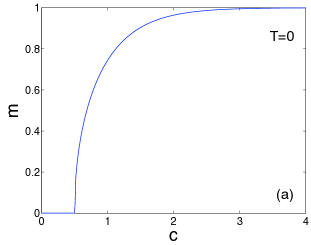
Figure 3: Fixed-$c$ thermodynamic limit. (a) Magnetization $m$ as a function of connectivity $c$ at zero temperature for $J=1$. Below $c=1/2$ there is no possibility for magnetization in the system. At $c\sim 4$, practically full magnetization is reached. (b) Phase diagram in the $T-c$ plane for $J=1$.

3.1.2 Infinite temperature, $\beta\ll 1$

For $J\beta\ll 1$, the maximum condition here becomes, $y_{\rm max}=-m^{2}$, and $y_{\rm max}^{\prime}=-2m$. Proceeding as , from $d\log(I)/dm=0$, we get $\log\left(\frac{1-m}{1+m}\right)=-4cm\beta J$, or $m=\tanh(2cm\beta J)$. This implies no magnetization for small $\beta$, or $T\to\infty$, $\forall c$. The phase transition line, separating the phases $m=0$ and $m\neq 0$, is found by noting in Eq. (11) that for $c=$const.

$$\lim_{N\to\infty}I(m,y,L,N)=e^{(1-\beta Jy)}\left(1-m^{2}\right)^{-\frac{1}{2c}}$$

$$\times\left(\frac{1-m}{1+m}\right)^{\frac{m}{2c}}\left(\frac{1-m^{4}}{1-y^{2}}\right)^{\frac{1}{2}}\left(\frac{(1-y)(1-m^{2})}{(1+y)(1+m^{2})}\right)^{\frac{y}{2}}\quad.$$ (17)

Differentiating Eq. (17) w.r.t. $m$, and setting it to zero, i.e.

$$0 = \frac{1}{2c}\log\frac{1-m}{1+m}-2m\frac{y+m^{2}}{1-m^{4}}+\frac{m(t^{2}-1)}{(1+m^{2}t)^{2}}$$ (18)

$$\times \left[\log\frac{1-y}{1+y}+\log\frac{1-m^{2}}{1+m^{2}}-2\beta J\right]\quad,$$

reduces for $m\to 0$ to the critical line given by

$$\frac{1}{2c}=\tanh\left(\frac{J}{T_{\rm c}}\right)\quad.$$ (19)

Here we used $\lim_{m\to 0}y_{\rm max}=\lim_{m\to 0}-\frac{m^{2}+t}{1+m^{2}t}=-t$. The phase diagram is shown in Fig. 3(b).

Let us finish the $c=$const. case with a statement on the critical exponent $\beta$. By inserting $y_{max}$, given in Eq. (15), into Eq. (18), we get

$$t=\frac{\log\frac{1+m}{1-m}}{4mc-m^{2}\log\frac{1+m}{1-m}}\quad.$$ (20)

Define $\tau=\frac{T_{c}-T}{T_{c}}>0$, where $T=1/\beta$. Using the Ansatz $m=\lambda\tau^{\beta}$, where $\lambda$ is a free parameter, in Eq. (20), for $\tau\ll 1$ one gets the expression

$$\frac{12c\left(1-\frac{1}{4c^{2}}\right)}{1+\frac{1}{2c}}=\lambda^{2}\tau^{2\beta-1}\quad.$$ (21)

Since the left hand side does not depend on $\tau$, the only possible choice for the critical exponent is $\beta=1/2$. This is exactly the mean field value.

3.2 $\varphi=$const. limit

Fixed $\varphi$ means diverging $c$, for $N\to\infty$.

3.2.1 The low temperature case, $\beta\gg 1$

For $J\beta\gg 1$, the second term on the right hand side of Eq. (13) vanishes. A lengthy but trivial calculation shows that Eq. (13), without that term, is larger than zero for $0<m<1$, $\forall$ $0<\varphi<1/2$, and $\forall$ $0<t<1$, where we used the fact that $y+m^{2}\leq 0$. By symmetry, Eq. (13) (without the term $\sim 1/c$) is negative for $-1<m<0$. This means there is no phase transition in the thermodynamic limit for $\varphi={\rm const.}$ and the system is always in a state of maximum magnetization, $m=\pm 1$.

3.2.2 The high temperature case, $\beta\ll 1$

For $J\beta\ll 1$, we have $t=\tanh(J\beta)\sim J\beta$, and $y_{\rm max}=-m^{2}$, and $y_{\rm max}^{\prime}=-2m$, as above. Setting $\frac{d\log(I)}{dm}=0$ in Eq. (13), we get

$$m=\tanh(2m\beta J\varphi N)\quad,$$ (22)

which means $m=1$ in the thermodynamic limit. Note, that for the case where the coupling scales as $J=J_{0}/N$, we get a phase transition, for finite $J_{0}$, which is well known for the complete graph, i.e. $\varphi=1/2$. In the context here, $\varphi$ shifts the phase transition.

More generally, assume that the coupling scales with system size as $J=J_{0}N^{a}$, with $a\leq 0$, i.e. coupling decreases with size. Assume further that $c$ scales as $c=c_{0}N^{b}$, with $b\geq 0$, then $\varphi=c_{0}N^{b-1}$. Using Eq. (22) this means

$$m=\tanh(2m\beta J_{0}c_{0}N^{a+b})\quad.$$ (23)

We see that for $a=-b$, $\kappa=2\beta J_{0}c_{0}$ can be seen as the critical parameter. For $a>-b$ we get $m=\pm 1$, whereas for $a<-b$ there is no magnetization, $m=0$.

4 Conclusion

The crucial observation of this paper is that the summation over all topologies in the Ising model on dynamical networks is equivalent to re-writing the partition function as a sum over all magnetizations. The model – which can be seen as a toy model for a variety of socio-economical situations – thus drastically reduces in complexity and becomes exactly solvable, both for finite size and the two possible thermodynamic limits.

We thank A. Allahverdyan and an anonymous referee for various most useful and clarifying comments. Supported by Austrian Science Fund FWF Projects P17621 and P19132.

References

- (1) C. Biely, K. Dragosits, S. Thurner, Physica D 228 (2007) 40.
- (2) D. Sherrington, S. Kirkpatrick, Phys. Rev. Lett. 35 (1975) 1792.
- (3) M. Idzumi, J. Phys. A: Math. Gen. 27 (1994) 27.
- (4) A.C.C. Coolen, R.W. Penney, D. Sherrington, Phys. Rev. B 48 (1993) 16116, J. Phys. A: Math. Gen. 26 (1993) 3681.
- (5) A.E. Allahverdyan, K.G. Petrosyan, Europhys. Lett. 75 (2006) 908.
- (6) A.E. Allahverdyan, T.M. Nieuwenhuizen, D.B. Saakian, Europhys. Lett. 16 (2000) 317.
- (7) J.V. Lopes, J.G. Pogorelov, J.M.B Lopes dos Santos, Phys. Rev. E 70 (2004) 026112.
- (8) T. Hasegawa, K. Nemoto, Phys. Rev. E 75 (2007) 026105.
- (9) S.N. Dorogovtsev, A.V. Goltsev A.V., J.F.F Mendes, Phys. Rev. E 66 (2002) 016104; M. Bauer, S. Coulomb, S.N. Dorogovtsev, Phys. Rev. Lett. 94 (2005) 200602; C.V. Giuraniuc et al., Phys. Rev. Lett. 95 (2005) 098701; M. Hinczewski, A.N. Berker, Phys. Rev. E 73 (2006) 066126.
- (10) J. Berg, M.Lässig, Phys. Rev. Lett. 89 (2002) 228701; Z. Burda, A. Krzywicki, Phys. Rev. E 67 (2003) 046118; J. Park, M.E.J. Newman, Phys. Rev. E 70 (2004) 066117; G. Palla, I. Derenyi, I. Farkas,T. Vicsek, Phys. Rev. E 69 (2004) 046117; C. Biely, S. Thurner, Phys. Rev. E 74 (2006) 06616.
- (11) A.E. Allahverdyan, private communication (2007).