Quasiparticle mirages in the tunneling spectra of d-wave superconductors

Abstract

We illustrate the importance of many-body effects in the Fourier transformed local density of states (FT-LDOS) of d-wave superconductors from a model of electrons coupled to an Einstein mode with energy $\Omega_{0}$. For bias energies significantly larger than $\Omega_{0}$ the quasiparticles have short lifetimes due to this coupling, and the FT-LDOS is featureless if the electron-impurity scattering is treated within the Born approximation. In this regime it is important to include boson exchange for the electron-impurity scattering which provides a ‘step down’ in energy for the electrons and allows for long lifetimes. This many-body effect produces qualitatively different results, namely the presence of peaks in the FT-LDOS which are mirrors of the quasiparticle interference peaks which occur at bias energies smaller than $\sim\Omega_{0}$. The experimental observation of these quasiparticle mirages would be an important step forward in elucidating the role of many-body effects in FT-LDOS measurements.

Many-body effects are known to influence the electron spectral function in cuprates, in particular the peak-dip-hump lineshape seen in the superconducting state by both angle resolved photoemission and tunneling eschrigreview . The nature of the bosonic modes that give rise to this lineshape is a topic of much debate. Among the possibilities that have been discussed in the literature are certain optical phonons, as well as the spin resonance seen by inelastic neutron scattering. They all have a comparable excitation energy, $\Omega_{0}\approx 40$ meV for optimal doped Bi₂Sr₂CaCu₂O_8+δ (Bi2212), which is also near the energy of the antinodal gap, $\Delta_{A}$. Very recently it has been suggested that scanning tunneling spectroscopy (STS) can be useful in revealing the electron-boson coupling in the cuprates jlee . In STS the differential conductance $dI/dV({\bf r},eV)$ is a measure of the local density of states (LDOS) $\rho({\bf r},\omega=eV)$ of the electrons, while the Fourier transform (${\bf r}\rightarrow{\bf q}$) yields $\rho({\bf q},\omega)$ (FT-LDOS). The location of the peaks of $\rho({\bf q},\omega)$ provides information about the excitation spectrum of the electronic states hoffman ; kyle . In view of the suggestion of Ref. jlee, , it is particularly important to carefully examine how electron-boson coupling affects these peaks balatsky .

Modulations of the LDOS and the concomitant peaks in $\rho({\bf q},\omega)$ are due to electrons scattering from impurities. In most studies the electron-impurity scattering has been treated either within a $T$-matrix approximation wanglee or a Born approximation capriotti . In this framework, the peaks in $\rho({\bf q},\omega)$ appear at wavevectors ${\bf q}={\bf k}_{f}-{\bf k}_{i}$, where ${\bf k}_{f}$ and ${\bf k}_{i}$ are points of high density of states at the energy $\omega$. This approach has been quite successful in understanding FT-LDOS data for $|\omega|\lesssim\Delta_{A}$, and has been denoted as the ‘octet’ model kyle . We note that the success of this approach depends on the existence of electronic states with long lifetimes in this energy range. Subsequent to this, there have been attempts to go beyond these approximations by including the interaction of the electrons with either phonons or spin fluctuations balatsky ; polkovnikov .

The purpose of this paper is to reveal that for bias energies greater than $\sim\Delta_{A}$, where no quasiparticles are observed in photoemission arpes , there can be sharp peaks in $\rho({\bf q},\omega)$ due to a boson exchange process that appears beyond the Born approximation for the electron-impurity scattering. For $|\omega|>\Omega_{0}$, an electron can decay into a lower energy state by emitting a boson of energy $\Omega_{0}$. As a result, the lifetime of the electrons with energy $\omega$ significantly larger than $\Omega_{0}$ is severely reduced, which is the primary reason for the absence of sharp peaks in $\rho({\bf q},\omega)$ at the level of the Born approximation. But, going beyond the Born approximation in the process shown in Fig. 1b, an electron first emits a boson which reduces its energy to $|\omega|-\Omega_{0}$. If this reduced energy is not significantly larger than $\Omega_{0}$, the resulting electron state (the internal fermion line of the diagram) is once again long-lived, and consequently contributes to peaks in $\rho({\bf q},\omega)$ by scattering from the impurities. In this process, the location of the peaks at $\omega$ is determined by the excitation spectrum at an energy $(|\omega|-\Omega_{0})\rm{sgn}(\omega)$. That is, one has mirages of the octet peaks at $|\omega_{QI}|\lesssim\Delta_{A}$ that are mirrored at an energy $|\omega_{QM}|=|\omega_{QI}|+\Omega_{0}$. We note that this argument is based entirely on the energetics of the electron-boson interaction, and does not depend on the momentum space structure of the bosons (i.e., whether the bosons are spin fluctuations peaked at large wavevectors or phonons peaked at small wavevectors), though of course the momentum form factor of the bosons will lead to quantitative differences.

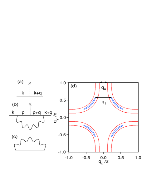
Figure 1: (Color online) Panels (a)-(c) show the relevant diagrams considered in this paper: Born diagram, vertex correction, and the self-energy, respectively. The cross represents an impurity and the wiggly line a boson. In (a) and (b) the electrons (straight lines) are dressed by the self-energy. In (c) the electron line is bare. Panel (d) shows the constant energy contours of the bare dispersion for two energies: $-\omega=20$ meV (the closed ‘banana’ contour) and $-\omega=76$ meV (the open contours), noting that $\Delta_{A}=37$ meV. The wavevector ${\bf q}_{1}$ connects the tips of the closed contour, and ${\bf q}_{A}$ connects the inner of the two open contours along the antinodal direction.

Model. We study a two-dimensional system of superconducting electrons described by a BCS model interacting with a boson mode, and coupled to an isotropic potential scatterer. It is described by the Hamiltonian $\mathcal{H}=\mathcal{H}_{BCS}+\mathcal{H}_{im}+\mathcal{H}_{el-b}$. Here $\mathcal{H}_{BCS}=\sum_{{\bf k},\sigma}\epsilon_{{\bf k}}c^{\dagger}_{{\bf k}\sigma}c_{{\bf k}\sigma}+\sum_{{\bf k}}\Delta_{{\bf k}}(c^{\dagger}_{{\bf k}\uparrow}c^{\dagger}_{-{\bf k}\downarrow}+c_{-{\bf k}\downarrow}c_{{\bf k}\uparrow})$, where $c^{\dagger}_{{\bf k}\sigma}$ ($c_{{\bf k}\sigma}$) creates (annihilates) electrons with spin $\sigma$ at wavevector ${\bf k}$, the normal state dispersion is given by the tight binding expansion $\epsilon_{{\bf k}}=t_{0}+t_{1}(\cos k_{x}+\cos k_{y})/2+t_{2}\cos k_{x}\cos k_{y}+t_{3}(\cos 2k_{x}+\cos 2k_{y})/2+t_{4}(\cos 2k_{x}\cos k_{y}+\cos k_{x}\cos 2k_{y})/2+t_{5}\cos 2k_{x}\cos 2k_{y}$, and the superconducting gap has the d-wave form $\Delta_{{\bf k}}=\Delta_{M}(\cos k_{x}-\cos k_{y})/2$, with the lattice constant set to unity ($M$ denoting the $(\pi,0)$ point). In order to study the sensitivity of $\rho({\bf q},\omega)$ to the dispersion, we considered two sets of values for the parameters $t_{i}$, one taken from Ref. eschrig, and the other from Ref. kaminski, . For both dispersions, the antinode is at ${\bf k}_{A}=(1,0.18)\pi$. They differ in that the first dispersion has $\epsilon_{M}$ close to the Fermi energy (-34 meV), whereas it is further away for the second (-119 meV). We focus here on results from the second dispersion, though qualitatively similar results were obtained from the first. For $\Delta_{M}$, we choose 40 meV, a typical value for optimal doped Bi2212.

The electron-impurity scattering is given by $\mathcal{H}_{im}=V_{0}\sum_{{\bf k},{\bf q},\sigma}c^{\dagger}_{{\bf k}+{\bf q}\sigma}c_{{\bf k}\sigma}$, where $V_{0}=1$eV in our calculation (note that $V_{0}$ simply sets the scale for the FT-LDOS). For the sake of concreteness, we take the coupling between the bosons and the electrons to be of the form $\mathcal{H}_{el-b}=g\sum_{i}{\bf S}_{i}\cdot{\bf s}_{i}$, where ${\bf S}_{i}$ and ${\bf s}_{i}$ are the spin fluctuation and the electron spin operators respectively at site $i$, though our results hold equally well for optical phonons. We fix the magnitude of the coupling constant $g$ from the condition that in the normal state ($\Delta_{{\bf k}}=0$) the inverse quasi-particle weight $z^{-1}=1-\frac{\partial{\rm Re}\Sigma(\omega)}{\partial\omega}\approx 2$ at the Fermi energy, where $\Sigma(\omega)$ is the electron self-energy due to interaction with the spin fluctuations. This gives $3g^{2}=0.0176$ eV². The dynamics of the spin fluctuations is given by $\chi_{\mu\nu}({\bf Q},i\Omega_{n})=\chi(i\Omega_{n})\delta_{\mu\nu}$, with $\chi(i\Omega_{n})=2\Omega_{0}/(\Omega_{n}^{2}+\Omega_{0}^{2})$, where $\chi_{\mu\nu}({\bf Q},\tau)=\langle T_{\tau}S_{\mu}({\bf Q},\tau)S_{\nu}(-{\bf Q},0)\rangle$ is the spin fluctuation propagator (the overall prefactor being absorbed into the definition of $g$). Here $\mu$, $\nu$ are spatial indices, $\Omega_{n}$ is a bosonic Matsubara frequency, and the mode energy $\Omega_{0}$ is taken to be 39 meV. In our model, we take the bosons to be independent of momentum for the following reasons. First, it allows us to concentrate on the energetics. As discussed in Ref. eschrig, , as long as the form factor of the bosons is finite throughout the zone, then the self-energy will be dominated by the density of states singularities associated with the antinodal and $M$ points of the internal fermion line. Second, it greatly simplifies the calculation of the vertex diagram (Fig. 1b).

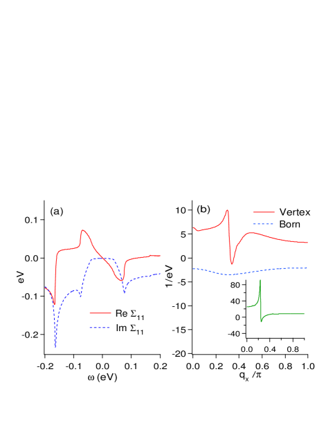
Figure 2: (Color online) (a) The real and imaginary parts of the 11 component of the self-energy. (b) Contribution to the FT-LDOS from the vertex diagram for $-\omega=\Omega_{0}+\Delta_{A}=76$ meV. The dashed line shows the contribution from the Born diagram. The inset shows the contribution from the Born diagram for electrons without the self-energy correction.

Using Nambu notation, the $2\times 2$ electron Green’s function with self-energy correction (Fig. 1c) is given by

$$G^{-1}({\bf k},z)=\left[\begin{array}[]{cc}z-\epsilon_{{\bf k}}-\Sigma_{11}(z)&-\Delta_{{\bf k}}-\Sigma_{12}({\bf k},z)\\ -\Delta_{{\bf k}}-\Sigma_{12}^{*}({\bf k},z)&z+\epsilon_{{\bf k}}-\Sigma_{22}(z)\end{array}\right],$$

where $z$ is the complex frequency. The diagonal self-energies at T=0 are given by eschrig $\Sigma_{11/22}(z)=3g^{2}\sum_{{\bf k}}[z\pm\epsilon_{{\bf k}}(1+\Omega_{0}/E_{{\bf k}})]/[z^{2}-(\Omega_{0}+E_{{\bf k}})^{2}]$, where $E_{{\bf k}}=\sqrt{\epsilon_{{\bf k}}^{2}+\Delta_{{\bf k}}^{2}}$. In the above, the ${\bf k}$-summation is performed numerically with an intrinsic lifetime broadening factor $\eta=2$ meV for $z=\omega+i\eta$. In Fig. 2a we show the real and imaginary components of $\Sigma_{11}(z)$ as a function of $\omega$. ${\rm Im}\Sigma_{11}(\omega)$ is zero for $|\omega|\lesssim\Omega_{0}$, and has pronounced peaks at $|\omega|=\Omega_{0}+\Delta_{A}$ and $\Omega_{0}+E_{M}$. Consequently, for energies up to and slightly beyond $\Omega_{0}$, the electronic states form well defined quasiparticles, while for $|\omega|\gg\Omega_{0}$ they do not. Strictly speaking, for momentum independent bosons, the off-diagonal self-energies vanish due to the $d$-wave symmetry. However, in order to keep the antinode gap energy unrenormalized, we use the ansatz $\Sigma_{12}({\bf k},\omega)=\Delta_{{\bf k}}[Z({\omega})-1]$, where $Z(\omega)=1-\frac{1}{2\omega}{\rm Re}[\Sigma_{11}(\omega)+\Sigma_{22}(\omega)]$. In this scheme, the renormalized dispersion is $\tilde{E}_{{\bf k}}\approx[\Delta_{{\bf k}}^{2}+\epsilon_{{\bf k}}^{2}/Z^{2}(\tilde{E}_{{\bf k}})]^{1/2}$.

Results. We first compute the contribution to the FT-LDOS from the Born diagram (Fig. 1a). This is given by $\rho^{(b)}({\bf q},\omega)=-(2/\pi){\rm Im}[V_{0}\sum_{{\bf k}}G_{1\alpha}^{R}({\bf k},\omega)(\hat{\tau}_{3})_{\alpha\beta}G_{\beta 1}^{R}({\bf k}+{\bf q},\omega)]$, where summation over repeated Nambu indices $\alpha,\beta=(1,2)$ is implied, and $\hat{\tau}_{i}$ are Pauli matrices in Nambu space, with $R$ denoting retarded propagators. The variation of $\rho^{(b)}({\bf q},\omega)$ versus ${\bf q}=(q_{x},0)$ is shown as the dashed curve in Fig. 2b for $-\omega=\Delta_{A}+\Omega_{0}$. We note that, due to large lifetime broadening, there is no peak in $\rho^{(b)}({\bf q},\omega)$ at this energy. The effect of the lifetime can be seen clearly by comparing this curve with the one in the inset which is obtained by computing $\rho^{(b)}({\bf q},\omega=-\Omega_{0}-\Delta_{A})$ with $\hat{\Sigma}=0$ (i.e., for unrenormalized electrons).

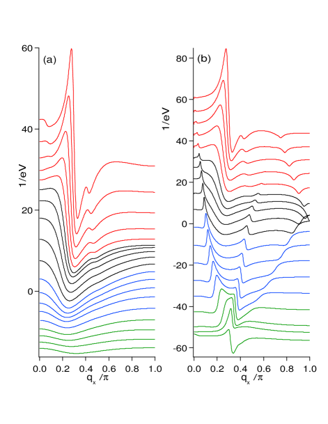
Figure 3: (Color online) (a) Born contribution, and (b) Born plus vertex contributions, to the FT-LDOS for energies ranging from near $-\Omega_{0}$ (-40 meV, top curve) to $-\Omega_{0}-\Delta_{A}$ (-76 meV, bottom curve) in steps of 2 meV. The curves are offset for clarity.

Next we calculate the FT-LDOS contribution of the vertex diagram (Fig. 1b). This is given by

$$\rho^{(v)}({\bf q},\omega) = -\left(\frac{2}{\pi}\right){\rm Im}\left[V_{0}\sum_{{\bf k}}G_{1\alpha}^{R}({\bf k},\omega)T_{\alpha\beta}^{R}({\bf q},\omega)\right.$$ (1)

$$\times \left.G_{\beta 1}^{R}({\bf k}+{\bf q},\omega)\right],$$

where

$$T_{\alpha\beta}({\bf q},i\omega_{n}) = \frac{3g^{2}}{\beta}\sum_{\Omega_{n},{\bf p}}\chi(i\Omega_{n})G_{\alpha\gamma}({\bf p},i\omega_{n}-i\Omega_{n})$$

$$\times (\hat{\tau}_{3})_{\gamma\delta}G_{\delta\beta}({\bf p}+{\bf q},i\omega_{n}-i\Omega_{n}).$$

Here $\beta$ is the inverse temperature and $\omega_{n}$ is a fermionic Matsubara frequency. We note that in our model, the matrix $\hat{T}$ does not depend on ${\bf k}$ due to the momentum independence of the bosons. The variation of $\rho^{(v)}({\bf q},\omega)$ along the bond direction is plotted in Fig. 2b for $\omega=-(\Omega_{0}+\Delta_{A})$. We note the pronounced structure with a sharp maximum at $q_{x}=0.30\pi$ and a sharp minimum at $0.34\pi$. As $|\omega|$ increases from $\omega=-(\Omega_{0}+\Delta_{A})$ to $-(\Omega_{0}+\tilde{E}_{M})$, where $\tilde{E}_{M}$ is the renormalized energy at the $M$ point ($\sim$ 60 meV), this structure evolves into a single broad minimum at $q_{x}=0.23\pi$ (not shown). This can be contrasted with the Born result, where there is only weak structure in this entire energy range.

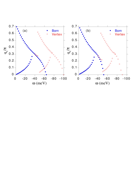
Figure 4: (Color online) Dispersion of the the Fourier peaks along the bond direction versus energy for (a) the real part and (b) the imaginary part of the Born and vertex diagrams. Note the characteristic ‘$\lambda$’ shape of the Born dispersion and its $\Omega_{0}$ (39 meV) displaced ‘mirage’ in the vertex dispersion.

For $|\omega|\gg\Omega_{0}$, due to a large ${\rm Im}\Sigma_{\alpha\alpha}(\omega)$, the ${\bf k}$-summation in Eq. (1) involving the product of two $G$ functions yields a quantity (denoted as $C$) which is approximately constant as a function of ${\bf q}$. The variation of $\rho^{(v)}({\bf q},\omega)$ with ${\bf q}$ for these energies is mainly due to that of $T_{\alpha\beta}^{R}({\bf q},\omega)$. For the frequency summation involved in the computation of $T_{\alpha\beta}^{R}({\bf q},\omega)$, the main contribution is due to the bosonic pole which puts the electrons with momentum ${\bf p}$ and ${\bf p}+{\bf q}$ (Fig. 1b) at an energy $\omega+\Omega_{0}$ for $\omega$ negative. This contribution can be written as (for $\omega<-\Omega_{0}$) $\hat{T}^{R}({\bf q},\omega)_{{\rm coh}}=3g^{2}\sum_{{\bf p}}\hat{G}({\bf p},\omega+\Omega_{0})\hat{\tau}_{3}\hat{G}({\bf p}+{\bf q},\omega+\Omega_{0}).$ This expression is reminiscent of the Born contribution at an energy $\omega+\Omega_{0}$, and gives rise to sharp structure for $|\omega|-\Omega_{0}\lesssim\Omega_{0}$ since the electronic states are well defined at these energies.

To understand this in greater detail, we plot in Fig. 3a the contribution to the FT-LDOS from the Born diagram, and in Fig. 3b the sum of the Born and vertex contributions, versus $(q_{x},0)$, for $\Omega_{0}<|\omega|<\Omega_{0}+\Delta_{A}$. In Fig. 4, we in turn plot the resulting peak dispersions from the real and imaginary parts of the Born and vertex diagrams for all $|\omega|<\Omega_{0}+\tilde{E}_{M}$. We note that the Born dispersion is well defined in the energy range between 0 and $\tilde{E}_{M}$, although the Born peaks are damped for $\Omega_{0}<|\omega|<\tilde{E}_{M}$ due to lifetime broadening. For $|\omega|<\Delta_{A}$, there are two peaks. The one at larger $q_{x}$ corresponds to scattering between the tips of the of the constant energy contours, which look like bananas in this energy range. This is denoted by the vector ${\bf q}_{1}$ in Fig. 1d (structure corresponding to the even larger vector ${\bf q}_{5}$ of Ref. kyle, is not plotted in Fig. 4). The one at smaller $q_{x}$ corresponds to the so-called Tomasch peak noted in Ref. capriotti, . It corresponds to where the banana first stops overlapping its $q_{x}$ displaced image. For $\Delta_{A}<|\omega|<\tilde{E}_{M}$, one finds a dominant maximum which traces out the separation of the inner contours in Fig. 1d along the antinodal ($(\pi,0)-(\pi,\pi)$) direction (denoted as ${\bf q}_{A}$ in Fig. 1d), with secondary peaks (not plotted in Fig. 4) corresponding to connecting an inner to an outer contour or an outer to an outer contour (these secondary peaks have less weight due to the reduced spectral weight of the outer contours). The combination of these peaks (two for $|\omega|<\Delta_{A}$ and one for $|\omega|>\Delta_{A}$) gives a characteristic ‘$\lambda$’ shape to the overall bond oriented dispersion, as is obvious from Fig. 4. Note there are some differences in the dispersions associated with the real and imaginary parts of the Born diagram and their connection to the vectors denoted in Fig. 1d. This is due to several factors: the finite lifetime of the electronic states, the dispersion $\epsilon_{k}$, and the fact that Re$G$ has a zero where Im$G$ has a pole.

We now turn to the vertex diagram. Its dispersion (Fig. 4) essentially mirrors the Born dispersion at a bias energy displaced by $\Omega_{0}$. As a consequence, we denote this as a ‘quasiparticle mirage’. In addition, for biases near $\Omega_{0}$, the energy undisplaced Born term is also reflected in the vertex diagram (since the external lines in Fig. 1b have well defined spectral peaks, and the boson exchange process has a limited phase space, for these energies). We note that there are some differences in the lineshapes of the imaginary part of the vertex term as compared to that of the Born term displaced by $\Omega_{0}$, as is evident in Fig. 3. This occurs since both the real and imaginary parts of the components of $\hat{T}$ contribute to $\rho^{(v)}({\bf q},\omega)$ as $C$ is a complex quantity.

Next, we comment on a few qualitative aspects of the vertex contribution to the FT-LDOS. (i) The inclusion of a momentum form factor for the boson propagator should not make any qualitative change to the peak structure. Such a form factor (peaked around some ${\bf Q}_{0}$) can be thought of as a momentum constraint forcing ${\bf k}\approx{\bf p}+\hat{\alpha}{\bf Q}_{0}$ (where $\hat{\alpha}$ is a lattice group operation). However, in the mechanism discussed above, the electrons with momentum ${\bf k}$ and ${\bf k}+{\bf q}$ (external lines of Fig. 1b) do not play any special role. (ii) It is important that the boson that provides the ‘step down’ in energy has a sharp spectral function. A finite lifetime of the boson, or its dispersion with $q$, will broaden the Fourier peaks. For similar reasons, we anticipate that higher order vertex corrections will lead to weaker and broader contributions to the Fourier peaks because of the additional momentum sums involved. (iii) Recently, the observation of peaks in the Fourier transformed $d^{2}I/dV^{2}$ spectrum at ${\bf q}\approx(0.4\pi,0)$ has been reported for optimal doped Bi2212 at $|\omega|\approx\Omega_{0}+\Delta_{A}$ jlee . This is comparable to the peak position we find from our vertex corrected calculation at this bias energy. So far, though, no dispersion of these peaks has been reported.

Conclusion. We demonstrated the importance of vertex corrections to electron impurity scattering in the study of tunneling spectroscopy data for the cuprate superconductors for absolute bias energies larger than $\Omega_{0}$, where $\Omega_{0}$ is the excitation energy of a boson coupled to the electrons. The vertex correction is due to emission and re-absorption of a boson by the electrons which leads to a ‘step down’ of the internal fermion line to energies where quasiparticle states are well defined, which as a consequence gives rise to sharp peaks in the FT-LDOS. We denote these new peaks as ‘quasiparticle mirages’, whose dispersion mirrors the previously observed quasiparticle interference peaks at absolute biases smaller than $\Omega_{0}$. The observation of these dispersive ‘mirages’ would be an important reflection of the nature of the many-body interactions in cuprates.

This work was supported by the U. S. Dept. of Energy, Office of Science, under Contract No. DE-AC02-06CH11357. Part of the calculations were performed at the Ohio Supercomputer Center thanks to a grant of computing time. The authors would like to thank Mohit Randeria for suggesting this work.

References

- (1) M. Eschrig, Adv. Phys. 55, 47 (2006).
- (2) J. Lee, K. Fujita, K. McElroy, J. A. Slezak, M. Wang, Y. Aiura, H. Bando, M. Ishikado, T. Masui, J.-X. Zhu, A. V. Balatsky, H. Eisaki, S. Uchida and J. C. Davis, Nature 442, 546 (2006).
- (3) J. E. Hoffman, K. McElroy, D.-H. Lee, K. M Lang, H. Eisaki, S. Uchida and J. C. Davis, Science 297, 1148 (2002).
- (4) K. McElroy, R. W. Simmonds, J. E. Hoffman, D.-H. Lee, J. Orenstein, H. Eisaki, S. Uchida and J. C. Davis, Nature 422, 592 (2003).
- (5) J.-X. Zhu, J. Sun, Q. Si and A. V. Balatsky, Phys. Rev. Lett. 92, 017002 (2004); J.-X. Zhu, K. McElroy, J. Lee, T. P. Devereaux, Q. Si, J. C. Davis and A. V. Balatsky, ibid 97, 177001 (2006); J.-X. Zhu, A. V. Balatsky, T. P. Devereaux, Q. Si, J. Lee, K. McElroy and J. C. Davis, Phys. Rev. B 73, 014511 (2006).
- (6) Q.-H. Wang and D.-H. Lee, Phys. Rev. B 67, 020511 (2003).
- (7) L. Capriotti, D. J. Scalapino and R. D. Sedgewick, Phys. Rev. B 68, 014508 (2003).
- (8) A. Polkovnikov, M. Vojta and S. Sachdev, Phys. Rev. B 65, 220509 (2002); D. Podolsky, E. Demler, K. Damle and B. I. Halperin, ibid 67, 094514 (2003); J. H. Han, ibid 67, 094506 (2003).
- (9) A. Kaminski, M. Randeria, J. C. Campuzano, M. R. Norman, H. Fretwell, J. Mesot, T. Sato, T. Takahashi and K. Kadowaki, Phys. Rev. Lett. 86, 1070 (2001).
- (10) M. Eschrig and M. R. Norman, Phys. Rev. B 67, 144503 (2003).
- (11) This dispersion is denoted as tb2 in M. R. Norman, Phys. Rev. B 75, 184514 (2007).