Encyclopedia of Mathematical Physics  (J.-P. Françoise, G. Naber, and S. T. Tsou, eds.)
Vol. 4, pp. 353–371. Elsevier, Oxford, 2006.

Random Walks in Random Environments

L. V. Bogachev, University of Leeds, Leeds, UK

© 2006 Elsevier Ltd. All rights reserved.

1 Introduction

Random walks provide a simple conventional model to describe various transport processes, for example propagation of heat or diffusion of matter through a medium (for a general reference see, e.g., Hughes (1995)). However, in many practical cases the medium where the system evolves is highly irregular, due to factors such as defects, impurities, fluctuations etc. It is natural to model such irregularities as random environment, treating the observable sample as a statistical realization of an ensemble, obtained by choosing the local characteristics of the motion (e.g., transport coefficients and driving fields) at random, according to a certain probability distribution.

In the random walks context, such models are referred to as Random Walks in Random Environments (RWRE). This is a relatively new chapter in applied probability and physics of disordered systems initiated in the 1970s. Early interest in RWRE models was motivated by some problems in biology, crystallography and metal physics, but later applications have spread through numerous areas (see review papers by Alexander et al. (1981), Bouchaud and Georges (1990), and a comprehensive monograph by Hughes (1996)). After 30 years of extensive work, RWRE remain a very active area of research, which has been a rich source of hard and challenging questions and has already led to many surprising discoveries, such as subdiffusive behavior, trapping effects, localization, etc. It is fair to say that the RWRE paradigm has become firmly established in physics of random media, and its models, ideas, methods, results, and general effects have become an indispensable part of the standard tool kit of a mathematical physicist.

One of the central problems in random media theory is to establish conditions ensuring homogenization, whereby a given stochastic system evolving in a random medium can be adequately described, on some spatial-temporal scale, using a suitable effective system in a homogeneous (non-random) medium. In particular, such systems would exhibit classical diffusive behavior with effective drift and diffusion coefficient. Such an approximation, called effective medium approximation (EMA), may be expected to be successful for systems exposed to a relatively small disorder of the environment. However, in certain circumstances EMA may fail due to atypical environment configurations (“large deviations”) leading to various anomalous effects. For instance, with small but positive probability a realization of the environment may create “traps” that would hold the particle for anomalously long time, resulting in the subdiffusive behavior, with the mean square displacement growing slower than linearly in time.

RWRE models have been studied by various non-rigorous methods including Monte Carlo simulations, series expansions, and the renormalization group techniques (see more details in the above references), but only few models have been analyzed rigorously, especially in dimensions greater than one. The situation is much more satisfactory in the one-dimensional case, where the mathematical theory has matured and the RWRE dynamics has been understood fairly well.

The goal of this article is to give a brief introduction to the beautiful area of RWRE. The principal model to be discussed is a random walk with nearest-neighbor jumps in independent identically distributed (i.i.d.) random environment in one dimension, although we shall also comment on some generalizations. The focus is on rigorous results; however, heuristics will be used freely to motivate the ideas and explain the approaches and proofs. In a few cases, sketches of the proofs have been included, which should help appreciate the flavor of the results and methods.

1.1 Ordinary Random Walks: A Reminder

To put our exposition in perspective, let us give a brief account of a few basic concepts and facts for ordinary random walks, that is, evolving in a non-random environment (see further details in Hughes 1995). In such models, space is modelled using a suitable graph, e.g., a $d$-dimensional integer lattice $\mathbb{Z}^{d}$, while time may be discrete or continuous. The latter distinction is not essential, and in this article we will mostly focus on the discrete-time case. The random mechanism of spatial motion is then determined by the given transition probabilities (probabilities of jumps) at each site of the graph. In the lattice case, it is usually assumed that the walk is translation invariant, so that at each step distribution of jumps is the same, with no regard to the current location of the walk.

In one dimension ($d=1$), the simple (nearest-neighbor) random walk may move one step to the right or to the left at a time, with some probabilities $p$ and $q=1-p$, respectively. An important assumption is that only the current location of the walk determines the random motion mechanism, whereas the past history is not relevant. In terms of probability theory, such a process is referred to as Markov chain. Thus, assuming that the walk starts at the origin, its position after $n$ steps can be represented as the sum of consecutive displacements, $X_{n}=Z_{1}+\dots+Z_{n}$, where $Z_{i}$ are independent random variables with the same distribution $P\{Z_{i}=1\}=p$,  ${P\{Z_{i}=-1\}=q}$.

The strong law of large numbers (LLN) states that almost surely (i.e., with probability $1$)

$$\lim_{n\to\infty}\frac{X_{n}}{n}=\operatorname{\mathit{E}}Z_{1}=p-q,\quad\operatorname{\mathit{P}}\text{-a.s.}$$ (1)

where $\operatorname{\mathit{E}}$ denotes expectation (mean value) with respect to $\operatorname{\mathit{P}}$. This result shows that the random walk moves with the asymptotic average velocity close to $p-q$. It follows that if $p-q\neq 0$ then the process $X_{n}$, with probability 1, will ultimately drift to infinity (more precisely, $+\infty$ if $p-q>0$ and $-\infty$ if $p-q<0$). In particular, in this case the random walk may return to the origin (and in fact visit any site on $\mathbb{Z}$) only finitely many times. Such behavior is called transient. However, in the symmetric case (i.e., $p=q=0.5$) the average velocity vanishes, so the above argument fails. In this case the walk behavior appears to be more complicated, as it makes increasingly large excursions both to the right and to the left, so that $\varlimsup_{n\to\infty}X_{n}=+\infty$,  $\varliminf_{n\to\infty}X_{n}=-\infty$ ($\operatorname{\mathit{P}}$-a.s.). This implies that a symmetric random walk in one dimension is recurrent, in that it visits the origin (and indeed any site on $\mathbb{Z}$) infinitely often. Moreover, it can be shown to be null-recurrent, which means that the expected time to return to the origin is infinite. That is to say, return to the origin is guaranteed, but it takes very long until this happens.

Fluctuations of the random walk can be characterized further via the central limit theorem (CLT), which amounts to saying that the distribution of $X_{n}$ is asymptotically normal, with mean $n(p-q)$ and variance $4npq$:

$$\lim_{n\to\infty} \operatorname{\mathit{P}}\left\{\frac{X_{n}-n(p-q)}{\sqrt{4npq}}\leq x\right\}$$

$$=\varPhi(x):=\frac{1}{\sqrt{2\pi}}\int_{-\infty}^{x}{\mathrm{e}}^{-y^{2}/2}\,{\mathrm{d}}y.$$ (2)

These results can be extended to more general walks in one dimension, and also to higher dimensions. For instance, the criterion of recurrence for a general one-dimensional random walk is that it is unbiased, $\operatorname{\mathit{E}}(X_{1}-X_{0})=0$. In the two-dimensional case, in addition one needs $\operatorname{\mathit{E}}|X_{1}-X_{0}|^{2}<\infty$. In higher dimensions, any random walk (which does not reduce to lower dimension) is transient.

1.2 Random Environments and Random
Walks

The definition of an RWRE involves two ingredients: (i) the environment, which is randomly chosen but remains fixed throughout the time evolution, and (ii) the random walk, whose transition probabilities are determined by the environment. The set of environments (sample space) is denoted by $\Omega=\{\omega\}$, and we use $\operatorname{\mathbb{P}}$ to denote the probability distribution on this space. For each $\omega\in\Omega$, we define the random walk in the environment $\omega$ as the (time-homogeneous) Markov chain $\{X_{t},\,t=0,1,2,\dots\}$ on $\mathbb{Z}^{d}$ with certain (random) transition probabilities

$$p(x,y,\omega)=\operatorname{\mathit{P}}^{\omega}\{X_{1}=y\,|\,X_{0}=x\}.$$ (3)

The probability measure $\operatorname{\mathit{P}}^{\omega}$ that determines the distribution of the random walk in a given environment $\omega$ is referred to as the quenched law. We often use a subindex to indicate the initial position of the walk, so that e.g. $\operatorname{\mathit{P}}^{\omega}_{x}\{X_{0}=x\}=1$.

By averaging the quenched probability $\operatorname{\mathit{P}}^{\omega}_{x}$ further, with respect to the environment distribution, we obtain the annealed measure $\operatorname{\mbox{\boldmath$P$}}_{x}=\operatorname{\mathbb{P}}\times\operatorname{\mathit{P}}^{\omega}_{x}$, which determines the probability law of the RWRE:

$$\operatorname{\mbox{\boldmath$P$}}_{x}(A)=\int_{\Omega}\operatorname{\mathit{P}}_{x}^{\omega}(A)\operatorname{\mathbb{P}}({\mathrm{d}}\omega)=\operatorname{\mathbb{E}}\operatorname{\mathit{P}}_{x}^{\omega}(A).$$ (4)

Expectation with respect to the annealed measure $\operatorname{\mbox{\boldmath$P$}}_{x}$ will be denoted by $\operatorname{\mbox{\boldmath$E$}}_{x}$.

Equation (4) implies that if some property $A$ of the RWRE holds almost surely (a.s.) with respect to the quenched law $\operatorname{\mathit{P}}_{x}^{\omega}$ for almost all environments (i.e., for all $\omega\in\Omega^{\prime}$ such that $\operatorname{\mathbb{P}}(\Omega^{\prime})=1$), then this property is also true with probability $1$ under the annealed law $\operatorname{\mbox{\boldmath$P$}}_{x}$.

Note that the random walk $X_{n}$ is a Markov chain only conditionally on the fixed environment (i.e., with respect to $\operatorname{\mathit{P}}_{x}^{\omega}$), but the Markov property fails under the annealed measure $\operatorname{\mbox{\boldmath$P$}}_{x}$. This is because the past history cannot be neglected, as it tells what information about the medium must be taken into account when averaging with respect to environment. That is to say, the walk learns more about the environment by taking more steps. (This idea motivates the method of “environment viewed from the particle”, see Section 7 below.)

The simplest model is the nearest-neighbor one-dimensional walk, with transition probabilities

$$p(x,y,\omega)=\left\{\begin{array}[]{ll}p_{x}&\text{if}\ \ y=x+1,\\ q_{x}&\text{if}\ \ y=x-1,\\ 0&\text{otherwise},\end{array}\right.$$

where $p_{x}$ and $q_{x}=1-p_{x}$ ($x\in\mathbb{Z}$) are random variables on the probability space $(\Omega,\operatorname{\mathbb{P}})$. That is to say, given the environment $\omega\in\Omega$, the random walk currently at point $x\in\mathbb{Z}$ will make a one-unit step to the right, with probability $p_{x}$, or to the left, with probability $q_{x}$. Here the environment is determined by the sequence of random variables $\{p_{x}\}$. For the most of the article, we assume that the random probabilities $\{p_{x},\,x\in\mathbb{Z}\}$ are independent and identically distributed (i.i.d.), which is referred to as i.i.d. environment. Some extensions to more general environments will be mentioned briefly in Section 9. The study of RWRE is simplified under the following natural condition called (uniform) ellipticity:

$$0<\delta\leq p_{x}\leq 1-\delta<1,\ \ x\in\mathbb{Z},\quad\operatorname{\mathbb{P}}\text{-a.s.}$$ (5)

which will be frequently assumed in the sequel.

2 Transience and Recurrence

In this section, we discuss a criterion for the RWRE to be transient or recurrent. The following theorem is due to Solomon (1975).

Theorem 1.

Set $\rho_{x}:=q_{x}/p_{x}$, $x\in\mathbb{Z}$, and $\eta:=\operatorname{\mathbb{E}}\ln\rho_{0}$.

(i) If $\eta\neq 0$ then $X_{t}$ is transient ($\operatorname{\mbox{\boldmath$P$}}_{0}$-a.s.); moreover, if $\eta<0$ then $\lim_{t\to\infty}X_{t}=+\infty$, while if $\eta>0$ then $\lim_{t\to\infty}X_{t}=-\infty$ ($\operatorname{\mbox{\boldmath$P$}}_{0}$-a.s.).

(ii) If $\eta=0$ then $X_{t}$ is recurrent ($\operatorname{\mbox{\boldmath$P$}}_{0}$-a.s.); moreover,

$$\varlimsup_{t\to\infty}X_{t}=+\infty,\quad\varliminf_{t\to\infty}X_{t}=-\infty,\quad\operatorname{\mbox{\boldmath$P$}}_{0}\text{-a.s.}$$

Let us sketch the proof. Consider the hitting times $T_{x}:=\min\{t\geq 0:X_{t}=x\}$ and denote by $f_{xy}$ the quenched first-passage probability from $x$ to $y$:

$$f_{xy}:=\operatorname{\mathit{P}}^{\omega}_{x}\{1\leq T_{y}<\infty\}.$$

Starting from $0$ the first step of the walk may be either to the right or to the left, hence by the Markov property the return probability $f_{00}$ can be decomposed as

$$f_{00}=p_{0}f_{10}+q_{0}f_{-1,0}.$$ (6)

To evaluate $f_{10}$, for $n\geq 1$ set

$$u_{i}\equiv u_{i}^{(x)}:=\operatorname{\mathit{P}}^{\omega}_{i}\{T_{0}<T_{x}\},\quad 0\leq i\leq x,$$

which is the probability to reach $0$ prior to $x$, starting from $i$. Clearly,

$$f_{10}=\lim_{x\to\infty}u_{1}^{(x)}.$$ (7)

Decomposition with respect to the first step yields the difference equation

$$u_{i}=p_{i}u_{i+1}+q_{i}u_{i-1},\quad 0<i<n,$$ (8)

with the boundary conditions

$$u_{0}=1,\quad u_{x}=0.$$ (9)

Using $p_{x}+q_{x}=1$, eqn (8) can be rewritten as

$$u_{x+1}-u_{x}=\rho_{x}(u_{x}-u_{x-1}),$$

whence by iterations

$$u_{x+1}-u_{x}=(u_{1}-u_{0})\prod_{j=1}^{x}\rho_{j}.$$ (10)

Summing over $x$ and using the boundary conditions (9) we obtain

$$1-u_{1}=\Biggl{(}\sum_{x=0}^{n-1}\prod_{j=1}^{x}\rho_{j}\Biggr{)}^{-1}$$ (11)

(if $x=0$, the product over $j$ is interpreted as $1$). In view of eqn (7) it follows that $f_{10}=1$ if and only if the right-hand side of eqn (11) tends to $0$, that is,

$$\sum_{x=1}^{\infty}\exp(Y_{x})=\infty,\quad Y_{x}:=\sum_{j=1}^{x}\ln\rho_{j}.$$ (12)

Note that the random variables $\ln\rho_{j}$ are i.i.d., hence by the strong LLN

$$\lim_{x\to\infty}\frac{Y_{x}}{x}=\operatorname{\mathbb{E}}\ln\rho_{0}\equiv\eta,\quad\operatorname{\mathbb{P}}\text{-a.s.}$$

That is, the general term of the series (12) for large $x$ behaves like $\exp(x\eta)$, hence for $\eta>0$ the condition (12) holds true (and so $f_{10}=1$), whereas for $\eta<0$ it fails (and so $f_{10}<1$).

By interchanging the roles of $p_{x}$ and $q_{x}$, we also have $f_{-1,0}<1$ if $\eta>0$ and $f_{-1,0}=1$ if $\eta<0$. From eqn (6) it then follows that in both cases $f_{00}<1$, i.e. the random walk is transient.

In the critical case, $\eta=0$, by a general result from probability theory, $Y_{x}\geq 0$ for infinitely many $x$ ($\operatorname{\mathbb{P}}$-a.s.), and so the series in eqn (12) diverges. Hence, $f_{10}=1$ and, similarly, $f_{-1,0}=1$, so by eqn (6) $f_{00}=1$, i.e. the random walk is recurrent.

It may be surprising that the critical parameter appears in the form $\eta=\operatorname{\mathbb{E}}\ln\rho_{0}$, as it is probably more natural to expect, by analogy with the ordinary random walk, that the RWRE criterion would be based on the mean drift, $\operatorname{\mathbb{E}}(p_{0}-q_{0})$. In the next section we will see that the sign of $d$ may be misleading.

A canonical model of RWRE is specified by the assumption that the random variables $p_{x}$ take only two values, $\beta$ and $1-\beta$, with probabilities

$$\operatorname{\mathbb{P}}\{p_{x}=\beta\}=\alpha,\quad\operatorname{\mathbb{P}}\{p_{x}=1-\beta\}=1-\alpha,$$ (13)

where $0<\alpha<1$,  $0<\beta<1$. Here $\eta=(2\alpha-1)\ln(1+(1-2\beta)/\beta)$, and it is easy to see that, e.g., $\eta<0$ if $\alpha<\frac{1}{2}$, $\beta<\frac{1}{2}$ or $\alpha>\frac{1}{2}$, $\beta>\frac{1}{2}$. The recurrent region where $\eta=0$ splits into two lines, $\beta=\frac{1}{2}$ and $\alpha=\frac{1}{2}$. Note that the first case is degenerate and amounts to the ordinary symmetric random walk, while the second one (except where $\beta=\frac{1}{2}$) corresponds to Sinai’s problem (see Section 6). A “phase diagram” for this model, showing various limiting regimes as a function of the parameters $\alpha$, $\beta$, is presented in Figure 1.

Figure 1: Phase diagram for the canonical model, eqn (13). In the regions where $\eta<0$ or $\eta>0$, the RWRE is transient to $+\infty$ or $-\infty$, respectively. The recurrent case, $\eta=0$, arises when $\alpha=\frac{1}{2}$ or $\beta=\frac{1}{2}$. The asymptotic velocity $v:=\lim_{t\to\infty}X_{t}/t$ is given by eqn (14). Adapted from Hughes B.D. (1996) Random Walks and Random Environments. Volume 2: Random Environments, Ch. 6, p. 391. Clarendon Press, Oxford, by permission of Oxford University Press.

3 Asymptotic Velocity

In the transient case the walk escapes to infinity, and it is reasonable to ask at what speed. For a non-random environment, $p_{x}\equiv p$, the answer is given by the LLN, eqn (1). For the simple RWRE, the asymptotic velocity was obtained by Solomon (1975). Note that by Jensen’s inequality, $(\operatorname{\mathbb{E}}\rho_{0})^{-1}\leq\operatorname{\mathbb{E}}\rho_{0}^{-1}$.

Theorem 2.

The limit  $v:=\lim_{t\to\infty}X_{t}/t$  exists($\operatorname{\mbox{\boldmath$P$}}_{0}$-a.s.) and is given by

$$v=\left\{\begin{array}[]{cl}\displaystyle\frac{1-\operatorname{\mathbb{E}}\rho_{0}}{1+\operatorname{\mathbb{E}}\rho_{0}}&\text{if}\ \operatorname{\mathbb{E}}\rho_{0}<1,\\[8.39996pt] \displaystyle-\frac{1-\operatorname{\mathbb{E}}\rho_{0}^{-1}}{1+\operatorname{\mathbb{E}}\rho_{0}^{-1}}&\text{if}\ \operatorname{\mathbb{E}}\rho_{0}^{-1}<1,\\[8.39996pt] 0&\text{otherwise}.\end{array}\right.$$ (14)

Thus, the RWRE has a well-defined non-zeroasymptotic velocity except when $(\operatorname{\mathbb{E}}\rho_{0})^{-1}\leq 1\leq\operatorname{\mathbb{E}}\rho_{0}^{-1}$. For instance, in the canonical example eqn (13) (see Figure 1) the criterion $\operatorname{\mathbb{E}}\rho_{0}<1$ for the velocity $v$ to be positive amounts to the condition that both $(1-\alpha)/\alpha$ and $(1-\beta)/\beta$ lie on the same side of point $1$.

The key idea of the proof is to analyze the hitting times $T_{n}$ first, deducing results for the walk $X_{t}$ later. More specifically, set $\tau_{i}=T_{i}-T_{i-1}$, which is the time to hit $i$ after hitting $i-1$ (providing that $i>X_{0}$). If $X_{0}=0$ and $n\geq 1$ then $T_{n}=\tau_{1}+\dots+\tau_{n}$. Note that in fixed environment $\omega$ the random variables $\{\tau_{i}\}$ are independent, since the quenched random walk “forgets” its past. Although there is no independence with respect to the annealed probability measure $\operatorname{\mbox{\boldmath$P$}}_{0}$, one can show that, due to the i.i.d. property of the environment, the sequence $\{\tau_{i}\}$ is ergodic and therefore satisfies the LLN:

$$\frac{T_{n}}{n}=\frac{\tau_{1}+\dots+\tau_{n}}{n}\to\operatorname{\mbox{\boldmath$E$}}_{0}\tau_{1},\quad\operatorname{\mbox{\boldmath$P$}}_{0}\text{-a.s.}$$

In turn, this implies

$$\frac{X_{t}}{t}\to\frac{1}{\operatorname{\mbox{\boldmath$E$}}_{0}\tau_{1}},\quad\operatorname{\mbox{\boldmath$P$}}_{0}\text{-a.s.}$$ (15)

(the clue is to note that $X_{T_{n}}=n$).

To compute the mean value $\operatorname{\mbox{\boldmath$E$}}_{0}\tau_{1}$, observe that

$$\tau_{1}={\mathbf{1}}_{\{X_{1}=1\}}+{\mathbf{1}}_{\{X_{1}=-1\}}(1+\tau^{\prime}_{0}+\tau^{\prime}_{1}),$$ (16)

where ${\mathbf{1}}_{A}$ is the indicator of event $A$ and $\tau^{\prime}_{0}$, $\tau^{\prime}_{1}$ are, respectively, the times to get from $-1$ to $0$ and then from $0$ to $1$. Taking expectations in a fixed environment $\omega$, we obtain

$$\operatorname{\mathit{E}}_{0}^{\omega}\tau_{1}=p_{0}+q_{0}(1+\operatorname{\mathit{E}}_{0}^{\omega}\tau^{\prime}_{0}+\operatorname{\mathit{E}}_{0}^{\omega}\tau_{1}),$$ (17)

and so

$$\operatorname{\mathit{E}}_{0}^{\omega}\tau_{1}=1+\rho_{0}+\rho_{0}\operatorname{\mathit{E}}_{0}^{\omega}\tau^{\prime}_{0}.$$ (18)

Note that $\operatorname{\mathit{E}}_{0}^{\omega}\tau^{\prime}_{0}$ is a function of $\{p_{x},\,x<0\}$ and hence is independent of $\rho_{0}=q_{0}/p_{0}$. Averaging eqn (18) over the environment and using $\operatorname{\mbox{\boldmath$E$}}_{0}\tau^{\prime}_{0}=\operatorname{\mbox{\boldmath$E$}}_{0}\tau_{1}$ yields

$$\operatorname{\mbox{\boldmath$E$}}_{0}\tau_{1}=\left\{\begin{array}[]{cl}\displaystyle\frac{1+\operatorname{\mathbb{E}}\rho_{0}}{1-\operatorname{\mathbb{E}}\rho_{0}}&\text{if}\ \operatorname{\mathbb{E}}\rho_{0}<1,\\ \infty&\text{if}\ \operatorname{\mathbb{E}}\rho_{0}\geq 1,\end{array}\right.$$ (19)

and by eqn (15) “half” of eqn (14) follows. The other half, in terms of $\operatorname{\mathbb{E}}\rho_{0}^{-1}$, can be obtained by interchanging the roles of $p_{x}$ and $q_{x}$, whereby $\rho_{0}$ is replaced with $\rho_{0}^{-1}$.

Let us make a few remarks concerning Theorems 1 and 2. First of all, note that by Jensen’s inequality $\operatorname{\mathbb{E}}\ln\rho_{0}\leq\ln\operatorname{\mathbb{E}}\rho_{0}$, with a strict inequality whenever $\rho_{0}$ is non-degenerate. Therefore, it may be possible that, with $\operatorname{\mbox{\boldmath$P$}}_{0}$-probability $1$, $X_{t}\to\infty$ but $X_{t}/t\to 0$ (see Figure 1). This is quite unusual as compared to the ordinary random walk (see Section 1.1), and indicates some kind of slowdown in the transient case.

Furthermore, by Jensen’s inequality

$$\operatorname{\mathbb{E}}\rho_{0}=\operatorname{\mathbb{E}}p_{0}^{-1}-1\geq(\operatorname{\mathbb{E}}p_{0})^{-1}-1,$$

so eqn (14) implies that if $\operatorname{\mathbb{E}}\rho_{0}<1$ then

$$0<v\leq 2\operatorname{\mathbb{E}}p_{0}-1=\operatorname{\mathbb{E}}(p_{0}-q_{0}),$$

and the inequality is strict if $p_{0}$ is genuinely random (i.e., does not reduce to a constant). Hence, the asymptotic velocity $v$ is less than the mean drift $\operatorname{\mathbb{E}}(p_{0}-q_{0})$, which is yet another evidence of slowdown. What is even more surprising is that it is possible to have $\operatorname{\mathbb{E}}(p_{0}-q_{0})>0$ but $\eta=\operatorname{\mathbb{E}}\ln\rho_{0}>0$, so that $\operatorname{\mathbb{P}}_{0}$-a.s. $X_{t}\to-\infty$ (although with velocity $v=0$). Indeed, following Sznitman (2004) suppose that

$$\operatorname{\mathbb{P}}\{p_{0}=\beta\}=\alpha,\quad\operatorname{\mathbb{P}}\{p_{0}=\gamma\}=1-\alpha,$$

with $\alpha>\frac{1}{2}$. Then $\operatorname{\mathbb{E}}p_{0}\geq\alpha\beta>\frac{1}{2}$ if $1>\beta>\frac{1}{2\alpha}$, hence $\operatorname{\mathbb{E}}(p_{0}-q_{0})=2\operatorname{\mathbb{E}}p_{0}-1>0$. On the other hand,

$$\operatorname{\mathbb{E}}\ln\rho_{0}=\alpha\ln\frac{1-\beta}{\beta}+(1-\alpha)\ln\frac{1-\gamma}{\gamma}>0,$$

if $\gamma$ is sufficiently small.

4 Critical Exponent, Excursions and Traps

Extending the previous analysis of the hitting times, one can obtain useful information about the limit distribution of $T_{n}$ (and hence $X_{t}$). To appreciate this, note that from the recursion (16) it follows

$$\tau_{1}^{s}={\mathbf{1}}_{\{X_{1}=1\}}+{\mathbf{1}}_{\{X_{1}=-1\}}(1+\tau^{\prime}_{0}+\tau^{\prime}_{1})^{s},$$

and, similarly to eqn (17),

$$\operatorname{\mathit{E}}_{0}^{\omega}\tau_{1}^{s}=p_{0}+q_{0}\operatorname{\mathit{E}}_{0}^{\omega}(1+\tau^{\prime}_{0}+\tau^{\prime}_{1})^{s}.$$

Taking here expectation $\operatorname{\mathbb{E}}$, one can deduce that $\operatorname{\mbox{\boldmath$E$}}_{0}\tau_{1}^{s}\allowbreak<\infty$ if and only if $\operatorname{\mathbb{E}}\rho_{0}^{s}<1$. Therefore, it is natural to expect that the root $\kappa$ of the equation

$$\operatorname{\mathbb{E}}\rho_{0}^{\kappa}=1$$ (20)

plays the role of a critical exponent responsible for the growth rate (and hence, for the type of the limit distribution) of the sum $T_{n}=\tau_{1}+\dots+\tau_{n}$. In particular, by analogy with sums of i.i.d. random variables one can expect that if $\kappa>2$ then $T_{n}$ is asymptotically normal, with the standard scaling $\sqrt{n}$, while for $\kappa<2$ the limit law of $T_{n}$ is stable (with index $\kappa$) under scaling ${}\approx n^{1/\kappa}$.

Alternatively, eqn (20) can be obtained from consideration of excursions of the random walk. Let $T^{L}_{11}$ be the left excursion time from site $1$, that is the time to return to $1$ after moving to the left at the first step. If $\eta=\operatorname{\mathbb{E}}\ln\rho_{0}<0$, then $T^{L}_{11}<\infty$ ($\operatorname{\mbox{\boldmath$P$}}_{0}$-a.s.). Fixing an environment $\omega$, let $w_{1}=\operatorname{\mathit{E}}_{1}^{\omega}T^{L}_{11}$ be the quenched mean duration of the excursion $T^{L}_{11}$ and observe that $w_{1}=1+\operatorname{\mathit{E}}_{0}^{\omega}\tau_{1}$, where $\tau_{1}$ is the time to get back to $1$ after stepping to $0$.

As a matter of fact, this representation and eqn (19) imply that the annealed mean duration of the left excursion, $\operatorname{\mbox{\boldmath$E$}}_{0}T^{L}_{11}$, is given by

$$\operatorname{\mathbb{E}}w_{1}=\left\{\begin{array}[]{cl}\displaystyle\frac{2}{1-\operatorname{\mathbb{E}}\rho_{0}}&\text{if}\ \operatorname{\mathbb{E}}\rho_{0}<1,\\ \infty&\text{if}\ \operatorname{\mathbb{E}}\rho_{0}\geq 1.\end{array}\right.$$ (21)

Note that in the latter case (and bearing in mind $\eta<0$), the random walk starting from $1$ will eventually drift to $+\infty$, thus making only a finite number of visits to $0$, but the expected number of such visits is infinite.

In fact, our goal here is to characterize the distribution of $w_{1}$ under the law $\operatorname{\mathbb{P}}$. To this end, observe that the excursion $T^{L}_{11}$ involves at least two steps (the first and the last ones) and, possibly, several left excursions from $0$, each with mean time $w_{0}=\operatorname{\mathit{E}}_{0}^{\omega}T^{L}_{00}$. Therefore,

$$w_{1}=2+\sum_{j=1}^{\infty}q_{0}^{j}p_{0}(jw_{0})=2+\rho_{0}w_{0}.$$ (22)

By the translation invariance of the environment, the random variables $w_{1}$ and $w_{0}$ have the same distribution. Furthermore, similarly to recursion (22), we have $w_{0}=2+\rho_{-1}w_{-1}$. This implies that $w_{0}$ is a function of $p_{x}$ with $x\leq-1$ only, and hence $w_{0}$ and $\rho_{0}$ are independent random variables. Introducing the Laplace transform $\phi(s)=\operatorname{\mathbb{E}}\exp(-sw_{1})$ and conditioning on $\rho_{0}$, from eqn (22) we get the equation

$$\phi(s)={\mathrm{e}}^{-2s}\operatorname{\mathbb{E}}\phi(s\rho_{0}).$$ (23)

Suppose that

$$1-\phi(s)\sim as^{\kappa},\quad s\to 0,$$

then eqn (23) amounts to

$$1-as^{\kappa}+\cdots=(1-2s+\cdots)(1-as^{\kappa}\operatorname{\mathbb{E}}\rho_{0}^{\kappa}+\cdots).$$

Expanding the product on the right, one can see that a solution with $\kappa=1$ is possible only if $\operatorname{\mathbb{E}}\rho_{0}<1$, in which case

$$a=\operatorname{\mathbb{E}}w_{1}=\frac{2}{1-\operatorname{\mathbb{E}}\rho_{0}}.$$

We have already obtained this result in eqn (21).

The case $\kappa<1$ is possible if $\operatorname{\mathbb{E}}\rho_{0}^{\kappa}=1$, which is exactly eqn (20). Returning to $w_{1}$, one expects a slow decay of the distribution tail,

$$\operatorname{\mathbb{P}}\{w_{1}>t\}\sim b\,t^{-1/\kappa},\quad t\to\infty.$$

In particular, in this case the annealed mean duration of the left excursion appears to be infinite.

Although the above considerations point to the critical parameter $\kappa$, eqn (20), which may be expected to determine the slowdown scale, they provide little explanation of a mechanism of the slowdown phenomenon. Heuristically, it is natural to attribute the slowdown effects to the presence of traps in the environment, which may be thought of as regions that are easy to enter but hard to leave. In the one-dimensional case, such a trap would occur, for example, between two long series of successive sites where the probabilities $p_{x}$ are fairly large (on the left) and small (on the right).

Remarkably, traps can be characterized quantitatively with regard to the properties of the random environment, by linking them to certain large deviation effects (see Sznitman (2002, 2004)). The key role in this analysis is played by the function $F(u):=\ln\operatorname{\mathbb{E}}\rho_{0}^{u}$,  $u\in\mathbb{R}$. Suppose that $\eta=\operatorname{\mathbb{E}}\ln\rho_{0}<0$ (so that by Theorem 1 the RWRE tends to $+\infty$, $\operatorname{\mbox{\boldmath$P$}}_{0}$-a.s.) and also that $\operatorname{\mathbb{E}}\rho_{0}>1$ and $\operatorname{\mathbb{E}}\rho_{0}^{-1}>1$ (so that by Theorem 2, $v=0$). The latter means that $F(1)>0$ and $F(-1)>0$, and since $F$ is a smooth strictly convex function and $F(0)=0$, it follows that there is the second root $0<\kappa<1$, so that $F(\kappa)=0$, i.e., $\operatorname{\mathbb{E}}\rho_{0}^{\kappa}=1$ (cf. eqn (20)).

Let us estimate the probability to have a trap in $U=[-L,L]$ where the RWRE will spend anomalously long time. Using eqn (11), observe that

$$\operatorname{\mathit{P}}_{1}^{\omega}\{T_{0}<T_{L+1}\}\geq 1-\exp\{-LS_{L}\},$$

where $S_{L}:=L^{-1}\sum_{x=1}^{L}\ln\rho_{x}\to\eta<0$ as $L\to\infty$. However, due to large deviations $S_{L}$ may exceed level $\epsilon>0$ with probability

$$\operatorname{\mathbb{P}}\{S_{L}>\epsilon\}\sim\exp\{-LI(\epsilon)\},\quad L\to\infty,$$

where $I(x):=\sup_{u}\{ux-F(u)\}$ is the Legendre transform of $F$. We can optimize this estimate by assuming that $\epsilon L\geq\ln n$ and minimizing the ratio $I(\epsilon)/\epsilon$. Note that $F(u)$ can be expressed via the inverse Legendre transform, $F(u)=\sup_{x}\{xu-I(x)\}$, and it is easy to see that if $\kappa:=\min_{\epsilon>0}I(\epsilon)/\epsilon$ then $F(\kappa)=0$, so $\kappa$ is the second (positive) root of $F$.

The “left” probability $\operatorname{\mathit{P}}_{-1}^{\omega}\{T_{0}<T_{-L-1}\}$ is estimated in a similar fashion, and one can deduce that for some constants $K>0$, $c>0$ and any $\kappa^{\prime}>\kappa$, for large $n$

$$\operatorname{\mathbb{P}}\Bigl{\{}\operatorname{\mathit{P}}_{0}^{\omega}\Bigl{\{}\max_{k\leq n}|X_{k}|\leq K\ln n\Bigr{\}}\geq c\Bigr{\}}\geq n^{-\kappa^{\prime}}.$$

That is to say, this is a bound on the probability to see a trap centered at $0$, of size $\approx\ln n$, which will retain the RWRE for at least time $n$. It can be shown that, typically, there will be many such traps both in $[-n^{\kappa^{\prime}},0]$ and $[0,n^{\kappa^{\prime}}]$, which will essentially prevent the RWRE from moving at distance $n^{\kappa^{\prime}}$ from the origin before time $n$. In particular, it follows that $\lim_{n\to\infty}X_{n}/n^{\kappa^{\prime}}=0$ for any $\kappa^{\prime}>\kappa$, so recalling that $0<\kappa<1$, we have indeed a sublinear growth of $X_{n}$. This result is more informative as compared to Theorem 2 (the case $v=0$), and it clarifies the role of traps (see more details in Sznitman (2004)). The non-trivial behavior of the RWRE on the precise growth scale, $n^{\kappa}$, is characterized in the next section.

5 Limit Distributions

Considerations in Section 4 suggest that the exponent $\kappa$, defined as the solution of eqn (20), characterizes environments in terms of duration of left excursions. These heuristic arguments are confirmed by a limit theorem by Kesten et al. (1975), which specifies the slowdown scale. We state here the most striking part of their result. Denote $\ln^{+}\!u:=\max\{\ln u,0\}$; by an arithmetic distribution one means a probability law on $\mathbb{R}$ concentrated on the set of points of the form $0$, $\pm c$, $\pm 2c$, $\dots$

Theorem 3.

Assume that $-\infty\leq\eta=\operatorname{\mathbb{E}}\ln\rho_{0}<0$ and the distribution of $\ln\rho_{0}$ is non-arithmetic (excluding a possible atom at $-\infty$). Suppose that the root $\kappa$ of equation (20) is such that $0<\kappa<1$ and $\operatorname{\mathbb{E}}\rho_{0}^{\kappa}\ln^{+}\!\rho_{0}<\infty$. Then

$$\lim_{n\to\infty}\operatorname{\mbox{\boldmath$P$}}_{0}\{n^{-1/\kappa}\,T_{n}\leq t\}=L_{\kappa}(t),$$

$$\lim_{t\to\infty}\operatorname{\mbox{\boldmath$P$}}_{0}\{t^{-\kappa}X_{t}\leq x\}=1-L_{\kappa}(x^{-1/\kappa}),$$

where $L_{\kappa}(\cdot)$ is the distribution function of a stable law with index $\kappa$, concentrated on $[0,\infty)$.

General information on stable laws can be found in many probability books; we only mention here that the Laplace transform of a stable distribution on $[0,\infty)$ with index $\kappa$ has the form $\phi(s)=\exp\{-Cs^{\kappa}\}$.

Kesten et al. (1975) also consider the case $\kappa\geq 1$. Note that for $\kappa>1$, we have $\operatorname{\mathbb{E}}\rho_{0}<(\operatorname{\mathbb{E}}\rho_{0}^{\kappa})^{1/\kappa}=1$, so $v>0$ by eqn (14). For example, if $\kappa>2$ then, as expected (see Section 4),

$$\lim_{n\to\infty}\operatorname{\mbox{\boldmath$P$}}_{0}\biggl{\{}\frac{T_{n}-n/v}{\sigma\sqrt{n}}\leq t\biggr{\}}=\varPhi(t),$$

$$\lim_{t\to\infty}\operatorname{\mbox{\boldmath$P$}}_{0}\biggl{\{}\frac{X_{t}-tv}{v^{3/2}\sigma\sqrt{t}}\leq x\biggr{\}}=\varPhi(x).$$

Let us describe an elegant idea of the proof based on a suitable renewal structure. (i) Let $U_{i}^{n}$ ($i\leq n$) be the number of left excursions starting from $i$ up to time $T_{n}$, and note that $T_{n}=n+2\sum_{i}U_{i}^{n}$. Since the walk is transient to $+\infty$, the sum $\sum_{i\leq 0}U_{i}^{n}$ is finite ($\operatorname{\mbox{\boldmath$P$}}_{0}$-a.s.) and so does not affect the limit. (ii) Observe that if the environment $\omega$ is fixed then the conditional distribution of $U_{j}^{n}$, given $U_{j+1}^{n},\dots,U_{n}^{n}=0$, is the same as the distribution of the sum of $1+U_{j+1}^{n}$ i.i.d. random variables $V_{1},V_{2},\dots$, each with geometric distribution $\operatorname{\mathit{P}}_{0}^{\omega}\{V_{i}=k\}=p_{j}q_{j}^{k}$ ($k=0,1,2,\dots$). Therefore, the sum $\sum_{i=1}^{n}U_{i}^{n}$ (read from right to left) can be represented as $\sum_{t=0}^{n-1}Z_{t}$, where $Z_{0}=0,Z_{1},Z_{2},\dots$ is a branching process (in random environment $\{p_{j}\}$) with one immigrant at each step and the geometric offspring distribution with parameter $p_{j}$ for each particle present at time $j$. (iii) Consider the successive “regeneration” times $\tau_{k}^{*}$, at which the process $Z_{t}$ vanishes. The partial sums $W_{k}:=\sum_{\tau_{k}^{*}\leq t<\tau^{*}_{k+1}}Z_{t}$ form an i.i.d. sequence, and the proof amounts to showing that the sum of $W_{k}$ has a stable limit of index $\kappa$. (iv) Finally, the distribution of $W_{0}$ can be approximated using $M_{0}:=\sum_{t=1}^{\infty}\prod_{j=0}^{n-1}\rho_{j}$ (cf. eqn (11)), which is the quenched mean number of total progeny of the immigrant at time $t=0$. Using Kesten’s renewal theorem, it can be checked that $\operatorname{\mathbb{P}}\{M_{0}>x\}\sim Kx^{-\kappa}$ as $x\to\infty$, so $M_{0}$ is in the domain of attraction of a stable law with index $\kappa$, and the result follows.

Let us emphasize the significance of the regeneration times $\tau_{i}^{*}$. Returning to the original random walk, one can see that these are times at which the RWRE hits a new “record” on its way to $+\infty$, never to backtrack again. The same idea plays a crucial role in the analysis of the RWRE in higher dimensions (see Sections 10.1, 10.2 below).

Finally, note that the condition $-\infty\leq\eta<0$ allows $\operatorname{\mathbb{P}}\{p_{0}=1\}>0$, so the distribution of $\rho_{0}$ may have an atom at $0$ (and hence $\ln\rho_{0}$ at $-\infty$). In view of eqn (20), no atom is possible at $+\infty$. The restriction for the distribution of $\ln\rho_{0}$ to be non-arithmetic is important. This will be illustrated in Section 8 where we discuss the model of random diodes.

6 Sinai’s Localization

The results discussed in Section 5 indicate that the less transient the RWRE is (i.e., the critical exponent decreasing to zero), the slower it moves. Sinai (1982) proved a remarkable theorem showing that for the recurrent RWRE (i.e., with $\eta=\operatorname{\mathbb{E}}\ln\rho_{0}=0$), the slowdown effect is exhibited in a striking way.

Theorem 4.

Suppose that the environment $\{p_{x}\}$ is i.i.d. and elliptic, eqn (5), and assume that $\operatorname{\mathbb{E}}\ln\rho_{0}=0$, with $\operatorname{\mathbb{P}}\{\rho_{0}=1\}<1$. Denote $\sigma^{2}\!:=\operatorname{\mathbb{E}}\ln^{2}\!\rho_{0}$, $0<\sigma^{2}<\infty$. Then there exists a function $W_{n}=W_{n}(\omega)$ of the random environment such that for any $\varepsilon>0$

$$\lim_{n\to\infty}\operatorname{\mbox{\boldmath$P$}}_{0}\left\{\left|\frac{\sigma^{2}X_{n}}{\ln^{2}n}-W_{n}\right|>\varepsilon\right\}=0.$$ (24)

Moreover, $W_{n}$ has a limit distribution:

$$\lim_{n\to\infty}\operatorname{\mathbb{P}}\left\{W_{n}\leq x\right\}=G(x),$$ (25)

and thus also the distribution of $\sigma^{2}X_{n}/\ln^{2}n$ under $\operatorname{\mbox{\boldmath$P$}}_{0}$ converges to the same distribution $G(x)$.

Sinai’s theorem shows that in the recurrent case, the RWRE considered on the spatial scale $\ln^{2}n$ becomes localized near some random point (depending on the environment only). This phenomenon, frequently referred to as Sinai’s localization, indicates an extremely strong slowdown of the motion as compared with the ordinary diffusive behavior.

Following Révész (1990), let us explain heuristically why $X_{n}$ is measured on the scale $\ln^{2}n$. Rewrite eqn (11) as

$$\operatorname{\mathit{P}}^{\omega}_{1}\{T_{n}<T_{0}\}=\biggl{(}1+\sum_{x=1}^{n-1}\exp(Y_{x})\biggr{)}^{-1},$$ (26)

where $Y_{x}$ is defined in (12). By the central limit theorem, the typical size of $|Y_{x}|$ for large $x$ is of order of $\sqrt{x}$, and so eqn (26) yields

$$\operatorname{\mathit{P}}_{1}^{\omega}\{T_{n}<T_{0}\}\approx\exp\{-\sqrt{n}\,\}.$$

This suggests that the walk started at site $1$ will make about $\exp\{\sqrt{n}\,\}$ visits to the origin before reaching level $n$. Therefore, the first passage to site $n$ takes at least time $\approx\exp\{\sqrt{n}\,\}$. In other words, one may expect that a typical displacement after $n$ steps will be of order of $\ln^{2}n$ (cf. eqn (24)). This argument also indicates, in the spirit of the trapping mechanism of slowdown discussed at the end of Section 4, that there is typically a trap of size $\approx\ln^{2}n$, which retains the RWRE until time $n$.

It has been shown (independently by H. Kesten and A.O. Golosov) that the limit in (25) coincides with the distribution of a certain functional of the standard Brownian motion, with the density function

$$G^{\prime}(x)=\frac{2}{\pi}\sum_{k=0}^{\infty}\frac{(-1)^{k}}{2k+1}\,\exp\left\{-\frac{(2k+1)^{2}\pi^{2}}{8}\,|x|\right\}.$$

7 Environment Viewed from the
Particle

This important technique, dating back to Kozlov and Molchanov (1984), has proved to be quite efficient in the study of random motions in random media. The basic idea is to focus on the evolution of the environment viewed from the current position of the walk.

Let $\theta$ be the shift operator acting on the space of environments $\Omega=\{\omega\}$ as follows:

$$\omega=\{p_{x}\}\stackrel{{\scriptstyle\theta}}{{\mapsto}}\bar{\omega}=\{p_{x-1}\}.$$

Consider the process

$$\omega_{n}:=\theta^{X_{n}}\omega,\quad\omega_{0}=\omega,$$

which describes the state of the environment from the point of view of an observer moving along with the random walk $X_{n}$. One can show that $\omega_{n}$ is a Markov chain (with respect to both $\operatorname{\mathit{P}}_{0}^{\omega}$ and $\operatorname{\mbox{\boldmath$P$}}_{0}$), with the transition kernel

$$T(\omega,{\mathrm{d}}\omega^{\prime})=p_{0}\,\delta_{\theta\omega}({\mathrm{d}}\omega^{\prime})+q_{0}\,\delta_{\theta^{-1}\omega}({\mathrm{d}}\omega^{\prime})$$ (27)

and the respective initial law $\delta_{\omega}$ or $\operatorname{\mathbb{P}}$ (here $\delta_{\omega}$ is the Dirac measure, i.e., unit mass at $\omega$).

This fact as it stands may not seem to be of any practical use, since the state space of this Markov chain is very complex. However, the great advantage is that one can find an explicit invariant probability $\operatorname{\mathbb{Q}}$ for the kernel $T$ (i.e., such that $\operatorname{\mathbb{Q}}T=\operatorname{\mathbb{Q}}$), which is absolutely continuous with respect to $\operatorname{\mathbb{P}}$.

More specifically, assume that $\operatorname{\mathbb{E}}\rho_{0}<1$ and set $\operatorname{\mathbb{Q}}=f(\omega)\operatorname{\mathbb{P}}$, where (cf. eqn (14))

$$f=v\,(1+\rho_{0})\sum_{x=0}^{\infty}\prod_{j=1}^{x}\rho_{j},\quad v=\frac{1-\operatorname{\mathbb{E}}\rho_{0}}{1+\operatorname{\mathbb{E}}\rho_{0}}.$$ (28)

Using independence of $\{\rho_{x}\}$, we note

$$\int_{\Omega}\operatorname{\mathbb{Q}}({\mathrm{d}}\omega)=\operatorname{\mathbb{E}}f=(1-\operatorname{\mathbb{E}}\rho_{0})\sum_{x=0}^{\infty}(\operatorname{\mathbb{E}}\rho_{0})^{x}=1,$$

hence $\operatorname{\mathbb{Q}}$ is a probability measure on $\Omega$. Furthermore, for any bounded measurable function $g$ on $\Omega$ we have

$$\operatorname{\mathbb{Q}}Tg =\int_{\Omega}Tg(\omega)\operatorname{\mathbb{Q}}({\mathrm{d}}\omega)=\operatorname{\mathbb{E}}fTg$$ (29)

$$=\operatorname{\mathbb{E}}\bigl{\{}f\bigl{[}p_{0}\,(g\circ\theta)+q_{0}\,(g\circ\theta^{-1})\bigr{]}\bigr{\}}$$

$$=\operatorname{\mathbb{E}}\bigl{\{}g\bigl{[}(p_{0}f)\circ\theta^{-1}+(q_{0}f)\circ\theta)\bigr{]}.$$

By eqn (28),

$$(p_{0}f)\circ\theta^{-1}=vp_{-1}(1+\rho_{-1})\sum_{x=0}^{\infty}\prod_{j=1}^{x}\rho_{j-1}$$

$$=v\biggl{(}1+\rho_{0}\sum_{x=0}^{\infty}\prod_{j=1}^{x}\rho_{j}\biggr{)}=v+\frac{\rho_{0}}{1+\rho_{0}}\,f,$$

and similarly

$$(q_{0}f)\circ\theta=-v+\frac{1}{1+\rho_{0}}\,f.$$

So from eqn (29) we obtain

$$\operatorname{\mathbb{Q}}Tg=\operatorname{\mathbb{E}}(gf)=\int_{\Omega}g(\omega)\operatorname{\mathbb{Q}}({\mathrm{d}}\omega)=\operatorname{\mathbb{Q}}g,$$

which proves the invariance of $\operatorname{\mathbb{Q}}$.

To illustrate the environment method, let us sketch the proof of Solomon’s result on the asymptotic velocity (see Theorem 2 in Section 3). Set $d(x,\omega):=\operatorname{\mathit{E}}_{x}^{\omega}(X_{1}-X_{0})=p_{x}-q_{x}$. Noting that $d(x,\omega)=d(0,\theta^{x}\omega)$, define

$$D_{n}:=\sum_{i=1}^{n}d(X_{i-1},\omega)=\sum_{i=1}^{n}d(0,\theta^{X_{i-1}}\omega).$$

Due to the Markov property, the process $M_{n}:=X_{n}-D_{n}$ is a martingale with respect to the natural filtration $\mathcal{F}_{n}=\sigma\{X_{1},\dots,X_{n}\}$ and the law $\operatorname{\mathit{P}}_{0}^{\omega}$,

$$\operatorname{\mathit{E}}_{0}^{\omega}[M_{n+1}\,|\,\mathcal{F}_{n}]=M_{n}\quad(\operatorname{\mathit{P}}_{0}^{\omega}\text{-a.s.}),$$

and it has bounded jumps, $|M_{n}-M_{n-1}|\leq 2$. By general results, this implies $M_{n}/n\to 0$ ($\operatorname{\mathit{P}}_{0}^{\omega}$-a.s.).

On the other hand, by Birkhoff’s ergodic theorem

$$\lim_{n\to\infty}\frac{D_{n}}{n}=\int_{\Omega}d(0,\omega)\operatorname{\mathbb{Q}}({\mathrm{d}}\omega),\quad\operatorname{\mbox{\boldmath$P$}}_{0}\text{-a.s.}$$

The last integral is easily evaluated to yield

$$\operatorname{\mathbb{E}}(p_{0}-q_{0})f=v\operatorname{\mathbb{E}}\sum_{x=0}^{\infty}\prod_{j=1}^{x}\rho_{j}(1-\rho_{0})$$

$$=v(1-\operatorname{\mathbb{E}}\rho_{0})\sum_{x=0}^{\infty}(\operatorname{\mathbb{E}}\rho_{0})^{x}=v,$$

and the first part of the formula (14) follows.

The case $\operatorname{\mathbb{E}}\rho_{0}\geq 1$ can be handled using a comparison argument (Sznitman 2004). Observe that if $p_{x}\leq\tilde{p}_{x}$ for all $x$ then for the corresponding random walks we have $X_{t}\leq\tilde{X}_{t}$ ($\operatorname{\mathit{P}}_{0}^{\omega}$-a.s.). We now define a suitable dominating random medium by setting (for $\gamma>0$)

$$\tilde{p}_{x}:=\frac{p_{x}}{1+\gamma}+\frac{\gamma}{1+\gamma}\geq p_{x}.$$

Then $\operatorname{\mathbb{E}}\tilde{\rho}_{0}=\operatorname{\mathbb{E}}q_{0}/(p_{0}+\gamma)<1$ if $\gamma$ is large enough, so by the first part of the theorem, $\operatorname{\mathit{P}}_{0}^{\omega}$-a.s.,

$$\varlimsup_{n\to\infty}\frac{X_{n}}{n}\leq\lim_{n\to\infty}\frac{\tilde{X}_{n}}{n}=\frac{1-\operatorname{\mathbb{E}}\tilde{\rho}_{0}}{1+\operatorname{\mathbb{E}}\tilde{\rho}_{0}}.$$ (30)

Note that $\operatorname{\mathbb{E}}\tilde{\rho}_{0}$ is a continuous function of $\gamma$ with values in $[0,\operatorname{\mathbb{E}}\rho_{0}]\ni 1$, so there exists $\gamma^{*}$ such that $\operatorname{\mathbb{E}}\tilde{\rho}_{0}$ attains the value $1$. Passing to the limit in eqn (30) as $\gamma\uparrow\gamma^{*}$, we obtain $\varlimsup_{n\to\infty}X_{n}/n\leq 0$ ($\operatorname{\mathit{P}}_{0}^{\omega}$-a.s.). Similarly, we get the reverse inequality, which proves the second part of the theorem.

A more prominent advantage of the environment method is that it naturally leads to statements of CLT type. A key step is to find a function $H(x,t,\omega)=x-vt+h(x,\omega)$ (called harmonic coordinate) such that the process $H(X_{n},n,\omega)$ is a martingale. To this end, by the Markov property it suffices to have

$$\operatorname{\mathit{E}}_{X_{n}}^{\omega}H(X_{n+1},n+1,\omega)=H(X_{n},n,\omega),\quad\operatorname{\mathit{P}}_{0}^{\omega}\text{-a.s.}$$

For $\Delta(x,\omega):=h(x+1,\omega)-h(x,\omega)$ this condition leads to the equation

$$\Delta(x,\omega)=\rho_{x}\Delta(x-1,\omega)+v-1+(1+v)\rho_{x}.$$

If $\operatorname{\mathbb{E}}\rho_{0}<1$ (so that $v>0$), there exists a bounded solution

$$\Delta(x,\omega)=v-1+2v\sum_{k=0}^{\infty}\prod_{i=0}^{k}\rho_{x-i},$$

and we note that $\Delta(x,\omega)=\Delta(0,\theta^{x}\omega)$ is a stationary sequence with mean $\operatorname{\mathbb{E}}\Delta(x,\omega)=0$. Finally, setting $h(0,\omega)=0$ we find

$$h(x,\omega)=\left\{\begin{array}[]{ll}\displaystyle\hphantom{-}\sum_{k=0}^{x-1}\Delta(k,\omega),&x>0,\\ \displaystyle-\sum_{k=1}^{-x}\Delta(-k,\omega),&x<0.\end{array}\right.$$

As a result, we have the representation

$$X_{n}-nv=H(X_{n},n,\omega)+h(X_{n},\omega).$$ (31)

For a fixed $\omega$, one can apply a suitable CLT for martingale differences to the martingale term in (31), while using that $X_{n}\sim nv$ ($\operatorname{\mbox{\boldmath$P$}}_{0}$-a.s.), the second term in (31) is approximated by the sum $\sum_{k=0}^{nv}\Delta(k,\omega)$, which can be handled via a CLT for stationary sequences. This way, we arrive at the following result.

Theorem 5.

Suppose that the environment is elliptic, eqn (5), and such that $\operatorname{\mathbb{E}}\rho_{0}^{2+\varepsilon}<1$ for some $\varepsilon>0$ (which implies that $\operatorname{\mathbb{E}}\rho_{0}<1$ and hence $v>0$). Then there exists a non-random $\sigma^{2}>0$ such that

$$\lim_{n\to\infty}\operatorname{\mbox{\boldmath$P$}}_{0}\left\{\frac{X_{n}-nv}{\sqrt{n\sigma^{2}}}\leq x\right\}=\varPhi(x).$$

Note that this theorem is parallel to the result by Kesten et al. (1975) on asymptotic normality when $\kappa>2$ (see Section 5). The assumptions in Theorem 5 as stated are a bit more restrictive than in Theorem 3, but they can be relaxed. More importantly, the environment method proves to be quite efficient in more general situations, including non-i.i.d. environments and higher dimensions (at least in some cases, e.g., for random bonds RWRE and balanced RWRE.

8 Diode Model

In the preceding sections (except in Section 5, where however we were limited to a non-arithmetic case), we assumed that $0<p_{x}<1$ and therefore excluded the situation where there are sites through which motion is permitted in one direction only. Allowing for such a possibility leads to the diode model (Solomon 1975). Specifically, suppose that

$$\operatorname{\mathbb{P}}\{p_{x}=\beta\}=\alpha,\quad\operatorname{\mathbb{P}}\{p_{x}=1\}=1-\alpha,$$ (32)

with $0<\alpha<1$,  $0<\beta<1$, so that with probability $\alpha$ a point $x\in\mathbb{Z}$ is a usual two-way site and with probability $1-\alpha$ it is a repelling barrier (“diode”), through which passage is only possible from left to right. This is an interesting example of statistically inhomogeneous medium, where the particle motion is strongly irreversible due to the presence of special semi-penetrable nodes. The principal mathematical advantage of such a model is that the random walk can be decomposed into independent excursions from one diode to the next.

Due to diodes the random walk will eventually drift to $+\infty$. If $\beta>\frac{1}{2}$, then on average it moves faster than in a non-random environment with $p_{x}\equiv\beta$. The situation where $\beta\leq\frac{1}{2}$ is potentially more interesting, as then there is a competition between the local drift of the walk to the left (in ordinary sites) and the presence of repelling diodes on its way. Note that $\operatorname{\mathbb{E}}\rho_{0}=\alpha\rho$, where $\rho:=(1-\beta)/\beta$, so the condition $\operatorname{\mathbb{E}}\rho_{0}<1$ amounts to $\beta>\alpha/(1+\alpha)$. In this case (which includes $\beta>\frac{1}{2}$), formula (14) for the asymptotic velocity applies.

As explained in Section 4, the quenched mean duration $w$ of the left excursion has Laplace transform given by eqn (23), which now reads

$$\phi(s)={\mathrm{e}}^{-2s}\bigl{\{}1-\alpha+\alpha\,\phi(s\rho)\bigr{\}}.$$

This equation is easily solved by iterations:

$$\begin{gathered}\phi(s)=(1-\alpha)\sum_{k=0}^{\infty}\alpha^{k}{\mathrm{e}}^{-st_{k}},\\ t_{k}:=2\sum_{j=0}^{k}\rho^{j},\end{gathered}$$ (33)

hence the distribution of $w$ is given by

$$\operatorname{\mathbb{P}}\{w=t_{k}\}=(1-\alpha)\,\alpha^{k},\quad k=0,1,\dots$$

This result has a transparent probabilistic meaning. In fact, the factor $(1-\alpha)\,\alpha^{k}$ is the probability that the nearest diode on the left of the starting point occurs at distance $k+1$, whereas $t_{k}$ is the corresponding mean excursion time. Note that formula (33) for $t_{k}$ easily follows from the recursion $t_{k}=2+\rho t_{k-1}$ (cf. eqn (22)) with the boundary condition $t_{0}=2$.

A self-similar hierarchy of time scales (33) indicates that the process will exhibit temporal oscillations. Indeed, for $\alpha\rho>1$ the average waiting time until passing through a valley of ordinary sites of length $k$ is asymptotically proportional to $t_{k}\sim 2\rho^{k}$, so one may expect the annealed mean displacement $\operatorname{\mbox{\boldmath$E$}}_{0}X_{t}$ to have a local minimum at $t\approx t_{k}$. Passing to logarithms, we note that $\ln t_{k+1}-\ln t_{k}\sim\ln\rho$, which suggests the occurrence of persistent oscillations on the logarithmic time scale, with period $\ln\rho$. This was confirmed by Bernasconi and Schneider (1985) who showed that for $\alpha\rho>1$

$$\operatorname{\mbox{\boldmath$E$}}_{0}X_{n}\sim n^{\kappa}F(\ln n),\quad n\to\infty,$$ (34)

where $\kappa=-\ln\alpha/\ln\rho<1$ is the solution of eqn (20) and the function $F$ is periodic with period $\ln\rho$ (see Figure 2).

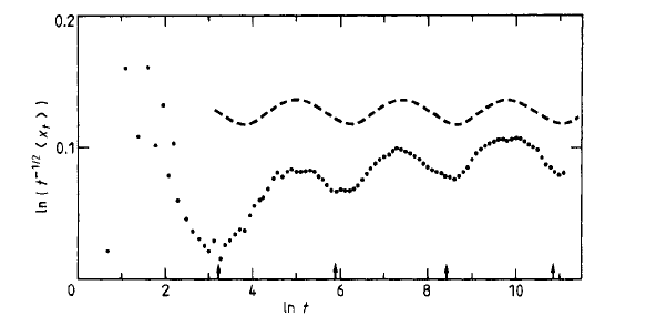
Figure 2: Temporal oscillations for the diode model, eqn (32). Here $\alpha=0.3$ and $\rho=1/0.09$, so that $\alpha\rho>1$ and $\kappa=\frac{1}{2}$. The dots represent an average of Monte Carlo simulations over $10\,000$ samples of the environment with a random walk of 200 000 steps in each realization. The broken curve refers to the exact asymptotic solution (34). The arrows indicate the simulated locations of the minima $t_{k}$, the asymptotic spacing of which is predicted to be $\ln\rho\approx 2.41$. Reproduced from Bernasconi J. and Schneider W.R. (1982) Diffusion on a one-dimensional lattice with random asymmetric transition rates. Journal of Physics A: Mathematical and General, 15, L729–L734, by permission of IOP Publishing Ltd.

In contrast, for $\alpha\rho=1$ one has

$$\operatorname{\mbox{\boldmath$E$}}_{0}X_{n}\sim\frac{n\ln\rho}{2\ln n},\quad n\to\infty,$$

and there are no oscillations of the above kind.

These results illuminate the earlier analysis of the diode model by Solomon (1975), which in the main has revealed the following. If $\alpha\rho=1$ then $X_{n}$ satisfies the strong LLN:

$$\lim_{n\to\infty}\frac{X_{n}}{n/\ln n}=\frac{\ln\rho}{2},\quad\operatorname{\mbox{\boldmath$P$}}_{0}\text{-a.s.},$$

while in the case $\alpha\rho>1$ the asymptotic behavior of $X_{n}$ is quite complicated and unusual: if $n_{i}\to\infty$ is a sequence of integers such that $\{\ln n_{i}\}\to\gamma$ (here $\{a\}=a-[a]$ denotes the fractional part of $a$), then the distribution of $n_{i}^{-\kappa}X_{n_{i}}$ under $\operatorname{\mbox{\boldmath$P$}}_{0}$ converges to a non-degenerate distribution which depends on $\gamma$. Thus, the very existence of the limiting distribution of $X_{n}$ and the limit itself heavily depend on the subsequence $n_{i}$ chosen to approach infinity.

This should be compared with a more “regular” result in Theorem 3. Note that almost all the conditions of this theorem are satisfied in the diode model, except that here the distribution of $\ln\rho_{0}$ is arithmetic (recall that the value $\ln\rho_{0}=-\infty$ is permissible), so it is the discreteness of the environment distribution that does not provide enough “mixing” and hence leads to such peculiar features of the asymptotics.

9 Some Generalizations and
Variations

Most of the results discussed above in the simplest context of RWRE with nearest-neighbor jumps in an i.i.d. random environment, have been extended to some other cases. One natural generalization is to relax the i.i.d. assumption, e.g. by considering stationary ergodic environments (see details in Zeitouni (2004)). In this context, one relies on an ergodic theorem instead of the usual strong LLN. For instance, this way one readily obtains an extension of Solomon’s criterion of transience vs. recurrence (see Theorem 1, Section 2). Other examples include an LLN (along with a formula for the asymptotic velocity, cf. Theorem 2, Section 3), a CLT and stable laws for the asymptotic distribution of $X_{n}$ (cf. Theorem 3, Section 5), and Sinai’s localization result for the recurrent RWRE (cf. Theorem 4, Section 6). Usually, however, ergodic theorems cannot be applied directly (like, e.g., to $X_{n}$, as the sequence $X_{n}-X_{n-1}$ is not stationary). In this case, one rather uses the hitting times which possess the desired stationarity (cf. Sections 3, 4). In some situations, in addition to stationarity one needs suitable mixing conditions in order to ensure enough decoupling (e.g., in Sinai’s problem). The method of environment viewed from the particle (see Section 7) is also suited very well to dealing with stationarity.

In the remainder of this section, we describe some other generalizations including RWRE with bounded jumps, RWRE where randomness is attached to bonds rather than sites, and continuous-time (symmetric) RWRE driven by the randomized master equation.

9.1 RWRE with Bounded Jumps

The previous discussion was restricted to the case of RWRE with nearest-neighbor jumps. A natural extension is RWRE with bounded jumps. Let $L,R$ be fixed natural numbers, and suppose that from each site $x\in\mathbb{Z}$ jumps are only possible to the sites $x+i$,  $i=-L,\dots,R$, with (random) probabilities

$$p_{x}(i)\geq 0,\quad\sum_{i=-L}^{R}p_{x}(i)=1.$$ (35)

We assume that the random vectors $p_{x}(\cdot)$ determining the environment are i.i.d. for different $x\in\mathbb{Z}$ (although many results can be extended to the stationary ergodic case).

The study of asymptotic properties of such a model is essentially more complex, as it involves products of certain random matrices and hence must use extensively the theory of Lyapunov exponents (see details and further references in Brémont (2004)). Lyapunov exponents, being natural analogs of logarithms of eigenvalues, characterize the asymptotic action of the product of random matrices along (random) principal directions, as described by Oseledec’s multiplicative ergodic theorem. In most situations, however, the Lyapunov spectrum can only be accessed implicitly, which makes the analysis rather hard.

To explain how random matrices arise here, let us first consider a particular case $R=1$,  $L\geq 1$. Assume that $p_{x}(-L),p_{x}(1)\geq\delta>0$ for all $x\in\mathbb{Z}$ (ellipticity condition, cf. eqn (5)), and consider the hitting probabilities $u_{n}:=\operatorname{\mathit{P}}_{n}^{\omega}\{T_{0}<\infty\}$, where $T_{0}:=\min\{t\geq 0:X_{t}\leq 0\}$ (cf. Section 2). By decomposing with respect to the first step, for $n\geq 1$ we obtain the difference equation

$$u_{n}=p_{n}(1)\,u_{n+1}+\sum_{i=0}^{L}p_{n}(-i)\,u_{n-i}$$ (36)

with the boundary conditions $u_{0}=\dots=u_{-L+1}=1$. Using that $1=p_{n}(1)+\sum_{i=0}^{L}p_{n}(-i)$, we can rewrite eqn (36) as

$$p_{n}(1)\left(u_{n}-u_{n+1}\right)=\sum_{i=1}^{L}p_{n}(-i)\left(u_{n-i}-u_{n}\right),$$

or equivalently

$$v_{n}=\sum_{i=1}^{L}b_{n}(i)\,v_{n-i},$$ (37)

where $v_{i}:=u_{i}-u_{i+1}$ and

$$b_{n}(i):=\frac{p_{n}(-i)+\dots+p_{n}(-L)}{p_{n}(1)}.$$ (38)

Recursion (37) can be written in a matrix form, $V_{n}=M_{n}V_{n-1}$, where $V_{n}:=(v_{n},\dots,v_{n-L+1})^{\top}$,

$$M_{n}:=\left(\begin{array}[]{cccc}b_{n}(1)&\dots&\dots&b_{n}(L)\\[3.60004pt] 1&\dots&0&0\\[-1.20007pt] \vdots&\ddots&\vdots&\vdots\\[1.20007pt] 0&\dots&1&0\end{array}\right),$$ (39)

and by iterations we get (cf. eqn (10))

$$V_{n}=M_{n}\cdots M_{1}V_{0},\quad V_{0}=(1-u_{1},0,\dots,0)^{\top}.$$

Note that $M_{n}$ depends only on the transition probability vector $p_{n}(\cdot)$, and hence $M_{n}\cdots M_{1}$ is the product of i.i.d. random (non-negative) matrices. ByFurstenberg-Kesten’s theorem, the limiting behavior of such a product, as $n\to\infty$, is controlled by the largest Lyapunov exponent

$$\gamma_{1}:=\lim_{n\to\infty}n^{-1}\ln\|M_{n}\dots M_{1}\|$$ (40)

(by Kingman’s sub-additive ergodic theorem, thelimit exists $\operatorname{\mathbb{P}}$-a.s. and is non-random). It follows that, $\operatorname{\mbox{\boldmath$P$}}_{0}$-a.s., the RWRE $X_{n}$ is transient if and only if $\gamma_{1}\neq 0$, and moreover, $X_{n}\to+\infty\,(-\infty$) when $\gamma_{1}<0\,(\,>0)$, whereas $\varliminf X_{n}=-\infty$, $\varlimsup X_{n}=+\infty$ when $\gamma_{1}=0$.

For orientation, note that if $p_{n}(i)=p(i)$ are non-random constants, then $\gamma_{1}=\ln\lambda_{1}$, where $\lambda_{1}>0$ is the largest eigenvalue of $M_{0}$, and so $\gamma_{1}<0$ if and only if $\lambda_{1}<1$. The latter means that the characteristic polynomial $\varphi(\lambda):=\det(M_{0}-\lambda I)$ satisfies the condition $(-1)^{L}\varphi(1)>0$. To evaluate $\det(M_{0}-I)$, replace the first column by the sum of all columns and expand to get $\varphi(1)=(-1)^{L-1}(b_{1}+\cdots+b_{L})$. Substituting expressions (38) it is easy to see that the above condition amounts to $p(1)-\sum_{i=1}^{L}i\,p(-i)>0$, that is, the mean drift of the random walk is positive and hence $X_{n}\to+\infty$ a.s.

In the general case, $L\geq 1$, $R\geq 1$, similar considerations lead to the following matrices of order $d:=L+R-1$ (cf. eqn (39))

$$M_{n}=\left(\begin{array}[]{cccccc}a_{n}(R-1)&\dots&a_{n}(1)&b_{n}(1)&\dots&b_{n}(L)\\[3.60004pt] 1&0&\dots&\dots&\dots&0\\[3.60004pt] 0&1&0&\dots&\dots&0\\[-1.20007pt] \vdots&\vdots&\ddots&\vdots&\vdots&\vdots\\[-1.20007pt] \vdots&\vdots&\vdots&\ddots&\vdots&\vdots\\[1.20007pt] 0&\dots&\dots&0&1&0\end{array}\right)$$

where $b_{n}(i)$ are given by (38) and

$$a_{n}(i):=-\frac{p_{n}(i)+\dots+p_{n}(R)}{p_{n}(R)}.$$

Suppose that the ellipticity condition is satisfied in the form $p_{n}(i)\geq\delta>0$, $i\neq 0$, $-L\leq i\leq R$, and let $\gamma_{1}\geq\gamma_{2}\geq\dots\geq\gamma_{d}$ be the (non-random) Lyapunov exponents of $\{M_{n}\}$. The largest exponent $\gamma_{1}$ is again given by eqn (40), while other exponents are determined recursively from the equalities

$$\gamma_{1}+\dots+\gamma_{k}=\lim_{n\to\infty}n^{-1}\ln\|{\wedge^{k}}(M_{n}\cdots M_{1})\|$$

($1\leq k\leq d$). Here $\wedge$ denotes the external (anti-symmetric) product: $x\wedge y=-y\wedge x$  ($x,y\in\mathbb{R}^{d}$), and $\wedge^{k}M$ acts on the external product space ${\wedge^{k}}\mathbb{R}^{d}$, generated by the canonical basis $\{e_{i_{1}}\wedge\cdots\wedge e_{i_{k}},\ 1\leq i_{1}<\cdots<i_{k}\leq d\}$, as follows:

$${\wedge^{k}}M(x_{1}\wedge\cdots\wedge x_{k}):=M(x_{1})\wedge\cdots\wedge M(x_{k}).$$

One can show that all exponents except $\gamma_{R}$ are sign definite: $\gamma_{R-1}>0>\gamma_{R+1}$. Moreover, it is the sign of $\gamma_{R}$ that determines whether the RWRE is transient or recurrent, the dichotomy being the same as in the case $R=1$ above (with $\gamma_{1}$ replaced by $\gamma_{R}$). Let us also mention that an LLN and CLT can be proved here (see Brémont (2004)).

In conclusion, let us point out an alternative approach due to Bolthausen and Goldsheid (2000) who studied a more general RWRE on a strip $\mathbb{Z}\times\{0,1,\dots,\allowbreak m-1\}$. The link between these two models is given by the representation $X_{n}=mY_{n}+Z_{n}$, where $m:=\max\{L,R\}$,  $Y_{n}\in\mathbb{Z}$,  $Z_{n}\in\{0,\dots,m-1\}$. Random matrices arising here are constructed indirectly using an auxiliary stationary sequence. Even though these matrices are non-independent, thanks to their positivity the criterion of transience can be given in terms of the sign of the largest Lyapunov exponent, which is usually much easier to deal with. An additional attractive feature of this approach is that the condition $p_{x}(R)>0$ ($\operatorname{\mathbb{P}}$-a.s.), which was essential for the previous technique, can be replaced with a more natural condition $\operatorname{\mathbb{P}}\{p_{x}(R)>0\}>0$.

9.2 Random Bonds RWRE

Instead of having random probabilities of jumps at each site, one could assign random weights to bonds between the sites. For instance, the transition probabilities $p_{x}=p(x,x+1,\omega)$ can be defined by

$$p_{x}=\frac{c_{x,x+1}}{c_{x-1,x}+c_{x,x+1}},$$ (41)

where $c_{x,x+1}>0$ are i.i.d. random variables on the environment space $\Omega$.

The difference between the two models may not seem very prominent, but the behavior of the walk in the modified model (41) appears to be quite different. Indeed, working as in Section 2 we note that

$$\rho_{x}=\frac{q_{x}}{p_{x}}=\frac{c_{x-1,x}}{c_{x,x+1}},$$

hence, exploiting formulas (11) and (41), we obtain, $\operatorname{\mathbb{P}}$-a.s.,

$$\frac{1}{1-u_{1}}=\sum_{x=0}^{n-1}\frac{c_{01}}{c_{x,x+1}}\sim c_{01}\,n\operatorname{\mathbb{E}}c_{01}^{-1}\to\infty,$$ (42)

since $\operatorname{\mathbb{E}}c_{01}^{-1}>0$. Therefore, $f_{00}=1$, i.e. the random walk is recurrent ($\operatorname{\mbox{\boldmath$P$}}_{0}$-a.s.).

The method of environment viewed from the particle can also be applied here (see Sznitman (2004)). Similarly to Section 7, we define a new probability measure $\operatorname{\mathbb{Q}}=f(\omega)\operatorname{\mathbb{P}}$ using the density

$$f(\omega)=Z^{-1}\bigl{(}c_{-1,0}(\omega)+c_{01}(\omega)\bigr{)},$$

where $Z=2\operatorname{\mathbb{E}}c_{01}$ is the normalizing constant (we assume that $\operatorname{\mathbb{E}}c_{01}<\infty$). One can check that $\operatorname{\mathbb{Q}}$ is invariant with respect to the transition kernel eqn (41), and by similar arguments as in Section 7 we obtain that $\lim_{n\to\infty}X_{n}/n$ exists ($\operatorname{\mathit{P}}_{0}^{\omega}$-a.s.) and is given by

$$\int_{\Omega}d(0,\omega)\operatorname{\mathbb{Q}}({\mathrm{d}}\omega)=Z^{-1}\operatorname{\mathbb{E}}\left[c_{01}-c_{-1,0}\right]=0,$$

so the asymptotic velocity vanishes.

Furthermore, under suitable technical conditions on the environment (e.g., $c_{01}$ being bounded away from $0$ and $\infty$, cf. eqn (5)), one can prove the following CLT:

$$\lim_{n\to\infty}\operatorname{\mbox{\boldmath$P$}}_{0}\biggl{\{}\frac{X_{n}}{\sqrt{n\sigma^{2}}}\leq x\biggr{\}}=\varPhi(x),$$ (43)

where $\sigma^{2}=\left(\operatorname{\mathbb{E}}c_{01}\cdot\operatorname{\mathbb{E}}c_{01}^{-1}\right)^{-1}$. Note that $\sigma^{2}\leq 1$ (with a strict inequality if $c_{01}$ is not reduced to a constant), which indicates some slowdown in the spatial spread of the random bonds RWRE, as compared to the ordinary symmetric random walk.

Thus, there is a dramatic distinction between the random bonds RWRE, which is recurrent and diffusive, and the random sites RWRE, with a much more complex asymptotics including both transient and recurrent scenarios, slowdown effects and subdiffusive behavior. This can be explained heuristically by noting that the random bonds RWRE is reversible, that is, $m(x)\,p(x,y)=m(y)\,p(y,x)$ for all $x,y\in\mathbb{Z}$, with $m(x):=c_{x-1,x}+c_{x,x+1}$ (this property also easily extends to multidimensional versions). Hence, it appears impossible to create extended traps which would retain the particle for a very long time. Instead, the mechanism of the diffusive slowdown in a reversible case is associated with the natural variability of the environment resulting in the occasional occurrence of isolated “screening” bonds with an anomalously small weight $c_{x,x+1}$.

Let us point out that the RWRE determined by eqn (41) can be interpreted in terms of the random conductivity model (see Hughes, 1996). Suppose that each random variable $c_{x,x+1}$ attached to the bond $(x,x+1)$ has the meaning of the conductance of this bond (the reciprocal, $c_{x,x+1}^{-1}$, being its resistance). If a voltage drop $V$ is applied across the system of $N$ successive bonds, say from $0$ to $N$, then the same current $I$ flows in each of the conductors and byOhm’s law we have $I=c_{x,x+1}V_{x,x+1}$, where $V_{x,x+1}$ is the voltage drop across the corresponding bond. Hence

$$V=\sum_{x=0}^{N}V_{x,x+1}=I\sum_{x=0}^{N}c_{x,x+1}^{-1},$$

which amounts to saying that the total resistance of the system of consecutive elements is given by the sum of the individual resistances. The effective conductivity of the finite system, $\overline{c}_{N}$, is defined as the average conductance per bond, so that

$$\overline{c}^{\,-1}_{N}=\frac{1}{N}\sum_{x=0}^{N}c_{x,x+1}^{-1},$$

and by the strong LLN, $\overline{c}_{N}^{\,-1}\to\operatorname{\mathbb{E}}c_{01}^{-1}$ as $N\to\infty$ ($\operatorname{\mathbb{P}}$-a.s.). Therefore, the effective conductivity of the infinite system is given by $\overline{c}=\left(\operatorname{\mathbb{E}}c_{01}^{-1}\right)^{-1}$, and we note that $\overline{c}<\operatorname{\mathbb{E}}c_{01}$ if the random medium is non-degenerate.

Returning to the random bonds RWRE, eqn (41), it is easy to see that a site $j$ is recurrent if and only if the conductance $c_{j,\infty}$ between $x$ and $\infty$ equals zero. Using again Ohm’s law, we have (cf. eqn (42))

$$c^{-1}_{j,+\infty}=\sum_{x=j}^{\infty}c_{x,x+1}^{-1}=\infty,\quad\operatorname{\mathbb{P}}\text{-a.s.}$$

and we recover the result about recurrence.

9.3 Continuous-Time RWRE

As in the discrete-time case, a random walk on $\mathbb{Z}$ with continuous time is a homogeneous Markov chain $X_{t}$, $t\in[0,\infty)$, with state space $\mathbb{Z}$ and nearest neighbor (or at least bounded) jumps. The term “Markov” as usual refers to the “lack of memory” property, which amounts to saying that from the entire history of the process development up to a given time, only the current position of the walk is important for the future evolution while all other information is irrelevant.

Since there is no smallest time unit as in the discrete-time case, it is convenient to describe transitions of $X_{t}$ in terms of transition rates characterizing the likelihood of various jumps during a very short time. More precisely, if $p_{xy}(t):=P\{X_{t}=y\,|\,X_{0}=x\}$ are the transition probabilities over time $t$, then for $h\to 0$

$$p_{xy}(h) =c_{xy}h+o(h)\qquad(x\neq y),$$ (44)

$$p_{xx}(h) =1-h\sum_{y\neq x}c_{xy}+o(h).$$

Equations for the functions $p_{xy}(t)$ can then be derived by adapting the method of decomposition commonly used for discrete-time Markov chains (cf. Section 2). Here it is more convenient to decompose with respect to the “last” step, i.e. by considering all possible transitions during a small increment of time at the end of the time interval $[0,t+h]$. Using Markov property and eqn (44) we can write

$$p_{0x}(t+h) =h\sum_{y\neq x}p_{0y}(t)\,c_{yx}$$

$$+p_{0x}(t)\biggl{(}1-h\sum_{y\neq x}c_{xy}\biggr{)}+o(h),$$

which in the limit $h\to 0$ yields the master equation (or Chapman-Kolmogorov’s forward equation)

$$\frac{{\mathrm{d}}}{{\mathrm{d}}t}p_{0x}(t)=\sum_{y\neq x}\bigl{\{}c_{yx}p_{0y}(t)-c_{xy}p_{0x}(t)\bigr{\}},$$ (45)

$$p_{0x}(0)=\delta_{0}(x),$$

where $\delta_{0}(x)$ is the Kronecker symbol.

Continuous-time RWRE are therefore naturally described via the randomized master equation, i.e. with random transition rates. The canonical example, originally motivated by Dyson’s study of the chain of harmonic oscillators with random couplings, is a symmetric nearest-neighbor RWRE, where the random transition rates $c_{xy}$ are non-zero only for $y=x\pm 1$ and satisfy the condition $c_{x,x+1}=c_{x+1,x}$, otherwise being i.i.d. (see Alexander et al. (1981)). In this case, the problem (45) can be formally solved using the Laplace transform, leading to the equations

$$s+G^{+}_{0}+G^{-}_{0} =[\hat{p}_{0}(s)]^{-1},$$ (46)

$$s+G^{-}_{x}+G^{+}_{x} =0\quad(x\neq 0),$$ (47)

where $G^{-}_{x}$, $G^{+}_{x}$ are defined as

$$G^{\pm}_{x}:=c_{x,x\pm 1}\,\frac{\hat{p}_{0x}(s)-\hat{p}_{0,x\pm 1}(s)}{\hat{p}_{0x}(s)}$$ (48)

and $\hat{p}_{0x}(s):=\int_{0}^{\infty}p_{0x}(t)\,{\mathrm{e}}^{-st}\,{\mathrm{d}}t$. From eqs (47), (48) one obtains the recursion

$$G^{\pm}_{x} =\biggl{(}\frac{1}{c_{x,x\pm 1}}+\frac{1}{s+G_{x\pm 1}^{+}}\biggr{)}^{-1},$$ (49)

$$x =0,\pm 1,\pm 2,\dots$$

The quantities $G^{\pm}_{0}$ are therefore expressed as infinite continued fractions depending on $s$ and the random variables $c_{x,x\pm 1}$, $c_{x,x\pm 2}$, …The function $\hat{p}_{00}(s)$ can then be found from eqn (46).

In its generality, the problem is far too hard, and we shall only comment on how one can evaluate the annealed mean

$$\operatorname{\mathbb{E}}\hat{p}_{00}(s)=\operatorname{\mathbb{E}}(s+G^{+}_{0}+G^{-}_{0})^{-1}.$$

According to eqn (49), the random variables $G^{+}_{0}$, $G^{-}_{0}$ are determined by the same algebraic formula, but involve the rate coefficients from different sides of site $x$, and hence are i.i.d. Furthermore, eqn (49) implies that the random variables $G^{+}_{0}$, $G^{+}_{1}$ have the same distribution and, moreover, $G^{+}_{1}$ and $c_{01}$ are independent. Therefore, eqn (49) may be used as an integral equation for the unknown density function of $G^{+}_{0}$. It can be proved that the suitable solution exists and is unique, and although an explicit solution is not available, one can obtain the asymptotics of small values of $s$, thereby rendering information about the behavior of $p_{00}(t)$ for large $t$. More specifically, one can show that if $c_{*}:=\bigl{(}\operatorname{\mathbb{E}}c_{01}^{-1}\bigr{)}^{-1}>0$ then

$$\operatorname{\mathbb{E}}\hat{p}_{00}(s)\sim(4c_{*}s)^{-1/2},\quad s\to 0,$$

and so by a Tauberian theorem

$$\operatorname{\mathbb{E}}p_{00}(t)\sim(4\pi c_{*}t)^{-1/2},\quad t\to\infty.$$ (50)

Note that asymptotics (50) appears to be the same as for an ordinary symmetric random walk with constant transition rates $c_{x,x+1}=c_{x+1,x}=c_{*}$, suggesting that the latter provides an “effective medium approximation” (EMA) for the RWRE considered above.

This is further confirmed by the asymptotic calculation of the annealed mean-square displacement, $\operatorname{\mbox{\boldmath$E$}}_{0}X_{t}^{2}\sim 2c_{*}t$ as $t\to\infty$ (Alexander et al. 1981). Moreover, Kawazu and Kesten (1984) proved that $X_{t}$ is asymptotically normal:

$$\lim_{t\to\infty}\operatorname{\mbox{\boldmath$P$}}_{0}\biggl{\{}\frac{X_{t}}{\sqrt{2c_{*}t}}\leq x\biggr{\}}=\varPhi(x).$$ (51)

Therefore, if $c_{*}>0$ then the RWRE has the same diffusive behavior as the corresponding ordered system, with a well-defined diffusion constant $D=c_{*}$.

In the case where $c_{*}=0$ (i.e., $\operatorname{\mathbb{E}}c_{01}^{-1}=\infty$), one may expect that the RWRE exhibits subdiffusive behavior. For example, if the density function of the transition rates is modelled by

$$f_{a}(u)=(1-\alpha)\,u^{-\alpha}{\mathbf{1}}_{\{0<u<1\}}\quad(0<\alpha<1),$$

then, as shown by Alexander et al. (1981),

$$\operatorname{\mathbb{E}}p_{00}(t) \sim C_{\alpha}\,t^{-(1-\alpha)/(2-\alpha)},$$

$$\operatorname{\mbox{\boldmath$E$}}_{0}X_{t}^{2} \sim C^{\prime}_{\alpha}\,t^{2(1-\alpha)/(2-\alpha)}.$$

In fact, Kawazu and Kesten (1984) proved that in this case $t^{-\alpha/(1+\alpha)}X_{t}$ has a (non-Gaussian) limit distribution as $t\to\infty$.

To conclude the discussion of the continuous-time case, let us point out that some useful information about recurrence of $X_{t}$ can be obtained by considering an imbedded (discrete-time) random walk $\tilde{X}_{n}$, defined as the position of $X_{t}$ after $n$ jumps. Note that continuous-time Markov chains admit an alternative description of their evolution in terms of sojourn times and the distribution of transitions at a jump. Namely, if the environment $\omega$ is fixed then the random sojourn time of $X_{t}$ in each state $x$ is exponentially distributed with mean $1/c_{x}$, where $c_{x}:=\sum_{y\neq x}c_{xy}$, while the distribution of transitions from $x$ is given by the probabilities $p_{xy}=c_{xy}/c_{x}$.

For the symmetric nearest-neighbor RWRE considered above, the transition probabilities of the imbedded random walk are given by

$$p_{x}:=p_{x,x+1} =\frac{c_{x,x+1}}{c_{x-1,x}+c_{x,x+1}},$$

$$q_{x}:=p_{x,x-1} =1-p_{x},$$

and we recognize here the transition law of a random walk in the random bonds environment considered in Section 9.2 (cf. eqn (41)). Recurrence and zero asymptotic velocity established there are consistent with the results discussed in the present section (e.g., note that the CLT for both $X_{n}$, eqn (43), and $X_{t}$, eqn (51), does not involve any centering). Let us point out, however, that a “naive” discretization of time using the mean sojourn time appears to be incorrect, as this would lead to the scaling $t=n\delta_{1}$ with $\delta_{1}:=\operatorname{\mathbb{E}}(c_{-1,0}+c_{01})^{-1}$, while from comparing the limit theorems in these two cases, one can conclude that the true value of the effective discretization step is given by $\delta_{*}:=(2c_{*})^{-1}=\frac{1}{2}\operatorname{\mathbb{E}}c_{01}^{-1}$. In fact, by the arithmetic-harmonic mean inequality we have $\delta_{*}>\delta_{1}$, which is a manifestation of the RWRE’s diffusive slowdown.

10 RWRE in Higher Dimensions

Multidimensional RWRE with nearest-neighborjumps are defined in a similar fashion: from site $x\in\mathbb{Z}^{d}$ the random walk can jump to one of the $2d$ adjacent sites $x+e\in\mathbb{Z}^{d}$ (such that $|e|=1$), with probabilities $p_{x}(e)\geq 0$,  $\sum_{|e|=1}p_{x}(e)=1$, where the random vectors $p_{x}(\cdot)$ are assumed to be i.i.d. for different $x\in\mathbb{Z}^{d}$. As usual, we will also impose the condition of uniform ellipticity:

$$p_{x}(e)\geq\delta>0,\quad|e|=1,\ \ x\in\mathbb{Z}^{d},\ \,\operatorname{\mathbb{P}}\text{-a.s.}.$$ (52)

In contrast to the one-dimensional case, theory of RWRE in higher dimensions is far from maturity. Possible asymptotic behaviors of the RWRE for $d\geq 2$ are not understood well enough, and many basic questions remain open. For instance, no definitive classification of the RWRE is available regarding transience and recurrence. Similarly, LLN and CLT have been proved only for a limited number of specific models, while no general sharp results have been obtained. On a more positive note, there has been considerable progress in recent years in the so-called ballistic case, where powerful techniques have been developed (see Sznitman (2002, 2004) and Zeitouni (2003, 2004)). Unfortunately, not much is known for non-ballistic RWRE, apart from special cases of balanced RWRE in $d\geq 2$ (Lawler 1982), small isotropic perturbations of ordinary symmetric random walks in $d\geq 3$ (Bricmont and Kupiainen 1991), and some examples based on combining components of ordinary random walks and RWRE in $d\geq 7$ (Bolthausen et al. 2003). In particular, there are no examples of subdiffusive behavior in any dimension $d\geq 2$, and in fact it is largely believed that a CLT is always true in any uniformly elliptic, i.i.d. random environment in dimensions $d\geq 3$, with somewhat less certainty about $d=2$. A heuristic explanation for such a striking difference with the case $d=1$ is that due to a less restricted topology of space in higher dimensions, it is much harder to force the random walk to visit traps, and hence the slowdown is not so pronounced.

In what follows, we give a brief account of some of the known results and methods in this fast developing area (for further information and specific references, see an extensive review by Zeitouni (2004)).

10.1 Zero-One Laws and LLNs

A natural first step in a multidimensional context is to explore the behavior of the random walk $X_{n}$ as projected on various one-dimensional straight lines. Let us fix a test unit vector $\ell\in\mathbb{R}^{d}$, and consider the process $Z_{n}^{\ell}:=X_{n}\cdot\ell$. Then for the events $A_{\pm\ell}:=\{\lim_{n\to\infty}Z^{\ell}_{n}=\pm\infty\}$ one can show that

$$\operatorname{\mbox{\boldmath$P$}}_{0}(A_{\ell}\cup A_{-\ell})\in\{0,1\}.$$ (53)

That is to say, for each $\ell$ the probability that the random walk escapes to infinity in the direction $\ell$ is either $0$ or $1$.

Let us sketch the proof. We say that $\tau$ is record time if $|Z^{\ell}_{t}|>|Z^{\ell}_{k}|$ for all $k<t$, and regeneration time if in addition $|Z^{\ell}_{\tau}|\leq|Z^{\ell}_{n}|$ for all $n\geq\tau$. Note that by the ellipticity condition (52), $\varlimsup_{n\to\infty}|Z^{\ell}_{n}|=\infty$ ($\operatorname{\mbox{\boldmath$P$}}_{0}$-a.s.), hence there is an infinite sequence of record times $0=\tau_{0}<\tau_{1}<\tau_{2}<\cdots$ If $\operatorname{\mbox{\boldmath$P$}}_{0}(A_{\ell}\cup A_{-\ell})>0$, we can pick a subsequence of record times $\tau^{\prime}_{i}$, each of which has a positive $\operatorname{\mbox{\boldmath$P$}}_{0}$-probability to be a regeneration time (because otherwise $|Z^{\ell}_{n}|$ would persistently backtrack towards the origin and the event $A_{\ell}\cup A_{-\ell}$ could not occur). Since the trials for different record times are independent, it follows that a regeneration time $\tau^{*}$ occurs $\operatorname{\mbox{\boldmath$P$}}_{0}$-a.s. Repeating this argument, we conclude that there exists an infinite sequence of regeneration times $\tau_{i}^{*}$, which implies that $|Z^{\ell}_{n}|\to\infty$ ($\operatorname{\mbox{\boldmath$P$}}_{0}$-a.s.), i.e., ${\operatorname{\mbox{\boldmath$P$}}(A_{\ell}\cup A_{-\ell})=1}$.

Regeneration structure introduced by the sequence $\{\tau_{i}^{*}\}$ plays a key role in further analysis of the RWRE and is particularly useful for proving an LLN and a CLT, due to the fact that pieces of the random walk between consecutive regeneration times (and fragments of the random environment involved thereby) are independent and identically distributed (at least starting from $\tau_{1}^{*}$). In this vein, one can prove a “directional” version of the LLN, stating that for each $\ell$ there exist deterministic $v_{\ell},v_{-\ell}$ (possibly zero) such that

$$\lim_{n\to\infty}\frac{Z_{n}^{\ell}}{n}=v_{\ell}\,{\mathbf{1}}_{A_{\ell}}+v_{-\ell}\,{\mathbf{1}}_{A_{-\ell}},\quad\operatorname{\mbox{\boldmath$P$}}_{0}\text{-a.s.}$$ (54)

Note that if $\operatorname{\mbox{\boldmath$P$}}_{0}(A_{\ell})\in\{0,1\}$, eqn (54) in conjunction with eqn (53) would readily imply

$$\lim_{n\to\infty}\frac{Z_{n}^{\ell}}{n}=v_{\ell},\quad\operatorname{\mbox{\boldmath$P$}}_{0}\text{-a.s.}$$ (55)

Moreover, if $\operatorname{\mbox{\boldmath$P$}}_{0}(A_{\ell})\in\{0,1\}$ for any $\ell$, then there exists a deterministic $v$ (possibly zero) such that

$$\lim_{n\to\infty}\frac{X_{n}}{n}=v,\quad\operatorname{\mbox{\boldmath$P$}}_{0}\text{-a.s.}$$ (56)

Therefore, it is natural to ask if a zero-one law (53) can be enhanced to that for the individual probabilities $\operatorname{\mbox{\boldmath$P$}}_{0}(A_{\ell})$. It is known that the answer is affirmative for i.i.d. environments in $d=2$, where indeed $\operatorname{\mbox{\boldmath$P$}}(A_{\ell})\in\{0,1\}$ for any $\ell$, with counter-examples in certain stationary ergodic (but not uniformly elliptic) environments. However, in the case $d\geq 3$ this is an open problem.

10.2 Kalikow’s Condition and Sznitman’s
Condition ($\mathbf{T}^{\prime}$)

An RWRE is called ballistic (ballistic in direction $\ell$) if $v\neq 0$ ($v_{\ell}\neq 0$), see eqs (55), (56). In this section, we describe conditions on the random environment which ensure that the RWRE is ballistic.

Let $U$ be a connected strict subset of $\mathbb{Z}^{d}$ containing the origin. For $x\in U$, denote by

$$g(x,\omega):=\operatorname{\mathit{E}}^{\omega}_{0}\sum_{n=0}^{T_{U}}\mathbf{1}_{\{X_{n}=x\}}$$

the quenched mean number of visits to $x$ prior to the exit time $T_{U}:=\min\{n\geq 0:X_{n}\notin U\}$. Consider an auxiliary Markov chain $\widehat{X}_{n}$, which starts from $0$, makes nearest-neighbor jumps while in $U$, with (non-random) probabilities

$$\widehat{p}_{x}(e) =\frac{\operatorname{\mathbb{E}}\left[g(x,\omega)p_{x}(e)\right]}{\operatorname{\mathbb{E}}\left[g(x,\omega)\right]},\quad x\in U,$$ (57)

and is absorbed as soon as it first leaves $U$. Note that the expectations in eqn (57) are finite; indeed, if $\alpha_{x}$ is the probability to return to $x$ before leaving $U$, then, by the Markov property, the mean number of returns is given by

$$\sum_{k=1}^{\infty}k\alpha_{x}^{k}(1-\alpha_{x})=\frac{\alpha_{x}}{1-\alpha_{x}}<\infty,$$

since, due to ellipticity, $\alpha_{x}<1$.

An important property, highlighting the usefulness of $\widehat{X}_{n}$, is that if $\widehat{X}_{n}$ leaves $U$ with probability $1$, then the same is true for the original RWRE $X_{n}$ (under the annealed law $\operatorname{\mbox{\boldmath$P$}}_{0}$), and moreover, the exit points $\widehat{X}_{{\widehat{T}}_{U}}$ and $X_{T_{U}}$ have the same distribution laws.

Let $\ell\in\mathbb{R}^{d}$, $|\ell|=1$. One says that Kalikow’s condition with respect to $\ell$ holds if the local drift of $\widehat{X}_{n}$ in the direction $\ell$ is uniformly bounded away from zero:

$$\inf_{U}\inf_{x\in U}\sum_{|e|=1}(e\cdot\ell)\,\widehat{p}_{x}(e)>0.$$ (58)

A sufficient condition for (58) is, for example, that for some $\kappa>0$

$$\operatorname{\mathbb{E}}\left[(d(0,\omega)\cdot\ell)_{+}\right]\geq\kappa\operatorname{\mathbb{E}}\left[(d(0,\omega)\cdot\ell)_{-}\right],$$

where $d(0,\omega)=\operatorname{\mathit{E}}_{0}^{\omega}X_{1}$ and $u_{\pm}:=\max\{\pm u,0\}$.

A natural implication of Kalikow’s condition (58) is that $\operatorname{\mbox{\boldmath$P$}}_{0}(A_{\ell})=1$ and $v_{\ell}>0$ (see eqn (55)). Moreover, noting that eqn (58) also holds for all $\ell^{\prime}$ in a vicinity of $\ell$ and applying the above result with $d$ non-collinear vectors from that vicinity, we conclude that under Kalikow’s condition there exists a deterministic $v\neq 0$ such that $X_{n}/n\to v$ as $n\to\infty$ ($\operatorname{\mbox{\boldmath$P$}}_{0}$-a.s.). Furthermore, it can be proved that $(X_{n}-nv)/\sqrt{n}$ converges in law to a Gaussian distribution (see Sznitman (2004)).

It is not hard to check that in dimension $d=1$ Kalikow’s condition is equivalent to $v\neq 0$ and therefore characterizes completely all ballistic walks. For $d\geq 2$, the situation is less clear; for instance, it is not known if there exist RWRE with $\operatorname{\mbox{\boldmath$P$}}(A_{\ell})>0$ and $v_{\ell}=0$ (of course, such RWRE cannot satisfy Kalikow’s condition).

Sznitman (2004) has proposed a more complicated transience condition ($\text{T}^{\prime}$) involving certain regeneration times $\tau_{i}^{*}$ similar to those described in Section 10.1. An RWRE is said to satisfy Sznitman’s condition ($\text{T}^{\prime}$) relative to direction $\ell$ if $\operatorname{\mbox{\boldmath$P$}}_{0}(A_{\ell})=1$ and for some $c>0$ and all $0<\gamma<1$

$$\operatorname{\mbox{\boldmath$E$}}_{0}\exp\Bigl{(}c\sup_{n\leq\tau_{1}^{*}}|X_{n}|^{\gamma}\Bigr{)}<\infty.$$ (59)

This condition provides a powerful control over $\tau_{1}^{*}$ for $d\geq 2$ and in particular ensures that $\tau_{1}^{*}$ has finite moments of any order. This is in sharp contrast with the one-dimensional case, and should be viewed as a reflection of much weaker traps in dimensions $d\geq 2$. Condition (59) can also be reformulated in terms of the exit distribution of the RWRE from infinite thick slabs “orthonormal” to directions $\ell^{\prime}$ sufficiently close to $\ell$. As it stands, the latter reformulation is difficult to check, but Sznitman (2004) has developed a remarkable “effective” criterion reducing the job to a similar condition in finite boxes, which is much more tractable and can be checked in a number of cases.

In fact, condition ($\text{T}^{\prime}$) follows from Kalikow’s condition, but not the other way around. In the one-dimensional case, condition ($\text{T}^{\prime}$) (applied to $\ell=1$ and $\ell=-1$) proves to be equivalent to the transient behavior of the RWRE, which, as we have seen in Theorem 2 (Section 3), may happen with $v=0$, i.e. in a non-ballistic scenario. The situation in $d\geq 2$ is quite different, as condition ($\text{T}^{\prime}$) implies that the RWRE is ballistic in the direction $\ell$ (with $v_{\ell}>0$) and satisfies a CLT (under $\operatorname{\mbox{\boldmath$P$}}_{0}$). It is not known whether the ballistic behavior for $d\geq 2$ is completely characterized by condition ($\text{T}^{\prime}$), although this is expected to be true.

10.3 Balanced RWRE

In this section we discuss a particular case of non-ballistic RWRE, for which LLN and CLT can be proved. Following Lawler (1982), we say that an RWRE is balanced if $p_{x}(e)=p_{x}(-e)$ for all $x\in\mathbb{Z}^{d}$, $|e|=1$ ($\operatorname{\mathbb{P}}$-a.s.). In this case, the local drift vanishes, $d(x,\omega)=0$, hence the coordinate processes $X_{n}^{i}$ ($i=1,\dots,d$) are martingales with respect to the natural filtration $\mathcal{F}_{n}=\sigma\{X_{0},\dots,X_{n}\}$. The quenched covariance matrix of the increments $\Delta X^{i}_{n}:=X_{n+1}^{i}-X_{n}^{i}$ ($i=1,\dots,d$) is given by

$$\operatorname{\mathit{E}}_{0}^{\omega}\left[\Delta X_{n}^{i}\,\Delta X_{n}^{j}\,|\,\mathcal{F}_{n}\right]=2\delta_{ij}p_{X_{n}}(e_{i}).$$ (60)

Since the right-hand side of eqn (60) is uniformly bounded, it follows that $X_{n}/n\to 0$ ($\operatorname{\mbox{\boldmath$P$}}_{0}$-a.s.). Further, it can be proved that there exist deterministic positive constants $a_{1},\dots,a_{d}$ such that for $i=1,\dots,d$

$$\lim_{n\to\infty}\frac{1}{n}\sum_{k=0}^{n-1}p_{X_{k}}(e_{i})=\frac{a_{i}}{2},\quad\operatorname{\mbox{\boldmath$P$}}_{0}\text{-a.s.}$$ (61)

Once this is proved, a multidimensional CLT for martingale differences yields that $X_{n}/\sqrt{n}$ converges in law to a Gaussian distribution with zero mean and the covariances $b_{ij}=\delta_{ij}a_{i}$.

The proof of (61) employs the method of environment viewed from the particle (cf. Section 7). Namely, define a Markov chain $\omega_{n}:=\theta^{X_{n}}\omega$ with the transition kernel

$$T(\omega,{\mathrm{d}}\omega^{\prime})=\sum_{i=1}^{d}\bigl{[} p_{0}(e_{i})\,\delta_{\theta\omega}({\mathrm{d}}\omega^{\prime})$$

$$+p_{0}(-e_{i})\,\delta_{\theta^{-1}\omega}({\mathrm{d}}\omega^{\prime})\bigr{]}$$

(cf. eqn (27)). The next step is to find a probability measure $\operatorname{\mathbb{Q}}$ on $\Omega$ invariant under $T$ and absolutely continuous with respect to $\operatorname{\mathbb{P}}$. Unlike the one-dimensional case, however, an explicit form of $\operatorname{\mathbb{Q}}$ is not available, and $\operatorname{\mathbb{Q}}$ is constructed indirectly as the limit of invariant measures of certain periodic modifications of the RWRE. Birkhoff’s ergodic theorem then yields, $\operatorname{\mbox{\boldmath$P$}}_{0}$-a.s.,

$$\frac{1}{n}\sum_{k=0}^{n-1}p_{X_{k}}(e_{i},\omega) =\frac{1}{n}\sum_{k=0}^{n-1}p_{0}(e_{i},\omega_{k})$$

$$\to\int_{\Omega}p_{0}(e_{i},\omega_{1})\operatorname{\mathbb{Q}}({\mathrm{d}}\omega)\geq\delta,$$

by the ellipticity condition (52), and eqn (61) follows.

With regard to transience, balanced RWRE admit a complete and simple classification. Namely, it has been proved (see Zeitouni (2004)) that any balanced RWRE is transient for $d\geq 3$ and recurrent for $d=2$ ($\operatorname{\mbox{\boldmath$P$}}_{0}$-a.s.). It is interesting to note, however, that these answers may be false for certain balanced random walks in a fixed environment ($\operatorname{\mathbb{P}}$-probability of such environments being zero, of course). Indeed, examples can be constructed of balanced random walks in $\mathbb{Z}^{2}$ and in $\mathbb{Z}^{d}$ with $d\geq 3$, which are transient and recurrent, respectively (Zeitouni 2004).

10.4 RWRE Based on Modification of
Ordinary Random Walks

A number of partial results are known for RWRE constructed on the basis of ordinary random walks via certain randomization of the environment. A natural model is obtained by a small perturbation of a simple symmetric random walk. To be more precise, suppose that: (a) $|p_{x}(e)-\frac{1}{2d}|<\varepsilon$ for all $x\in\mathbb{Z}^{d}$ and any $|e|=1$, where $\varepsilon>0$ is small enough; (b) $\operatorname{\mathbb{E}}p_{x}(e)=\frac{1}{2d}$; (c) vectors $p_{x}(\cdot)$ are i.i.d. for different $x\in\mathbb{Z}^{d}$, and (d) the distribution of the vector $p_{x}(\cdot)$ is isotropic, i.e. invariant with respect to permutations of its coordinates. Then for $d\geq 3$ Bricmont and Kupiainen (1991) have proved an LLN (with zero asymptotic velocity) and a quenched CLT (with non-degenerate covariance matrix). The proof is based on the renormalization group method, which involves decimation in time combined with a suitable spatial-temporal scaling. This transformation replaces an RWRE by another RWRE with weaker randomness, and it can be shown that iterations converge to a Gaussian fixed point.

Another class of examples are also built using small perturbations of simple symmetric random walks, but are anisotropic and exhibit ballistic behavior, providing that the annealed local drift in some direction is strong enough (see Sznitman (2004)). More precisely, suppose that $d\geq 3$ and $\eta\in(0,1)$. Then there exists $\varepsilon_{0}=\varepsilon_{0}(d,\eta)>0$ such that if $|p_{x}(e)-\frac{1}{2d}|<\varepsilon$  ($x\in\mathbb{Z}^{d}$, $|e|=1$) with $0<\varepsilon<\varepsilon_{0}$, and for some $e_{0}$ one has $\operatorname{\mathbb{E}}{}[d(x,\omega)\cdot e_{0}]\geq\varepsilon^{2.5-\eta}$ ($d=3$) or $\geq\varepsilon^{3-\eta}$ ($d\geq 4$), then Sznitman’s condition ($\text{T}^{\prime}$) is satisfied with respect to $e_{0}$ and therefore the RWRE is ballistic in the direction $e_{0}$ (cf. Section 10.2).

Examples of a different type are constructed in dimensions $d\geq 6$ by letting the first $d_{1}\geq 5$ coordinates of the RWRE $X_{n}$ behave according to an ordinary random walk, while the remaining $d_{2}=d-d_{1}$ coordinates are exposed to a random environment (see Bolthausen et al. (2003)). One can show that there exists a deterministic $v$ (possibly zero) such that $X_{n}/n\to v$ ($\operatorname{\mbox{\boldmath$P$}}_{0}$-a.s.). Moreover, if $d_{1}\geq 13$ then $(X_{n}-nv)/\sqrt{n}$ satisfies both quenched and annealed CLT. Incidentally, such models can be used to demonstrate the surprising features of the multidimensional RWRE. For instance, for $d\geq 7$ one can construct an RWRE $X_{n}$ such that the annealed local drift does not vanish, $\operatorname{\mathbb{E}}d(x,\omega)\neq 0$, but the asymptotic velocity is zero, $X_{n}/n\to 0$ ($\operatorname{\mbox{\boldmath$P$}}_{0}$-a.s.), and furthermore, if $d\geq 15$ then in this example $X_{n}/\sqrt{n}$ satisfies a quenched CLT. (In fact, one can construct such RWRE as small perturbations of a simple symmetric walk.) On the other hand, there exist examples (in high enough dimensions) where the walk is ballistic with a velocity which has an opposite direction to the annealed drift $\operatorname{\mathbb{E}}d(x,\omega)\neq 0$. These striking examples provide “experimental” evidence of many unusual properties of the multidimensional RWRE, which, no doubt, will be discovered in the years to come.

See also:  Averaging Methods; Growth Processes in Random Matrix Theory; Lagrangian Dispersion(Passive Scalar); Random Dynamical Systems; Random Matrix Theory in Physics; Stochastic Differential Equations; Stochastic Loewner Evolutions.