Electric field of a pointlike charge in a strong magnetic field and ground state of a hydrogenlike atom

Abstract

In an external constant magnetic field, so strong that the electron Larmour length is much shorter than its Compton length, we consider the modification of the Coulomb potential of a point charge owing to the vacuum polarization. We establish a short-range component of the static interaction in the Larmour scale, expressed as a Yukawa-like law, and reveal the corresponding ”photon mass” parameter. The electrostatic force regains its long-range character in the Compton scale: the tail of the potential follows an anisotropic Coulomb law, decreasing away from the charge slower along the magnetic field and faster across. In the infinite-magnetic-field limit the potential is confined to an infinitely thin string passing though the charge parallel to the external field. This is the first evidence for dimensional reduction in the photon sector of quantum electrodynamics. The one-dimensional form of the potential on the string is derived that includes a $\delta$-function centered in the charge. The nonrelativistic ground-state energy of a hydrogenlike atom is found with its use and shown not to be infinite in the infinite-field limit, contrary to what was commonly accepted before, when the vacuum polarization had been ignored. These results may be useful for studying properties of matter at the surface of extremely magnetized neutron stars.

I Introduction

The fact that the vacuum, in which an external magnetic field is present, is an optically anisotropic medium, has been known, perhaps, since the time when the nonlinearity of quantum electrodynamics was first recognized: in a nonlinear theory electromagnetic fields do interact with one another, provided that the strength of at least one of them is of the order of or larger than the characteristic value $B_{0}=m^{2}/e\simeq 4.4\times 10^{13}$G, where $m$ and $e$ are electron mass and charge, respectively. [Henceforth, we set $\hbar=c=1$ and refer to the Heaviside-Lorentz system of units.] If the external field is strong, other fields interact with it, the result of the interaction depending upon the direction specified by the external field, hence the anisotropy. Depending on the wave amplitude, the electromagnetic waves propagation in this medium may be considered as a nonlinear process bialyniska , including the transformation of one photon into two adler or more photons, or taken in the linear approximation with respect to the amplitude. In the latter case, the second-rank polarization tensor is responsible for the properties of the medium. In the kinematic domain where the photon absorption processes like electron-positron pair creation are not allowed, the polarization tensor is symmetric and real, and the medium is transparent and birefringent footnote . In the absorption domain the medium is dichroic heyl . The limit of low frequency and momentum belongs to the transparency domain and corresponds to a constant anisotropic dielectric permeability of the medium. In this limit the polarization tensor may be obtained by differentiations with respect to the fields of an effective Lagrangian, calculated on the class of constant external electric and magnetic fields. For small values of these fields blp and for extremely large heyl fields the polarization operator was in this way considered using the effective Lagrangian of Heisenberg-Euler calculated euler within the one-loop approximation. (The two-loop calculations are also available lebedev .) The knowledge of this limit is useful for studying the dielectric screening of the fields that are (almost) static and (almost) constant in space. For more general purposes, however, this limit is not sufficient, and one should calculate the polarization tensor directly, using the Feynman diagram technique of the Furry picture in the external magnetic field. On the photon mass shell, i.e. when the photon energy, $k_{0}$, and 3-momentum, $\bf k$, are related by the free vacuum dispersion law $k_{0}^{2}={\bf k}^{2},$ such calculations were done by Adler adler2 and Constantinescu constantinescu . The results obtained are appropriate for handling the photon propagation in weakly dispersive medium, when the dispersion law does not essentially deviate from its vacuum shape. The polarization operator for the case of general relation between the photon mass and momentum was calculated by Batalin and Shabad batalin , Tsai tsai , Baier et al. baier , and Melrose and Stoneham melrose1 . This gave the possibility of studying the photon propagation annphys under the conditions where the deviation from the vacuum dispersion law may be very strong either due to the phenomenon of the cyclotron resonance in the vacuum polarization nuovcimlet - this phenomenon is responsible for the effect of photon capture by a magnetic field nature ; ShUs ; wunner - or due to magnetic fields, much larger than $B_{0}$ kratkie ; shabtrudy ; mikheev ; japan , or due to the both circumstances (see Ref. zhetf where the photon capture effect was extended to low frequencies for extra-large fields).

Although much work has been devoted to study of electromagnetic wave propagation in the magnetized vacuum, problems of electro- and magneto-statics in this medium did not attract sufficient attention, save Refs. loskutov1 ; skobelev , where corrections to the Coulomb law were found when these are small: for $B/B_{0}\ll 1$ in loskutov1 , or at large distances from the source for $1\ll B/B_{0}\ll 3\pi\alpha^{-1}$ in skobelev , where $\alpha=e^{2}/4\pi=1/137$ in the fine-structure constant. Here we proceed with an investigation of some electrostatics in the presence of a strong external magnetic field in the vacuum to find that for sufficiently large $b\equiv B/B_{0}\gg 1$ the electric field produced by a pointlike charge at rest may be significantly modified by the vacuum polarization, the modification being determined by the characteristic factor $\alpha b$. We note first of all that expressions for the dielectric permeability of the magnetized vacuum obtained from the Heisenberg-Euler Lagrangian are applicable only as far as the fields slowly varying in the space are concerned. Otherwise, the spatial dispersion becomes important. For this reason, when considering the electric field produced by a pointlike electric charge in the present paper, we address again to the polarization tensor calculated off-shell in batalin ; tsai ; baier ; melrose1 ; annphys , taking it in the static limit $k_{0}=0$, but keeping the dependence on $\bf k$. The corresponding spatial dispersion effects will be essential for getting some important features of the modified Coulomb potential.

Using the tensor decomposition of the polarization operator and the photon Green function, established in batalin ; annphys in an approximation-independent way, we find that photons of only one polarization mode (mode-2 in the nomenclature of these references, see below) may be carriers of electrostatic force. This is in agreement with the fact that the electromagnetic field of these photons is, in the static limit, purely electric and longitudinal. The photons of the other two modes mediate in this limit the magneto-static field of constant currents.

In magnetic fields $B\gg B_{0}$, which we are dealing with when describing the static field, produced in the magnetized vacuum by a point electric charge, the electron Larmour length $L_{\rm B}\equiv(eB)^{-1/2}=\lambda_{\rm C}b^{-1/2}$ is much less than the electron Compton length $\lambda_{\rm C}=m^{-1}$. Therefore, two different scales occur in the problem: the Larmour scale and the Compton scale.

A simplifying expression for the mode-2 eigenvalue of the polarization operator is used, valid for such fields. It was first obtained by Loskutov and Skobelev skobelev within a special two-dimensional technique intended for large fields, and by Shabad kratkie , and Melrose and Stoneham melrose1 as the asymptote of the mode-2 eigenvalue calculated batalin ; tsai ; baier ; melrose1 ; annphys in the one-loop approximation (see zhetf for the detailed derivation of the large-field asymptotic behavior.) The most important, now widely accepted, fact about this asymptotic behavior (see, e.g., the monographs shabtrudy ; dittrich ; kuznetsov ) is that the mode-2 eigenvalue contains a term linearly growing with the magnetic field, seen already heyl if one deals with nondispersive small momentum approximation, inferrable from the Heisenberg-Euler Lagrangian. It is sometimes expected that this term - it appears in the denominator of the photon propagator and hence of the expression for the potential - should lead to suppression of the interaction mediated by mode-2 photons. In a different problem we already had an opportunity to show that this is not exactly the case prl . In zhetf the impact of the linear term on the refractive index was considered. In the present paper we demonstrate that this term is also crucial for the most important features of the potential of a point charge.

Correspondingly to the two scales inherent in the problem, the potential is divided into two additive parts, out of which the first one, called short-range, decreases exponentially at distances $r$ of a few Larmour lengths from the source, but retains the usual $q/4\pi r$ singularity near the origin $r=0$, where the charge $q$ is placed. (The anisotropy shows itself no sooner than in the third term of the Laurent expansion around the singular point $r=0$ - see Appendix I.) The second part, called long-range, slowly decreases away from the charge following an anisotropic Coulomb law, but remains finite close to the charge. The linear term mentioned above, is responsible for the fact that a scaling regime of the short-range part occurs, characterized by a comparatively simple universal function, independent of the magnetic field. This function gives the potential of a point charge in the energy units of $L^{-1}_{\rm B}=(eB)^{1/2}$ as a dimensionless function of the space coordinates in the units of the electron Larmour length $L_{\rm B}$. Excluding the closest vicinity of the charge, its form coincides with the Yukawa law [see Eq. (48) below] characterized by the dimensionless mass parameter $2\alpha/\pi$ (which is the topological mass of the two-dimensional Schwinger electrodynamics schwinger , measured in inverse Larmour lengths). Thus, this mass governs the exponential (isotropic) decrease of the potential away from its source at the distances, large in the Larmour scale. In the formal limit of infinite magnetic field the short-range part becomes the $\delta$-function with its center in the charge. As one moves farther from the source, the Yukawa decrease ceases, and the potential coincides with its long-range part. It approaches, for distances from the charge, large in the Compton scale, the anisotropic Coulomb shape of the form of Eq. (IV.1.1) (that might have been also derived disregarding the spatial dispersion). The law of decreasing along the magnetic field is unaffected by the latter, the decrease is the fastest in the direction orthogonal to the magnetic field. Thus, the linearly growing term in the mode-2 eigenvalue of the polarization operator leads, first, to the faster decrease of the potential in the direction across the magnetic field for large distances, and, second, to its steeper shape for small distances. This may be recognized as suppression, indeed. On the other hand, the long-distance behavior along the magnetic field, as well as the standard Coulomb singularity near the source to avoid do not sense the magnetic field at all, no matter how strong it is.

Perhaps, the most interesting feature of the potential produced by a point charge is that, as the external magnetic field tends to infinity, the whole potential becomes concentrated inside an infinitely thin string that includes the charge and is directed parallel to the magnetic field. The electric lines of force produced by the charge are gathered inside the string. The string is the $b=\infty$ limit of an ellipsoidal equipotential surface. The potential along the string as a function of the longitudinal distance from the charge is just the infinite-magnetic-field limit of the long-range part of the potential (see Fig. 6 in Section IV) plus the $\delta$-function contribution from the short-range part. The string potential first grows with distance logarithmically and linearly (starting with negative values) in-between the Larmour and Compton distances and hence provides ”confinement” in this scale. For the string formation, again, the above-discussed term, linearly growing with the magnetic field, is responsible. To conclude about its presence, a consideration of the Heisenberg-Euler Lagrangian might have been sufficient. However, for calculating the string potential, the effect of spatial dispersion was important. In contrast to the quark-antiquark string in the lattice QCD, the string potential of the present paper stops growing after reaching the Compton distances from the charge and approaches zero following the Coulomb law $1/4\pi r$ in accord with the fact that the infrared singularity in QED is milder than in QCD and insufficient to provide the infra-red custody.

The appearance of the string notifies the reduction of QED to two dimensions (one time-one space) in the photon sector in the infinite-magnetic-field limit, which implies a new result ritus , because what was known before was the reduction to two dimensions in the electron sector. The latter circumstance is a common knowledge and is well understood referring to the fact that electrons are confined to the lowest Landau level, so only one degree of freedom - that along the magnetic field - survives to remain dynamical. For instance, it was demonstrated in prl , that the Bethe-Salpeter equation describing the interaction between electrons and positrons acquires in this limit fully Lorentz-covariant form in the two-dimensional space with the metrics (1,-1).

Analogously, the nonrelativistic Schr$\ddot{\rm o}$dinger equation for an electron in the field of the nucleus of a hydrogenlike atom is known to become a differential equation with respect to the longitudinal distance between the two particles. Unless the vacuum polarization is taken into account, the standard result elliott is that due to the singularity of the Coulomb potential in the origin, the ground-state energy in this problem tends to negative infinity as the magnetic field unlimitedly grows. The conclusion of the present paper is that if the string potential obtained is used in the Schr$\ddot{\rm o}$dinger equation the ground state energy remains finite just because the singularity of the string potential in the origin has the $\delta$-function character.

Another conclusion concerns the critical nucleus charge $Z_{\rm cr}$ making the threshold of its instability manifested in spontaneous free positron production. The known fact here semikoz is that $Z_{\rm cr}$ becomes reasonably smaller than $\alpha^{-1}=137$ for large magnetic fields. This result depends on the same unboundedness from below of the energy spectrum of the Dirac operator caused by the same Coulomb singularity of the static potential. Therefore, it should be revised if the vacuum polarization of the Coulomn potential is taken into account.

The paper is organized as follows. In Section II we present an approximation-independent form of the potential of a point charge in terms of the mode-2 component of the photon propagator and define the division of the potential corresponding to the one-loop polarization operator in the asymptotical region of large magnetic fields into the short- and long-range parts. In Section III we consider the short-range part as determined by an expansion near the universal function corresponding to the scaling regime. It is obtained as a one-fold integral. We also establish the $\delta$-function character of the short-range part in the limit of infinite magnetic field. In Section IV the anisotropic Coulomb law is obtained for large distances for the long-range part of the potential by applying mathematical means, differnt for different remote regions in the space. The limiting, $b=\infty$, form of the long-range part is studied for short and long distances on the string. In Section V we estimate the limiting value of the ground state energy of a hydrogenlike atom by considering the Schr$\ddot{\rm o}$dinger equation with the vacuum-polarization-modified potential and using the shallow-well-potential method. Also a perturbation correction to the ground state valid for the fields in the range $1\ll b\ll 2\pi/\alpha$ is found. A role the radiative modification of Coulomb potential may play when the Dirac equation is used is discussed. In Section VI we briefly discuss possible applications of our results to physics of strongly magnetized neutron stars. In Appendix I serving Section II we derive the asymptotic expansion of the potential near the point $r=0$ and study the coefficients in this expansion as functions of the magnetic field. Also an analog of Uehling-Silber blp correction to the Coulomb potential valid in the interval $1\ll b\ll 2\pi/\alpha$ is derived. In Appendix II we deal with a simplified potential that models the short-range Yukawa-like potential and also has the $\delta$-function as a limiting form. In this case explicit solution of the Schr$\ddot{\rm o}$dinger equation can be obtained with the use of the method of Refs. haines . The finiteness of the ground energy is demonstrated.

Some results of the present paper were shortly reported in our previous paper PRL07 . See also the preliminary publication arxive , more detailed in certain points.

II General representation for the static potential of a pointlike charge: One-loop approximation in the large magnetic field domain

Electromagnetic 4-vector potential produced by the 4-current $j_{\nu}(y)$ is

$$A_{\mu}(x)=\int D_{\mu\nu}(x-y)j^{\nu}(y){\rm d}^{4}y,\quad\mu,\nu=0,1,2,3.$$ (1)

Here $x$ and $y$ are 4-coordinates, and $D_{\mu\nu}(x-y)$ is the photon Green function in a magnetic field in the coordinate representation. The metric in the Minkowski space is defined so that diag $g_{\mu\nu}=(1,-1,-1,-1)$. Eq. (1) defines the 4-vector potential with the arbitrariness of a free-field solution, including the gauge arbitrariness. If the photon Green function is chosen as causal, only the gauge arbitrariness remains.

The current of a pointlike static charge $q$, placed in the point ${\bf y}=0$ is

$$j^{\nu}(y)=q\delta_{\nu 0}\delta^{3}({\bf y}).$$ (2)

Hence

$$A_{\mu}({\bf x})=q\int_{-\infty}^{\infty}D_{\mu 0}(x_{0}-y_{0},{\bf x}){\rm d}y_{0}$$

$$=q\int_{-\infty}^{\infty}D_{\mu 0}(x_{0}+y_{0},{\bf x}){\rm d}y_{0}=q\int_{-\infty}^{\infty}D_{\mu 0}(y_{0},{\bf x}){\rm d}y_{0}.$$ (3)

This 4-vector potential is also static.

If there is no magnetic field, and the photon propagator is free and taken in the Feynman gauge (with the pole handled in a causal way)

$$D_{\mu\nu}(x-y)=D_{\mu\nu}^{\rm C}(x-y)\equiv\frac{g_{\mu\nu}}{{\rm i}4\pi^{2}(x-y)^{2}},$$ (4)

only the zeroth component of the 4-vector potential is present:

$$A_{0}^{\rm C}({\bf x})=q\int_{-\infty}^{\infty}D^{\rm C}_{\mu 0}(y_{0},{\bf x}){\rm d}y_{0}=\frac{q}{{\rm i}4\pi^{2}}\int_{-\infty}^{\infty}\frac{{\rm d}y_{0}}{y_{0}^{2}-{\bf x}^{2}}=\frac{1}{4\pi}\frac{q}{|{\bf x}|}.$$ (5)

This is the Coulomb potential in the Heaviside-Lorentz system of units used throughout.

Let there be an external magnetic field $B$ directed along axis 3 in the Lorentz frame where the charge $q$ is at rest in the origin ${\bf x}=0$ , and no external electric field exists in this frame. Call this frame special. Define the Fourier transform as

$$D_{\mu\nu}(x)=\frac{1}{(2\pi)^{4}}\int\exp({\rm i}kx)D_{\mu\nu}(k)~{}{\rm d}^{4}k,\quad\mu,\nu=0,1,2,3.$$ (6)

Then (II) becomes

$$A_{\mu}({\bf x})=\frac{q}{(2\pi)^{4}}\int\exp[\,{\rm i}(k_{0}y_{0}-{\bf kx})]D_{\mu 0}(k)~{}{\rm d}^{4}k\,{\rm d}y_{0}=\frac{q}{(2\pi)^{3}}\int D_{\mu 0}(0,{\bf k})\exp(-{\rm i}{\bf kx})\,{\rm d}^{3}k.$$ (7)

The four 4-eigenvectors $\flat^{(a)}_{\nu}$, $a=1,2,3,4$, of the polarization tensor $\Pi_{\mu\nu}$ batalin ; annphys ; nuovcimlet take in the special frame (and arbitrary normalization) the form - the components are counted downwards as $\nu=0,1,2,3$ -

$$\flat_{\nu}^{(1)}=k^{2}\left(\begin{tabular}[]{c}0\\ $k_{1}$\\ $k_{2}$\\ 0\end{tabular}\right)_{\nu}+k_{\perp}^{2}\left(\begin{tabular}[]{c}$k_{0}$\\ $k_{1}$\\ $k_{2}$\\ $k_{3}$\end{tabular}\right)_{\nu},\quad\flat_{\nu}^{(2)}=\left(\begin{tabular}[]{c}$k_{3}$\\ 0\\ 0\\ $k_{0}$\end{tabular}\right)_{\nu},$$ (20)

$$\flat_{\nu}^{(3)}=\left(\begin{tabular}[]{c}0\\ $k_{2}$\\ $-k_{1}$\\ 0\end{tabular}\right)_{\nu},\quad\flat_{\nu}^{(4)}=\left(\begin{tabular}[]{c}$k_{0}$\\ $k_{1}$\\ $k_{2}$\\ $k_{3}$\end{tabular}\right)_{\nu},$$ (29)

Among them there is only one, whose zeroth component survives the substitution $k_{0}=0$. It is $\flat_{\nu}^{(2)}$. This implies that out of the four ingredients of the general decomposition of the photon propagator

$$D_{\mu\nu}(k)=\sum_{a=1}^{4}\mathcal{D}_{a}(k)~{}\frac{\flat_{\mu}^{(a)}~{}\flat_{\nu}^{(a)}}{(\flat^{(a)})^{2}},$$

$$\mathcal{D}_{a}(k)=\left\{\begin{tabular}[]{cc}$-[k^{2}+\kappa_{a}(k)]^{-1},$&$\quad a$=\{1,\,2,\,3\}\,,\\ arbitrary,&$a$=4\,,\end{tabular}\right.$$ (32)

where $\kappa_{a}(k)$ are scalar eigenvalues of the polarization tensor:

$$\Pi_{\mu}^{~{}\nu}(k)~{}\flat^{(a)}_{\nu}=\kappa_{a}(k)~{}\flat^{(a)}_{\mu},\qquad\kappa_{4}(k)=0\,,$$ (33)

only the term with $a=2$, $\mathcal{D}_{2}(k)\flat_{\mu}^{(2)}\flat_{\nu}^{(2)}/(\flat^{(2)})^{2}$, participates in (7), i.e. only mode-2 (virtual) photons may be a carrier of electro-static interaction, and not photons of modes 1 and 2, nor the purely gauge mode 4. Bearing in mind that $(\flat^{(2)})^{2}=k_{3}^{2}-k_{0}^{2}$, we have

$$A_{0}({\bf x})=\frac{q}{(2\pi)^{3}}\int\frac{{\rm e}^{-{\rm i}{\bf kx}}{\rm d}^{3}k}{{\bf k}^{2}-\kappa_{2}(0,k_{3}^{2},k_{\perp}^{2})},~{}~{}A_{1,2,3}({\bf x})=0\,.$$ (34)

Here $k_{\perp}^{2}=k_{1}^{2}+k_{2}^{2}$. Thus, the static charge gives rise to electric field only, as it might be expected. The gauge arbitrariness in the choice of the photon propagator $D_{4}(k)\flat_{\mu}^{(4)}\flat_{\nu}^{(4)}=\mathcal{D}_{4}(k)k_{\mu}k_{\nu}$ indicated in (II) has no effect in (34). Certainly, the potential (34) is defined up to gauge transformations.

The result that only mode-2 photons mediate electrostatic interaction may be understood, if we inspect electric and magnetic components of the fields of the eigen-modes obtained from their 4-vector potentials (20) in the standard way: ${\bf e}^{(a)}=k_{0}{\bf b}^{(a)}-{\bf k}\flat_{0}^{(a)}$, ${\bf h}^{(a)}={\bf k}\times{\bf b}^{(a)}.$ These are annphys

$${\bf e}^{(1)}=-\frac{{\bf k_{\perp}}}{k_{\perp}}k_{0},\hskip 99.58464pt{\bf h}^{(1)}=(\frac{\bf k_{\perp}}{k_{\perp}}\times{\bf k}_{3}),$$ (35)

$${\bf e}^{(2)}_{\perp}={\bf k}_{\perp}k_{3},\hskip 19.91692pt{\bf e}^{(2)}_{3}=\frac{{\bf k}_{3}}{k_{3}}(k_{3}^{2}-k_{0}^{2}),\hskip 8.53581pt{\bf h}^{(2)}=-k_{0}\left({\bf k_{\perp}}\times\frac{{\bf k_{3}}}{k_{3}}\right),$$ (36)

$${\bf e}^{(3)}=-k_{0}\left(\frac{{\bf k_{\perp}}}{k_{\perp}}\times\frac{{\bf k_{3}}}{k_{3}}\right),\hskip 8.53581pt{\bf h_{\perp}}^{(3)}=-\frac{\bf k_{\perp}}{k_{\perp}}k_{3},\hskip 8.53581pt{\bf h_{3}}^{(3)}=\frac{\bf k_{3}}{k}_{3}k_{\perp},$$ (37)

where the cross stands for the vector product, and the boldfaced letters with subscripts $3$ and $\perp$ denote vectors along the directions, parallel and perpendicular to the external magnetic field, respectively.

The photon energy and momenta here are not, generally, related by any dispersion law. Therefore, we may discuss polarizations of virtual, off-shell photons - carriers of the interaction - basing on Eqs. (35)-(37). The electric field $\bf e$ in mode 1 is parallel to $\bf k_{\perp}$, in mode 2 it lies in the plane containing the vectors $\bf k,B$, in mode 3 it is orthogonal to this plane, $i.e.$ mode 3 is always transversely polarized, ${\bf e}^{(3)}{\bf k}=0$. For the special case of the virtual photon propagation transverse to the external magnetic field, $k_{3}=0$, (this reduces to the general case of propagation under any angle $\theta\neq 0$ by a Lorentz boost along the external magnetic field), mode 2 is transversely polarized , ${\bf e}^{(2)}{\bf k}=0$, as is always the case for mode 3. Mode 1 for transverse propagation, $k_{3}=0$, is longitudinally polarized, ${\bf}e^{(3)}\times{\bf k}=0$, and its magnetic field is zero. The lowest-lying cyclotron resonance of the vacuum polarization nuovcimlet , the one that corresponds to the threshold $k_{0}^{2}-k_{3}^{2}=4m^{2}$ of creation of the pair of electron and positron in the lowest Landau state each, belongs to mode 2. It gives rise to the photon capture effect with the photon turning into a free nature or bound ShUs ; wunner electron-positron pair. Another consequence of the cyclotron resonance is that a real photon of mode 2 undergoes the strongest refraction in the large magnetic field limit zhetf even if its frequency is far beyond the pair production threshold.

In the static limit $k_{0}=0$ the magnetic field in mode 2 disappears, ${\bf h}^{(2)}=0$, while its electric field is collinear with ${\bf k},$ ${\bf e}^{(2)}={\bf k}.$ It becomes a purely longitudinal virtual photon. Unlike mode 2, in modes 1 and 3 in the static limit $k_{0}=0$ only the magnetic fields survive: ${\bf e}^{(1,2)}=0$, ${\bf h}^{(1)}={\bf k}_{\perp}\times{\bf B},$ ${\bf h}_{\perp}^{(3)}=-{\bf k}_{\perp}k_{3},$ $h_{3}^{(3)}=k_{\perp}^{2}$, ${\bf h}^{(1,3)}{\bf k}=0$. (Here normalizations are arbitrary and kept fixed only within the same mode). A virtual mode-1 photon carries magneto-static interaction. It is responsible for magnetic field produced by a current flowing through a straight-linear conductor oriented along the external magnetic field. In accordance with the above formula for ${\bf h}^{(1)}$ its magnetic field is orthogonal both to ${\bf B}$ and to the radial direction in the transverse plane ${\bf k}_{\perp}$, along which the magnetic field of the current decreases. The mode-3 photon contributes as an interaction carrier in the problem of a magneto-static field produced by a solenoid with its axis along axis 3. In the present paper, however, we do not consider magneto-static problems.

In the asymptotic limit of high magnetic field $eB\gg k_{3}^{2},~{}~{}B\gg m^{2}/e\equiv B_{0}$ the eigenvalue $\kappa_{2}(0,{\bf k}),$ as calculated within the one-loop approximation batalin ; tsai ; baier ; melrose1 ; annphys , with the accuracy of terms that grow with $B$ only as its logarithm and slower is kratkie

$$\kappa_{2}(0,k_{3}^{2},k_{\perp}^{2})=-\frac{2\alpha bm^{2}}{\pi}\exp\left(-\frac{k_{\bot}^{2}}{2m^{2}b}\right)T\left(\frac{k_{3}^{2}}{4m^{2}}\right),$$ (38)

where $b=B/B_{0}$ and

$$T(y)=y\int_{0}^{1}\frac{(1-\eta^{2})\rm d\eta}{1+y(1-\eta^{2})}=1-\frac{1}{2\sqrt{y(1+y)}}\ln\frac{\sqrt{1+y}+\sqrt{y}}{\sqrt{1+y}-\sqrt{y}}.$$ (39)

Note that $0\leq T(y)\leq 1$ for $y\;\epsilon\;(0,\infty)$. It will be demonstrated in the subsequent sections that the asymptote $T(y\rightarrow 0)\sim 2y/3$ in (39) is responsible for the large-distance Coulomb-like behavior of the potential in the direction orthogonal to the field, while the asymptotic value $T(\infty)=1$ introduces a sort of photon mass and governs the short-range Yukawa-like part of the potential [see Eqs. (47), (48) and (IV.1.1) below].

Other eigenvalues, $\kappa_{1,3},$ do not contain the coefficient $b$ that provides the linear increase of $\kappa_{2}$ (38) with the magnetic field. Therefore, in the polarization tensor, whose covariant decomposition is

$$\Pi_{\mu\nu}(k)=\sum_{a=1}^{3}\kappa_{a}(k)~{}\frac{\flat_{\mu}^{(a)}~{}\flat_{\nu}^{(a)}}{(\flat^{(a)})^{2}},$$ (40)

the components $\mu,\;\nu=(0,3)$ dominate in the high magnetic field limit in accord with the idea about the two-dimensioning of the photon sector.

Expression for $\kappa_{2}$ (38) is to be used in (34) or, equivalently, in the expression

$$A_{0}({\bf x})=\frac{q}{2(2\pi)^{2}}\int_{0}^{\infty}J_{0}(k_{\perp}x_{\perp})\left(\int_{-\infty}^{\infty}\frac{{\rm e}^{-{\rm i}k_{3}x_{3}}{\rm d}k_{3}}{k_{\perp}^{2}+k_{3}^{2}-\kappa_{2}(0,k_{3}^{2},k_{\perp}^{2})}\right){\rm d}k_{\perp}^{2}$$ (41)

obtained from (34) by integration over the angle between the 2-vectors ${\bf k}_{\perp}$ and ${\bf x}_{\perp}$, which are projections of ${\bf k}$ and ${\bf x}$ onto the plane transverse to the magnetic field. In (41) $x_{\perp}=\sqrt{x_{1}^{2}+x_{2}^{2}}$ and $J_{0}$ is the Bessel function of order zero. We explained in PRL07 why the $k_{3}$-integration here may be extended up to the value $|k_{3}|=\infty$ in spite of the limitation on the validity of (38) indicated above.

The results of computer calculation following Eq. (41) of the shapes of the potential for the two cases, $x_{\perp}=0$ and $x_{3}=0$, are given in Figs. 1 and 2, respectively footnote1 . The curves in Figs. 1 and 2 manifest the standard Coulomb singularity $1/|{\bf x}|$, when $|{\bf x}|\rightarrow 0$. Then, they fall up rather sharply, following a Yukawa-like law within the range of several Larmour lengths $L_{\rm B}$ to reach the asymptotic long-range regime that is the Coulomb law $A_{0}^{\rm C}(x_{3},0)=q/4\pi x_{3}$ for $x_{\perp}=0$ and $|x_{3}|\gg m^{-1}$ and $A_{0}(0,x_{\perp})=q/4\pi x^{\prime}_{\perp}$, $x^{\prime}_{\perp}=x_{\perp}\sqrt{1+\alpha b/3\pi}$, for $x_{3}=0$ and $x_{\perp}\gg m^{-1}$ [see Eq. (IV.1.1) below]. In what follows we shall be commenting on the features of the computed curves referring to analytical considerations.

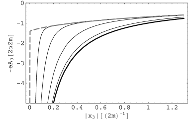
Figure 1: Electron energy $-eA_{0}(x_{3},0)$ in the modified Coulomb potential (41) of the charge $q=Ze$ plotted along the axis $x_{3}$ passing through the charge $q$ parallel to the magnetic field, $x_{\perp}=0$. Thin solid lines correspond to four values of the magnetic field (from left to right): $b=10^{6},\;b=10^{5}$, $b=10^{4}$ and $b=10^{3}$. Bold solid line is the Coulomb law $A_{0}^{\rm C}(x_{3},0)=q/(4\pi x_{3})$. Thin lines approach asymptotically the bold line at the both edges of the figure. Thick dashed broken line corresponds to $b=\infty$. The abscissa represents the distance in the units $(2m)^{-1}$. The ordinate represents the potential in the units $2Z\alpha m=Z\times 7.46$ keV.

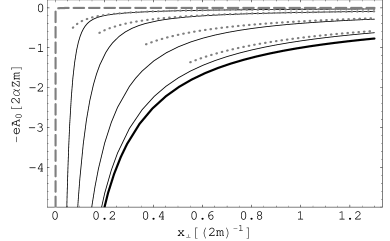
Figure 2: Electron energy $-eA_{0}(0,x_{\perp})$ in the modified Coulomb potential (41) plotted along the axis $x_{\perp}$ passing through the charge $q$ transversely to the magnetic field, $x_{3}=0$. Conventions are the same as in Fig. 1. Thin lines approach asymptotically the solid line at the left lower edge of the figure and the short dotted lines (IV.1.1) $A_{0}(0,x_{\perp})=q/(4\pi x_{\perp}^{\prime})$ at the upper right edge.

The nontrivial - other than the leading asymptote $\sim k_{3}^{2}$ near the point $k_{3}=k_{\perp}=0$ - dependence of the polarization operator eigenvalue (38) on the photon momentum components $k_{3}$, $k_{\perp}$ is the spatial dispersion. We shall see in Section 3 that it is important in the vicinity of the charge, where the field has a large gradient. As for the anisotropic behavior far from the charge, to be studied in Section 4, only the above asymptote is essential, inferable also from the Heisenberg-Euler Lagrangian.

In Appendix 1 we consider the singular asymptotic behavior of the potential in the vicinity of the point charge and present its expansion near $|{\bf x}|=0$. Now we shall consider separately two additive parts of the potential that decrease by different ways with increase of the distance ${\bf x}$.

It is useful to subdivide identically the potential (41) as:

$$A_{0}({\bf x})=A_{\rm s.r.}({\bf x})+A_{\rm l.r.}({\bf x})$$ (42)

with

$$A_{\rm s.r.}({\bf x})=\frac{q}{2(2\pi)^{2}}\int_{0}^{\infty}J_{0}(k_{\perp}x_{\perp})\left[\int_{-\infty}^{\infty}\frac{{\rm e}^{-{\rm i}k_{3}x_{3}}{\rm d}k_{3}}{k_{\perp}^{2}+k_{3}^{2}+{2\alpha bm^{2}\over\pi}\exp\left(-{k_{\perp}^{2}\over 2m^{2}b}\right)}\right]{\rm d}k_{\perp}^{2}$$ (43)

and

$$A_{\rm l.r.}({\bf x})=\frac{q}{2(2\pi)^{2}}\int_{0}^{\infty}J_{0}(k_{\perp}x_{\perp})\int_{-\infty}^{\infty}{\rm e}^{-{\rm i}k_{3}x_{3}}{\rm d}k_{3}\hskip 142.26378pt$$

$$\times\left[\frac{1}{k_{\perp}^{2}+k_{3}^{2}+\frac{2\alpha bm^{2}}{\pi}\exp\left(-\frac{k_{\bot}^{2}}{2m^{2}b}\right)T\left({k_{3}^{2}\over 4m^{2}}\right)}-\frac{1}{k_{\perp}^{2}+k_{3}^{2}+\frac{2\alpha bm^{2}}{\pi}\exp\left(-\frac{k_{\bot}^{2}}{2m^{2}b}\right)}\right]{\rm d}k_{\perp}^{2}.$$ (44)

Eq. (43) is the potential (34) or (41) taken with the substitution $T\left({k_{3}^{2}\over 4m^{2}}\right)\Rightarrow T(\infty)=1$ inside $\kappa_{2}$ (38). We shall see in what follows that $A_{\rm s.r.}({\bf x})$ is a Yukawa-like potential, singular in the origin, that exponentially decreases at distances of about $\sqrt{\pi/2\alpha}\simeq 15L_{\rm B}$, while $A_{\rm l.r.}({\bf x})$ is a finite function that slowly decreases at large distances (greater than the Compton length $m^{-1}$) following what will be called anisotropic Coulomb law. This is the reason why we shall call Eq. (43) the short-range part and Eq. (II) the long-range part of the potential.

Consider first the short-range part (43) and the limiting form it takes in the infinite-field limit.

III Short-range part

III.1 The scaling regime

It is remarkable to note that the short-range part of the potential (43), as measured in the inverse Larmour length $L_{\rm B}^{-1}=\sqrt{eB}$ units is a universal, magnetic-field-independent function of coordinates measured in Larmour units $L_{\rm B}$. To establish this scaling regime let us make the change of variables in the integral (43) $\widetilde{k}_{3}=k_{3}L_{\rm B},$ $\widetilde{k}_{\perp}=k_{\perp}L_{\rm B}$ and define the new dimensionless coordinates $x_{3}=\widetilde{x}_{3}L_{\rm B},$ $x_{\perp}=\widetilde{x}_{\perp}L_{\rm B}.$ Then Eq. (43) becomes

$$A_{\rm s.r.}({\bf x})=\frac{q}{2(2\pi)^{2}L_{\rm B}}\int_{0}^{\infty}J_{0}(\widetilde{k}_{\perp}\widetilde{x}_{\perp})\int_{-\infty}^{\infty}\frac{{\rm e}^{-{\rm i}\widetilde{k}_{3}\widetilde{x}_{3}}{\rm d}\widetilde{k}_{3}{\rm d}\widetilde{k}_{\perp}^{2}}{\widetilde{k}_{\perp}^{2}+\widetilde{k}_{3}^{2}+\frac{2\alpha}{\pi}\exp\left(-\frac{\widetilde{k}^{2}_{\perp}}{2}\right)}.$$ (45)

This is an even function of $x_{3}$. The $\widetilde{k}_{3}$-integration here can be performed by calculating the residues in the poles on the imaginary axis in the points

$$\widetilde{k}_{3}=\pm{\rm i}\sqrt{\widetilde{k}_{\perp}^{2}+\frac{2\alpha}{\pi}\exp\left(-\frac{\widetilde{k}^{2}_{\perp}}{2}\right)}$$ (46)

with the upper sign taken for $x_{3}>0$ and the lower one for $x_{3}<0$. Finally one gets

$$A_{\rm s.r}({\bf x})=\frac{\widetilde{A}(\widetilde{\bf x})}{L_{\rm B}}=\frac{q}{8\pi L_{\rm B}}\int_{0}^{\infty}J_{0}(\widetilde{k}_{\perp}\widetilde{x}_{\perp})\frac{{\rm e}^{-|\widetilde{x}_{3}|\sqrt{\widetilde{k}_{\perp}^{2}+\frac{2\alpha}{\pi}\exp\left(-\frac{\widetilde{k}_{\perp}^{2}}{2}\right)}}}{\sqrt{\widetilde{k}_{\perp}^{2}+\frac{2\alpha}{\pi}\exp\left(-\frac{\widetilde{k}^{2}_{\perp}}{2}\right)}}{\rm d}\widetilde{k}^{2}_{\perp}.$$ (47)

Here the universal function $\widetilde{A}(\widetilde{\bf x})$ depends on the magnetic field through its spatial arguments $\widetilde{\bf x}$ only. Eq. (43) (or (45) and (47)) is illustrated in Fig. 3 drawn for $x_{\perp}=0$ by a computer.

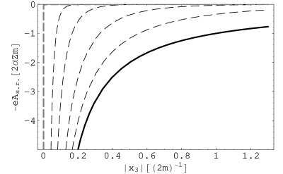
Figure 3: Electron energy $-eA_{\rm s.r.}(x_{3},0)$ in the short-range part Eq. (43) of the potential plotted against the (absolute value of) longitudinal distance $x_{3}$ for $x_{\perp}=0$ (thin dashed lines from left to right correspond to $b=10^{6},\;10^{5},\;10^{4},\;10^{3}$). The thick dashed broken line corresponds to $b=\infty$. All the rest is the same as in Figs 1 and 2.

The simple representation (47) can be further simplified if $x_{3}$ or $x_{\perp}$ are large in the Larmour scale: $|\widetilde{x}_{3}|\gg 1,$ or $|\widetilde{x}_{\perp}|\gg 1.$ In this case the integration in (47) is restricted to the domain $\widetilde{k}_{\perp}^{2}\ll 1$ where the exponential $\exp(-\widetilde{k}_{\perp}^{2}/2)$ should be taken as unity. Then (47) is reduced to the Yukawa law for the short-range part of the potential

$$A_{\rm s.r.}({\bf x})\simeq A_{0}^{\rm Y}({\bf x})=\frac{q}{4\pi L_{\rm B}}\frac{\exp\,[-(2\alpha/\pi)^{1/2}{\sqrt{\widetilde{x}_{\perp}^{2}+\widetilde{x}_{3}^{2}}}\,]}{\sqrt{\widetilde{x}_{\perp}^{2}+\widetilde{x}_{3}^{2}}}=\frac{q}{4\pi}\frac{\exp\,[-(2\alpha b/\pi)^{1/2}m|{\bf x}|\,]}{|{\bf x}|}.$$ (48)

It reflects the Debye screening of the charge by the polarized vacuum. Eq. (48) can be established if we return to the previous representation (45), which can then be traced back to (41) with

$$-\kappa_{2}(0,\infty,0)=\frac{2\alpha}{\pi L_{\rm B}^{2}}T(\infty)=m^{2}\frac{2\alpha b}{\pi}\equiv M^{2}$$ (49)

substituted for $-\kappa_{2}(0,k_{3}^{2},k_{\perp}^{2})$ in the denominator. Here $M$ is the ”effective photon mass”  of Ref. kuznets . Write it as

$$M=\frac{e}{\pi\sqrt{2}\;L_{\rm B}}.$$ (50)

The deviation of (47) from (48) when $\widetilde{x}_{\perp}$ and $\widetilde{x}_{3}$ are both small is not very important against the background of the singularity of the short-range part of the potential $A_{\rm s.r.}({\bf x})$ near the charge provided by the divergency of (43) in the origin $\bf x$=0. (See Appendix 1 for the asymptotic expansion of the potential near the origin). Therefore, the Yukawa law (48) is approximately fulfilled also in the close vicinity of the charge. Correspondingly, the curves in Fig. 3 could not be distinguished from the Yukawa law (48) in the scale of the figure.

Eqs. (47) and (48) establish the short-range character of the static electromagnetic forces in the Larmour scale. The corresponding effective mass (49) coincides with the topological photon mass $e_{\rm Sch}/\sqrt{\pi}$ in the 2-dimensional Schwinger electrodynamics schwinger provided that the dimensional fermion charge $e_{\rm Sch}$ of that theory is identified as $e_{\rm Sch}=\sqrt{\pi/2}\;e/L_{\rm B}$. Stress that the zero photon mass understood as its rest energy is also present as a consequence of the gauge invariance reflected in the approximation-independent relation $\kappa_{a}(0,0,0)=0.$ Correspondingly, the potential, produced by a static charge, should be long-range for sufficiently large distances. This is the case, indeed. The long-range character of the electromagnetic interaction is restored at the distances of the Compton scale, as we shall see in the next Section. The carrier of the long-ranged interaction will be $A_{\rm l.r.}({\bf x})$ (II). The Debye screening obtained here in the vacuum completely depends on the fact that the function (39) tends to unity for large longitudinal momentum $k_{3}\to\infty$, i.e. on spatial dispersion. In this point the situation is different from the case of a medium, where the Debye screening can be achieved zeitlin in expressions, obtained from the thermodynamical potential, which is the analog of the effective Lagrangian for that case. The difference with the medium is also in that the long-range part of the $static$ potential is absent in that case in spite of the gauge invariance, because it implies that the appropriate polarization tensor components should disappear in the long-wave limit $k_{0}=0$, $\bf k$=0 only if $\bf k$ is set equal to zero first fradkin , thus providing the zero value to the photon $magnetic$ mass.

III.2 The limiting $b=\infty$ form

The short-range part (43) and (45) tends to zero, when $b\rightarrow\infty$ for any nonzero distance, ${\bf x}\neq 0$, from the charge. This follows from the fact that $\widetilde{A}(\widetilde{x})$, defined in (47), tends to zero with the exponential speed (48) when $\widetilde{x}_{3}=x_{3}/L_{\rm B}$ or $\widetilde{x}_{\perp}=x_{\perp}/L_{\rm B}$ tends to infinity. As the magnetic field $b$ grows more and more, the curves representing the potential (47) for the special case of $x_{\perp}=0$ in Fig. 3 stick closer and closer to the vertical axis, the spacing between the curves and this axis becoming infinitely thin in the limit $b=\infty$. The area $(q/2\pi)S$ of the region restricted by any curve (47) and the $x_{3}$-axis in the domain $-\infty<x_{3}\leq-L_{\rm B},\;L_{\rm B}\leq x_{3}<\infty$

$$\frac{q}{2\pi}S=2\int^{\infty}_{L_{\rm B}}A_{\rm s.r.}(x_{3},0){\rm d}x_{3}=2\int^{\infty}_{1}\widetilde{A}(\widetilde{x}_{3},0){\rm d}\widetilde{x}_{3}=\frac{q}{4\pi}\int_{0}^{\infty}\frac{{\rm e}^{-\sqrt{\widetilde{k}_{\perp}^{2}+\frac{2\alpha}{\pi}\exp\left(-\frac{\widetilde{k}_{\perp}^{2}}{2}\right)}}{\rm d}\widetilde{k}^{2}_{\perp}}{\widetilde{k}_{\perp}^{2}+\frac{2\alpha}{\pi}\exp\left(-\frac{\widetilde{k}_{\perp}^{2}}{2}\right)}$$ (51)

is a finite number, with $S=2.180$, independent of the magnetic field. If the Yukawa approximation (48) is used in (51) in place of (47), approximately the same numerical value for $S$ is achieved: $S=-{\rm Ei}(-\sqrt{2\alpha/\pi})\simeq 2.176$, where

$${\rm Ei}(u)=-\int_{-u}^{\infty}\exp(-y)y^{-1}{\rm d}y$$ (52)

is the exponential integral. In the limit $b=\infty$, $L_{\rm B}=0$ the width of the strip $|x_{3}|\leq L_{\rm B}$ excluded from the integration in Eq. (51) is zero, and the latter becomes the whole area above the limiting potential. Thus, in the infinite-magnetic-field limit the short-range part (43) of the potential taken on the axis drawn through the point charge $q$ along the magnetic field direction becomes the $\delta$-function:

$$\left.A_{\rm s.r.}(x_{3},0)\right|_{b=\infty}=2.180\frac{q}{2\pi}\delta(x_{3}).$$ (53)

The limiting $\delta$-function here is understood in the following sense. Given a test-function $t(x_{3})$, one has

$$\lim_{b\rightarrow\infty}\left[\int^{-L_{\rm B}}_{-\infty}A_{\rm s.r.}(x_{3},0)t(x_{3}){\rm d}x_{3}+\int_{L_{\rm B}}^{\infty}A_{\rm s.r.}(x_{3},0)t(x_{3}){\rm d}x_{3}\right]=2.180\frac{q}{2\pi}t(0).$$ (54)

[This equation directly follows from the scaling law, the first equality in (47)]. In this sense it will be used in Section IV and Appendix 2, where we shall see that the $\delta$-singularity of the potential (53) leads only to a finite contribution to the atomic ground-state energy in an infinite magnetic field in contrast to the contribution of the primary Coulomb potential.

Analogously, we may write a $\delta$-function for the limiting form of the short-range part of the potential along any direction $x$, $|x|=x_{\perp}$, in the plane orthogonal to the magnetic field containing the point charge $q$. In place of (51) one has

$$\frac{q}{2\pi}S_{\perp}=2\int^{\infty}_{L_{\rm B}}A_{\rm s.r.}(0,x){\rm d}x=2\int^{\infty}_{1}\widetilde{A}(0,\widetilde{x}){\rm d}\widetilde{x}=$$

$$=\frac{q}{2\pi}\int_{0}^{\infty}\frac{1-\widetilde{k}_{\perp}J_{0}(\widetilde{k}_{\perp})+\frac{\pi\widetilde{k}_{\perp}}{2}[J_{0}(\widetilde{k}_{\perp}){\bf H_{1}}(\widetilde{k}_{\perp})-J_{1}(\widetilde{k}_{\perp}){\bf H_{0}}(\widetilde{k}_{\perp})]}{\sqrt{\widetilde{k}_{\perp}^{2}+\frac{2\alpha}{\pi}\exp\left(-\frac{\widetilde{k}_{\perp}^{2}}{2}\right)}}{\rm d}\widetilde{k}_{\perp}=\frac{q}{2\pi}2.178.\quad$$ (55)

Here $J_{0,1}$ and ${\bf H_{0,1}}$ are, resp., the Bessel and Struve functions of orders zero and one. We used the integral 6.512.8 and the representation 8.551.1 in the reference book ryzhik for calculating (III.2). Note that the Struve functions at large argument decrease and oscillate asymptotically like the Neuman functions; besides ${\bf H}_{1}$ includes a constant asymptotic term $2/\pi$. The integral (III.2) converges: the divergence caused by the unity term in the nominator is cancelled by the two products of two oscillating asymptotic terms in the square brackets.

From (III.2) and the fact that for $x_{\perp}\neq 0$ the short-range potential (47) disappears in the $b\to\infty$ limit we have

$$\left.A_{\rm s.r.}(0,x)\right|_{b=\infty}=2.178\frac{q}{2\pi}\delta(x).$$ (56)

The different coefficients in (53) and (56) manifest the anisotropy. Note that the Coulomb singularity of the (short-range part of) the potential in the origin $q/4\pi|{\bf x}|$ is isotropic to avoid .

IV Long-range part

We have finished the consideration of the short-range part and will proceed with considering the long-range part $A_{\rm l.r.}({\bf x})$ (II). Simplifying expressions will be obtained for large-distance behavior in Subsection A and for the long-range part taken on the axis $x_{\perp}=0$ in Subsection B. We shall see in Subsection B that in the limit $b=\infty$ the long-range part, as well as the whole potential, is concentrated on this axis, making an infinitely thin tube or string. We shall study the potential along the string in more detail in Subsection B.

IV.1 Long-distance behavior of the long-range part $A_{\rm l.r.}({\bf x})$

Once we have seen in the previous Section that the short-range part $A_{\rm s.r.}({\bf x})$ is as a matter of fact concentrated within the region of a few $L_{\rm B}$, for larger distances, $|{\bf x}|\gtrsim m^{-1},$ the whole potential (41) and its long-range part (II) are the same. For this reason in this Subsection we shall deal directly with (41).

IV.1.1 Large $x_{\perp}$ in Larmour scale

For large transverse distances the term linearly growing with the magnetic field (38) leads to suppression of the static potential in the transverse direction.

To be more precise, consider the region

$$x_{\perp}\gg\frac{m^{-1}}{\sqrt{2b}}=\frac{L_{\rm B}}{\sqrt{2}}.$$ (57)

Once the Bessel function $J_{0}$ in (41) oscillates and decreases for large values of its argument $k_{\perp}x_{\perp}$, the main contribution into the integral over $k_{\perp}^{2}$ in (41) comes from the integration variable domain $k_{\perp}^{2}\ll 2m^{2}b$, and the dependence upon $k_{\perp}^{2}$ in $\kappa_{2}$ may thus be disregarded. Then the $k_{\perp}^{2}$-integration in (41) can be explicitly performed to give (we use Eq.6.532.4 of the reference book ryzhik )

$$A_{0}(x_{3},x_{\perp})\simeq\frac{2q}{(2\pi)^{2}}\int_{0}^{\infty}\mathcal{K}_{0}\left(x_{\perp}\sqrt{k_{3}^{2}-\kappa_{2}(0,k_{3}^{2},0)}\right)\cos(k_{3}x_{3}){\rm d}k_{3},$$ (58)

where $\mathcal{K}_{0}$ is the McDonald function of order zero, and

$$\kappa_{2}(0,k_{3}^{2},0)=-\frac{2\alpha b}{\pi}m^{2}T\left(\frac{k_{3}^{2}}{4m^{2}}\right).$$ (59)

As the McDonald function $\mathcal{K}_{0}$ decreases exponentially when its argument increases, only small values of the square root contribute into integral (58), and the $k_{3}$-integration domain in it is restricted to the interval $k_{3}^{2}\ll 4m^{2}$, wherein

$$T\left(\frac{k_{3}^{2}}{4m^{2}}\right)\simeq\frac{k_{3}^{2}}{6m^{2}}.$$ (60)

Then the potential form (58) becomes (we use Eq. 6.671.14 of the reference book ryzhik )

$$A_{0}(x_{3},x_{\perp})\simeq\frac{2q}{(2\pi)^{2}}\int_{0}^{\infty}\mathcal{K}_{0}\left(x_{\perp}k_{3}\sqrt{1+\frac{\alpha b}{3\pi}}\right)\cos(k_{3}x_{3}){\rm d}k_{3}$$

$$=\frac{1}{4\pi}\frac{q}{\sqrt{(x^{\prime}_{\perp})^{2}+x_{3}^{2}}},\quad\qquad x^{\prime}_{\perp}=x_{\perp}\left(1+\frac{\alpha b}{3\pi}\right)^{1/2},~{}~{}x^{\prime}_{\perp}>x_{\perp}.$$ (61)

Eq. (IV.1.1) is an anisotropic Coulomb law, according to which the attraction force decreases with distance from the source along the transverse direction faster than along the magnetic field (remind that $b\equiv(B/B_{0})\gg 1$), but remains long-range. The equipotential surface is an ellipsoid stretched along the magnetic field. The electric field of the charge ${\bf E}=-{\bf\nabla}A_{0}(x_{3},x_{\perp}),$ as written in Cartesian components, is the vector $(q/2\pi)(x_{3}^{2}+\beta^{2}x_{\perp}^{2})^{-3/2}~{}(\beta^{2}x_{1}~{}~{}\beta^{2}x_{2}~{}~{}x_{3})$, where $\beta=(1+\alpha b/3\pi)^{1/2}$. It is not directed towards the charge, but makes an angle $\phi$ with the radius-vector $\bf r$, cos$\phi=(x_{3}^{2}+\beta^{2}x_{\perp}^{2})(x_{3}^{2}+\beta^{4}x_{\perp}^{2})^{-1/2}(x_{3}^{2}+x_{\perp}^{2})^{-1/2}.$ If $x_{\perp}\neq 0$, in the limit of infinite magnetic field, $\beta\to\infty$, the electric field of the point charge is directed normally to the axis $x_{3}$, since the ratio $(E_{3}/E_{\perp})\to 0$ (although $E_{3}$ and $E_{\perp}$ are both equal to zero in this limit outside the string). But if $x_{\perp}=0$, the electric field is directed along the external magnetic field. It looks like the electric field compresses the string. This regime corresponds to the dielectric permeability of the vacuum independent of the frequency, with its dependence on $\bf k$ (spatial dispersion) being reduced solely to that upon the angle in the space ($cf,$ zhetf ).

The result (IV.1.1) is in agreement with the curves in Fig. 2 in the large $x_{\perp}$ domain.

IV.1.2 Large $x_{3}$

It remains to consider the remote coordinate region of large $x_{3}$, complementary to (57).

To this end we apply the residue method to the inner integral over $k_{3}$ in (41). Using the integral representation (39) the function $\kappa_{2}$ (38) may be, for a fixed positive value of $k_{\perp}^{2}$, analytically continued from the real values of the variable $k_{3}$ into the whole complex plane of it, cut along two fragments of the imaginary axis. In the lower half-plane the cut runs from Im$~{}k_{3}=-2m$ down to Im $k_{3}=-\infty$, while in the upper half-plane it extends within the limits $2m\leq{\rm Im}~{}k_{3}\leq\infty$. Other singularities of the $k_{3}$-integrand in (41) are poles yielded by zeros of the denominator, i.e. solutions of the equation (associated with the photon dispersion equation)

$$k_{\perp}^{2}+k_{3}^{2}-\kappa_{2}(0,k_{3}^{2},k_{\perp}^{2})=0.$$ (62)

As $k_{\perp}$ varies within the limits $(0,\infty)$ two roots of this equation $k^{\pm}_{3}=\pm{\rm i}K(k_{\perp})$ move along the imaginary axis from the point $K(0)=0$ to the points $k^{\pm}_{3}=\pm{\rm i}K(\infty)=\pm{\rm i}2m$ annphys ; nuovcimlet ; zhetf . There is yet another branch of the solution to equation (62), corresponding to the photon absorption via the $\gamma\rightarrow e^{+}e^{-}$-decay, but the corresponding poles lie in the nonphysical sheet of the described complex plane, behind the cuts, and will not be of importance for the consideration below.

Let us consider positive values of $x_{3}$. Negative values can be handled in an analogous way. Turning the positive part of integration path $0\leq k_{3}\leq\infty$ clockwise to the lower half-plane by the angle $\pi/2$, and the negative part $-\infty\leq k_{3}\leq 0$ counterclockwise by the same angle, and referring to the fact that the exponential $\exp(-{\rm i}k_{3}x_{3})$ decreases, for $x_{3}>0$, in the lower half-plane of $k_{3}$ as $|k_{3}|\rightarrow\infty$ so that the integrals over the remote arcs may be omitted, we get a representation for the inner integral in (41)

$$\int_{-\infty}^{\infty}\frac{{\rm e}^{-{\rm i}k_{3}x_{3}}{\rm d}k_{3}}{k_{\perp}^{2}+k_{3}^{2}-\kappa_{2}(0,k_{3}^{2},k_{\perp}^{2})}$$

$$={\rm i}\int_{2m}^{\infty}{\rm e}^{-|k_{3}|x_{3}}\Delta(|k_{3}|^{2},k_{\perp}^{2})\,{\rm d}|k_{3}|-{\rm i}\,2\pi\exp\,[-K(k_{\perp}^{2})x_{3}\,]\,{\rm Res}(k_{\perp}^{2})\,,$$ (63)

where Res$(k_{\perp}^{2})$ designates the residue of the expression $D_{2}(0,-|k_{3}|^{2},k_{\perp}^{2})=\left(k_{\perp}^{2}-|k_{3}|^{2}-\kappa_{2}(0,-|k_{3}^{2}|,k_{\perp}^{2})\right)^{-1}$ in the pole $k_{3}^{-}=-iK(k^{2}_{\perp})$, while $\Delta(|k_{3}|^{2},k_{\perp}^{2})=D_{2}(0,-|k_{3}|^{2}+{\rm i}0,k_{\perp}^{2})-D_{2}(0,-|k_{3}|^{2}-{\rm i}0,k_{\perp}^{2})$ is the cut discontinuity. It was explained above that $0<K(k_{\perp}^{2})<2m$ everywhere but in the limit $k_{\perp}\rightarrow\infty$, where $K=2m$. Consequently the residue term in (IV.1.2) dominates over the cut-discontinuity term everywhere in the $k_{\perp}$-integration domain in the outer integral in (41), except for the region near $k_{\perp}=\infty$. In this limit, however, $\kappa_{2}$ disappears due to the exponential in (38), together with the cut discontinuity, since the latter is only due to the branching points in the function (39). Therefore, keeping the residue term in (IV.1.2) as the leading one, we neglect the contribution that decreases with large longitudinal distance at least as fast as $\exp(-2m|x_{3}|).$ In this way we come to the asymptotic representation of the potential (41) in the region of large longitudinal distances $|x_{3}|\gg(2m)^{-1}$ (negative values of $x_{3}$ at this step are also included - to handle them one should rotate the fragments of the integration path in the directions opposite to the above)

$$A_{0}({\bf x})\simeq\frac{q}{8\pi}\int_{0}^{\infty}\frac{J_{0}(k_{\perp}x_{\perp})\,\exp\,[-K(k^{2}_{\perp})|x_{3}|]\,{\rm d}k^{2}_{\perp}}{K(k^{2}_{\perp})[1+H(-K^{2}(k^{2}_{\perp}),k_{\perp}^{2})]},$$ (64)

where

$$H(k_{3}^{2},k_{\perp}^{2})=\frac{2\alpha bm^{2}}{\pi}\exp\left(-\frac{k_{\perp}^{2}}{2m^{2}b}\right)\frac{{\rm d}}{{\rm d}k_{3}^{2}}T\left(\frac{k_{3}^{2}}{4m^{2}}\right).$$ (65)

Here $K^{2}(k_{\perp}^{2})$ is the solution of equation (62) in the negative region of the variable $k_{3}^{2}$ - see zhetf for its form. $K(\infty)=2m$, $K(0)=0$. $T$ is given by (39).

Due to the exponential factor in the integrand of (64), for large $x_{3}$ the main contribution comes from the integration region of $k_{\perp}$ that provides minimum to the function $K(k_{\perp})$. The minimum value of $K(k_{\perp})$ is zero. It is achieved in the point $k_{\perp}=0$ - a manifestation of the fact that the photon mass defined as its rest energy is strictly equal to zero owing to the gauge invariance: $\kappa_{a}(k_{0}=k_{3}={\bf k}=0)=0$. In view of (59) and (60), near the point $k_{\perp}=0$ the dispersion equation (62) has the solution $K(k_{\perp})=k_{\perp}/\sqrt{1+\alpha b/3\pi}$. Simultaneously, near the minimum point $1+H(0,0)=1+\alpha b/3\pi$. With these substitutions and the use of 6.611.1 of ryzhik , Eq. (64) becomes again the anisotropic Coulomb law (IV.1.1) $(q/4\pi)/[(x^{\prime}_{\perp})^{2}+x_{3}^{2}]^{1/2}$. We have, therefore, established its validity everywhere in the region remote from the center, irrespectively of the direction.

In agreement with this result the curves in Fig. 1 for $A_{0}(x_{3},0)$ approach the Coulomb law $q/4\pi|x_{3}|$ as $|x_{3}|$ grows.

Figure 4: Electron energy $-eA_{0}(x_{3},x_{\perp})$ in the modified Coulomb potential (64) with $q=Ze$ plotted against the transverse coordinate $x_{\perp}$ with the longitudinal coordinate fixed at the large value $x_{3}=10(2m)^{-1}$. Thin solid line corresponds to the magnetic field value $B=10^{4}B_{0}$. Bold solid line is the standard Coulomb law (5) $-eA_{0}^{\rm C}(x_{3},x_{\perp})=-2\alpha Zm[(2mx_{\perp})^{2}+100]^{-1/2}$. The thin line is indistinguishable from the anisotropic Coulomb law (IV.1.1) in the scale of the drawing. The coordinate axes are the same as in Fig. 2

The difference between the potential $A_{0}(x_{3},0)$ and its large-$x_{3}$ asymptote $q/4\pi|x_{3}|$ decreases in Fig. 1 at least as fast as exp$(-2m|x_{3}|)$ (see arxive for the derivation of the latter statement).

Eq. (64) was used for computer calculation with the large value $x_{3}=10m^{-1}$. It has led to the curve shown in Fig. 4. In the region (57) it agrees with the result (IV.1.1), valid in that region [$L_{\rm B}=0.02(2m)^{-1}$ for $b=10^{4}$]. In practice (64) and (IV.1.1) are the same. A small deviation of the potential curve $A_{0}(10/2m,x_{\perp})$ from (IV.1.1) may be seen in Fig. 5 of Ref. arxive , drawn in a more detailed scale for small $x_{\perp}$.

IV.2 The long-range part on the axis $x_{\perp}=0$ and its limiting form for $b=\infty$

Curves drawn for $A_{\rm l.r.}(x_{3},0)$ by a computer following Eq. (II) are presented in Fig. 5.

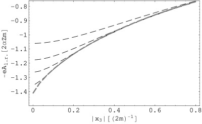
Figure 5: Electron energy $-eA_{\rm l.r.}(x_{3},0)$ in the long-range part (II) of the potential for $b=\infty$ (dashed thick line) and $b=10^{6},\;10^{5}$, $3\times 10^{4}$, $10^{4}$ (dashed lines from bottom to top)

Here we study the form the long-range part (II) of the potential takes in the limit $b=\infty$.

First consider the case $x_{\perp}\neq 0,\;x_{3}\neq 0$. As we saw in Subsection B of Section 3 the short-range part of the potential tends in this case to zero as $b\rightarrow\infty$. Therefore, the limits of the whole potential and of its long-range part are the same. For this reason to achieve the claimed goal it is sufficient to consider the limit of (41). After the change of the integration variable $k_{\perp}=\widetilde{k}_{\perp}m\sqrt{b}\;$ Eq. (41) becomes

$$A_{0}({\bf x})=\frac{q}{2(2\pi)^{2}}\int_{0}^{\infty}J_{0}(\widetilde{k}_{\perp}m\sqrt{b}x_{\perp})\int_{-\infty}^{\infty}\frac{{\rm e}^{-{\rm i}k_{3}x_{3}}{\rm d}k_{3}{\rm d}\widetilde{k}_{\perp}^{2}}{\widetilde{k}_{\perp}^{2}+{k_{3}^{2}\over m^{2}b}+\frac{2\alpha}{\pi}\exp\left(-\frac{\widetilde{k}_{\bot}^{2}}{2}\right)T\left({k_{3}^{2}\over 4m^{2}}\right)}$$ (66)

When $b\gg(\pi/2\alpha)$ one can disregard the ratio ${k_{3}^{2}\over m^{2}b}$ in the denominator.

For any finite $x_{\perp}$ the argument of the Bessel function in (66) is large, therefore we may use the same procedure as the one that led us from (41) to (58) and (IV.1.1). Then we obtain

$$\left.A_{0}(x_{3},x_{\perp})\right|_{b\rightarrow\infty,\;x_{\perp}\neq 0}=\frac{2q}{(2\pi)^{2}}\int_{0}^{\infty}\mathcal{K}_{0}\left(x_{\perp}k_{3}\sqrt{\frac{\alpha b}{3\pi}}\right)\cos(k_{3}x_{3}){\rm d}k_{3}$$

$$={1\over 4\pi}\frac{q}{\sqrt{x_{\perp}^{2}(\alpha b/3\pi)+x_{3}^{2}}}\simeq{qm\over 4\sqrt{\alpha\pi/3}}{L_{\rm B}\over x_{\perp}}\rightarrow 0.$$ (67)

This means that outside the $x_{3}$-axis the potential (41) turns to zero as the ratio $L_{\rm B}/x_{\perp}$. Since its short-range part (43) or (48) decreases with $b$ exponentially, the result (IV.2) holds for the long-range part (II) as well.

The situation is different on the axis $x_{\perp}=0$. By making in Eq. (II) the same change of the variable $k_{\perp}$ as above and, again, neglecting $k_{3}^{2}/4m^{2}b$ in the denominators we come to the limiting ($b=\infty$) form of the long-range part of the potential $x_{\perp}=0$, independent of the magnetic field

$$\left.A_{\rm l.r.}(x_{3},0)\right|_{b=\infty}=\frac{q}{(2\pi)^{2}}\int_{0}^{\infty}\int_{0}^{\infty}\cos(k_{3}x_{3}){\rm d}k_{3}\hskip 142.26378pt$$

$$\times\left\{\frac{1}{\widetilde{k}_{\perp}^{2}+\frac{2\alpha}{\pi}\exp\left(-\frac{\widetilde{k}_{\perp}^{2}}{2}\right)T\left({k_{3}^{2}\over 4m^{2}}\right)}-\frac{1}{\widetilde{k}_{\perp}^{2}+\frac{2\alpha}{\pi}\exp\left(-\frac{\widetilde{k}_{\perp}^{2}}{2}\right)}\right\}{\rm d}\widetilde{k}_{\perp}^{2}.$$ (68)

This is the analytic representation of the envelope curve in Fig. 1. To understand this, note that the overall potential is the sum of the short- and long-range parts, according to (42). Therefore by combining the curves in Figs. 3 and 5 we come to the pattern presented in Fig. 6, which is the detailing of Fig. 1. Each potential curve drawn for a certain value of the magnetic field approaches, as the distance from the charge along the $x_{3}$-axis grows, the corresponding (dashed) curve transferred from Fig. 5. But even prior to this, the latter approaches the thick dashed curve, which is the common envelope of the curves in Fig. 5 and the whole potential curves in Figs. 1 and 6.

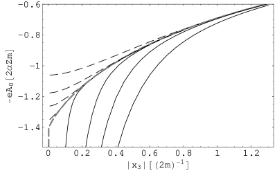
Figure 6: Four electron energy $-eA_{0}(x_{3},0)$ curves in the modified potential (41) for $b=10^{6},\,10^{5},\,3\times 10^{4},\,{\rm and}\,10^{4}$ (thin solid lines from left to right) approaching their corresponding long-range parts $-eA_{\rm l.r.}(x_{3},0)$, Eq. (II), shown in Fig. 5 (four dashed lines from bottom to top). Thick dashed broken line corresponds to the string potential $A_{0}(x_{3},0)\left.\right|_{b=\infty}$. Its vertical fragment symbolizes the $\delta$-function (54).

We continue by studying the long-range part of the potential along the string, Eq. (IV.2). To separate the part independent of the fine-structure constant $\alpha$ the internal integral here is integrated by parts to yield:

$$\int_{0}^{\infty}\left({{\rm d}\over{\rm d}\widetilde{k}_{\perp}^{2}}\ln\frac{\widetilde{k}_{\perp}^{2}+{2\alpha\over\pi}\exp\left({-\widetilde{k}_{\perp}^{2}\over 2}\right)T(y)}{\widetilde{k}_{\perp}^{2}+{2\alpha\over\pi}\exp\left({-\widetilde{k}_{\perp}^{2}\over 2}\right)}\right)\frac{\;{\rm d}\widetilde{k}_{\perp}^{2}}{1+{\widetilde{k}_{\perp}^{2}\over 2}}\hskip 128.0374pt$$

$$=-\ln T\left(y\right)+{1\over 2}\int_{0}^{\infty}\frac{{\rm d}\widetilde{k}_{\perp}^{2}}{\left(1+{\widetilde{k}_{\perp}^{2}\over 2}\right)^{2}}\ln\frac{\widetilde{k}_{\perp}^{2}+{2\alpha\over\pi}\exp\left({-\widetilde{k}_{\perp}^{2}\over 2}\right)T(y)}{\widetilde{k}_{\perp}^{2}+{2\alpha\over\pi}\exp\left({-\widetilde{k}_{\perp}^{2}\over 2}\right)}.$$ (69)

Then (IV.2) becomes

$$\left.A_{\rm l.r.}(x_{3},0)\right|_{b=\infty}=\left.A_{\rm l.r.}(x_{3},0)\right|_{b=\infty,\alpha=0}\hskip 199.16928pt$$

$$+\frac{q}{2(2\pi)^{2}}\int_{0}^{\infty}\int_{0}^{\infty}\frac{\cos(k_{3}x_{3}){\rm d}k_{3}{\rm d}\widetilde{k}_{\perp}^{2}}{\left(1+{\widetilde{k}_{\perp}^{2}\over 2}\right)^{2}}\ln\left\{1+\frac{{2\alpha\over\pi}\exp\left({-\widetilde{k}_{\perp}^{2}\over 2}\right)\left[T\left({k_{3}^{2}\over 4m^{2}}\right)-1\right]}{\widetilde{k}_{\perp}^{2}+{2\alpha\over\pi}\exp\left({-\widetilde{k}_{\perp}^{2}\over 2}\right)}\right\},\hskip 28.45274pt$$ (70)

where the first term (it is worth recalling here that within the integration limits $T(y)$ is a positive function, lesser than unity)

$$\left.A_{\rm l.r.}(x_{3},0)\right|_{b=\infty,\alpha=0}=-\frac{q}{(2\pi)^{2}}\int_{0}^{\infty}\cos(k_{3}x_{3})\ln\left[T\left({k_{3}^{2}\over 4m^{2}}\right)\right]{\rm d}k_{3}$$ (71)

is independent of $\alpha$, whereas the second term behaves as

$$\frac{q}{4\pi^{3}}(-\alpha\ln\alpha)\int_{0}^{\infty}\cos(k_{3}x_{3})\left[T\left({k_{3}^{2}\over 4m^{2}}\right)-1\right]{\rm d}k_{3}.$$ (72)

when $\alpha$ tends to zero, i.e. is nonanalytic in $\alpha=0$. The reason for the nonanalyticity and for the nonvanishing of $\left.A_{\rm l.r.}(x_{3},0)\right|_{b=\infty,\alpha=0}$ is in that that a chain of diagrams has been as a matter of fact summed when solving the Dyson-Schwinger equation that led to the expression for the photon Green function (II) with the one-loop polarization operator (38) substituted into it. In the result (34) thus obtained the two limits $b=\infty$ and $\alpha=0$ are not permutable.

Eq. (71) may be referred to as a fitting approximation for the envelope (IV.2), simpler than (IV.2). It is presumably useful for making rough estimates with the accuracy to $(-\alpha/\pi)\ln\alpha=0.011$. It might have been obtained if the exponential $\exp(-\widetilde{k}_{\perp}^{2}/2)$ in (IV.2) had been merely replaced by unity. The integral (71) is converging at the both integration limits due to the asymptotic properties of the function $T(y)$ indicated below its definition (39) and represents a function that decreases at large longitudinal distances following the Coulomb law $(q/4\pi x_{3}).$

The limiting curve (IV.2), or (IV.2), (71) for the long-range part of the potential (II) crosses the axis $x_{3}=0$ in the point $\left.A_{\rm l.r.}(0,0)\right|_{b=\infty}=(1.4240-0.0088)(qm/2\pi)=1.4152(qm/2\pi)$. Here two numerical contributions from the first and the second terms in (IV.2) are presented separately. It is intriguing how close the numerical coefficient in the expression for the intercept of the envelope and the $x_{3}=0$ axis is to $\sqrt{2}=1.4142$. More precise value of $\sqrt{2}$ would be achieved by the infinite-magnetic-field limit of the long-range part of the potential in the point where its charge is located, if the fine-structure constant were 1/121. Higher-loop calculations may improve this figure.

Identifying the above-calculated $\alpha$-dependent coefficient 1.4152 supposedly with $\sqrt{2}$, an interesting observation would follow: if the charge $q$ is taken equal to the electron charge $e$, $(Z=1)$, the string potential undergoes the increment between the point $x_{3}$ where the charge is located and the infinitely remote point $x_{3}=\infty$, equal to

$$\Delta A_{\rm l.r.}(x_{3})\equiv A_{\rm l.r.}(0,0)\left.\right|_{b=\infty}-A_{\rm l.r.}(\infty,0)\left.\right|_{b=\infty}=\frac{e}{\pi\sqrt{2}\;\lambda_{\rm C}},$$ (73)

where $\lambda_{\rm C}=m^{-1}$ is the Compton length. This ”work function over a unit charge” differs from the photon mass (50) in that the Larmour dimensioning has been replaced by the Compton one.

In the interval $|x_{3}|\ll(2m)^{-1}$ the envelope curve (IV.2) looks roughly in Fig. 1 as a linearly growing potential, the same as this is believed to be the case for the confining potential along quark-antiquark string in QCD in the limit of zero lattice spacing. We may say that in QED the ”confinement” occurs within distances smaller than the Compton length, whereas for larger distances - thanks to the fact that the infrared behavior in QED is weaker than in QCD - the growth of the potential ceases and it approaches the zero value along the Coulomb asymptote. As a matter of fact the growth of the potential is only nearly linear.

To establish its true character consider the difference $\left.A_{\rm l.r.}(x_{3},0)\right|_{b=\infty}-\left.A_{\rm l.r.}(0,0)\right|_{b=\infty}$ and change to the new integration variable $u=k_{3}x_{3}$ in the integrals (71) and (IV.2). Then the argument of the function $T(y)$ becomes $(u^{2}/4m^{2}x_{3}^{2})$ and should be considered as large, once $4m^{2}x_{3}^{2}\ll 1$. According to Eq. (39) for large $y$ one has $[T(y)-1]\simeq(-\ln 2y/2y)$. As long as this tends to zero with $y\rightarrow\infty$, we may substitute $\ln(1+x)\approx x,\;x\ll 1$ for the logarithms in (71) and (IV.2). In this way we obtain

$$\left.A_{\rm l.r.}(x_{3},0)\right|_{b=\infty}-\left.A_{\rm l.r.}(0,0)\right|_{b=\infty}=\frac{qm}{4\pi}\left(1-{\alpha\over\pi}f(\alpha)\right)2m|x_{3}|\left[\ln(2m|x_{3}|)-{1\over 2}\ln 2+\gamma-1\right],\quad$$ (74)

where

$$f(\alpha)=\int_{0}^{\infty}\frac{\exp\left({-\widetilde{k}_{\perp}^{2}\over 2}\right){\rm d}\widetilde{k}_{\perp}^{2}}{\left(1+{\widetilde{k}_{\perp}^{2}\over 2}\right)^{2}\left[\widetilde{k}_{\perp}^{2}+{2\alpha\over\pi}\exp\left({-\widetilde{k}_{\perp}^{2}\over 2}\right)\right]},\quad f\left({1\over 137.036}\right)=4.533,\quad\left.f(\alpha)\right|_{\alpha\rightarrow 0}\simeq-\ln\alpha,\qquad$$ (75)

and $\gamma=0.577$ is the Euler constant. We have made use of the two standard integrals ryzhik

$$\int_{0}^{\infty}\frac{(\cos u-1)}{u^{2}}~{}{\rm d}u=-{\pi\over 2},\qquad\qquad\int_{0}^{\infty}\frac{(\cos u-1)}{u^{2}}\;\ln u\;{\rm d}u={\pi\over 2}(\gamma-1).$$ (76)

Finally, for small distances along the string, $2|x_{3}|m\ll 1$, the long-range potential has the form:

$$\left.A_{\rm l.r.}(x_{3},0)\right|_{b=\infty}=\frac{qm}{2\pi}[1.4152+0.495\times 2m|x_{3}|(\ln(2m|x_{3}|)-0.77)],$$ (77)

This should be additively combined with the $\delta$-function (53), to which the short-range part $A_{s.r.}(x_{3},0)$ is reduced in the limit $b=\infty$, to form the string potential. It is this potential that is responsible for forming the spectrum of an atom in the strong magnetic field, to consideration of which we are proceeding.

V Radiative shift of electron ground-state energy in a hydrogenlike atom in a strong magnetic field

In this section we shall study how the ground-state energy of a hydrogenlike atom at rest in a strong magnetic field is modified by the radiative corrections to the Coulomb potential considered above.

The nonrelativistic electron in an atom, whose nucleus has the charge $q=Ze$, is described by the one-dimensional Schr$\ddot{\rm o}$dinger equation elliott

$$-\frac{1}{2m}\frac{{\rm d}^{2}\Psi(x_{3})}{{\rm d}x_{3}^{2}}-eA_{0}(x_{3},x_{\perp}=0)\Psi(x_{3})=E\Psi(x_{3}),\qquad|x_{3}|>L_{\rm B}=(eB)^{-1/2},$$ (78)

if the atom does not move transverse to the magnetic field - which is the case as long as we are interested in its ground state. The one-dimensional Schr$\ddot{\rm o}$dinger equation (78) is valid in the region $|x_{3}|>L_{\rm B}$ and is efficient provided that $L_{\rm B}\ll a_{\rm B}/Z$, where $a_{\rm B}=1/m\alpha$ is the Bohr radius.

If the unmodified Coulomb potential (4) taken at $x_{\perp}=0$ is used for $A_{0}(x_{3},0)$ in equation (78) ($q=Ze$ henceforward), the ground-state energy value

$$E_{0}=-2Z^{2}\alpha^{2}m\ln^{2}\frac{\sqrt{b}}{2\alpha Z},$$ (79)

that follows elliott ; haines from equation (78) is unbounded from below, in other words tends to negative infinity as the magnetic field grows. The reason is that the one-dimensional Coulomb potential is too singular, the singularity being regularized by the Larmour radius. In equation (78) this regularization acts as the cut-off of the definition region $|x_{3}|>L_{\rm B}$ of equation (78). The regularization is lifted by letting $b$ tend to infinity, $L_{\rm B}\to 0,$ and hence $E_{0}\to-\infty$. On the contrary, the radiation corrections studied here, yielded the conclusion that the Coulomb $q/(4\pi x_{3})$ singularity of the one-dimensional potential in $x_{3}=0$ had been changed to the $\delta$-function (53). This sort of singularity is not expected to cause an unboundedness of the energy spectrum. To confirm this, we solve in Appendix II the Schr$\ddot{\rm o}$dinger equation (78) with a potential that models the short-range part $A_{\rm s.r.}(x_{3},0)$ (43) alone and also tends to $\delta$-function as $b\to\infty$. The resulting ground-state energy approaches in this limit the finite, magnetic-field-independent value given by Eq. (130) of Appendix II. The genuine level must be significantly lower due to impact of the long-range part of the potential $A_{\rm l.r.}(x_{3},0)$ (II) shown in Fig. 5.

V.1 Extremely large magnetic fields

To estimate the ground-state energy $E$ in the limiting case $b\rightarrow\infty$ we apply here the shallow-well approximation of Ref. QM , appropriate since the electron potential $V=-eA_{0}(x_{3},x_{\perp}=0)$ has a small depth ($|V|\ll(ma^{2})^{-1}$, where $a$ is the range of the forces in the well). In this case, the value of $E$ may be estimated as

$$E\simeq-2m\left(\int^{\infty}_{0}eA_{0}(x_{3},0)dx_{3}\right)^{2}.$$ (80)

Here it is taken into account that the electron potential is symmetrical, $A_{0}(-x_{3},0)=A_{0}(x_{3},0)$.

To find first the contribution of the long-range part into (80) rewrite (II) as ($q=eZ$, $\widetilde{k}_{\perp}m\sqrt{b}=k_{\perp},\;2mk=k_{3}$ )

$$eA_{\rm l.r.}(x_{3},0)=2\alpha Zm\frac{1}{\pi}\int_{0}^{\infty}\int_{0}^{\infty}\cos(2mkx_{3})\,{\rm d}k\hskip 142.26378pt$$

$$\times\left[\frac{1}{\widetilde{k}_{\perp}^{2}+\frac{4}{b}k^{2}+\frac{2\alpha}{\pi}\exp\left(-\frac{\widetilde{k}_{\perp}^{2}}{2}\right)T\left(k^{2}\right)}-\frac{1}{\widetilde{k}_{\perp}^{2}+\frac{4}{b}k^{2}+\frac{2\alpha}{\pi}\exp\left(-\frac{\widetilde{k}_{\perp}^{2}}{2}\right)}\right]{\rm d}\widetilde{k}_{\perp}^{2}.$$ (81)

The $b=\infty$ limit of this expression is Eq. (IV.2) or (IV.2). In the problem under consideration the potential falls following the Coulomb law, and hence, according to QM , the upper integration limit in (80) should be replaced by the Bohr radius $a_{\rm B}=(m\alpha)^{-1}$. Then the contribution of the long-rang part (V.1) into the ground-state energy is determined by the integral

$$\int_{0}^{\frac{1}{m\alpha}}eA_{\rm l.r.}(x_{3},0){\rm d}x_{3}=\alpha Z\frac{1}{\pi}\int_{0}^{\infty}\int_{0}^{\infty}\sin\left(\frac{2k}{\alpha}\right)\frac{1}{k}\left[\frac{1}{\widetilde{k}_{\perp}^{2}+\frac{4}{b}k^{2}+\frac{2\alpha}{\pi}\exp\left(-\frac{\widetilde{k}_{\perp}^{2}}{2}\right)T\left({k^{2}}\right)}\right.$$

$$-\left.\frac{1}{\widetilde{k}_{\perp}^{2}+\frac{4}{b}k^{2}+\frac{2\alpha}{\pi}\exp\left(-\frac{\widetilde{k}_{\perp}^{2}}{2}\right)}\right]{\rm d}k\,{\rm d}\widetilde{k}_{\perp}^{2}.\hskip 85.35826pt$$ (82)

Analogously, the contribution of the short-range part (43) into the ground state energy according to (51) is the magnetic-field-independent constant

$$\int^{\infty}_{L_{\rm B}}eA_{\rm s.r.}(x_{3},0){\rm d}x_{3}=\alpha Z~{}2.18\,.$$ (83)

As a matter of fact, only the contribution of the first, $\alpha$-independent term (71)

$$\int_{0}^{\frac{1}{m\alpha}}eA_{\rm l.r.}(x_{3},0)\left.\right|_{b=\infty,\;\alpha=0}{\rm d}x_{3}=-\alpha Z\frac{1}{\pi}\int_{0}^{\infty}\sin\left(\frac{2k}{\alpha}\right)\ln T(k^{2})\frac{{\rm d}k}{k}=\alpha Z~{}6.392$$ (84)

is important, whereas the second term in (IV.2) only corrects the value 6.392 in the third decimal number (+$6\cdot 10^{-3}$). Combining (84) with (51) we get from (80) the finite value of the energy level of a hydrogenlike atom in the limit $b=\infty$

$$E_{\rm lim}=-2mZ^{2}\alpha^{2}~{}73.6=-Z^{2}\times 4.0~{}{\rm keV}.$$ (85)

This result reproduces with good accuracy the value obtained by us earlier PRL07 with the use of a graphically fitted formula in place of Eq. (IV.2).

The Loudon-Elliott energy (79) would overrun the limiting energy (85) already for the magnetic field as large as $b=6600$, when yet the proton size $R\sim 10^{-13}$cm remains much smaller than the Larmour length, $R\ll L_{\rm B}$. The ground level reaches 92% of its limiting value for $b=5\times 10^{4}$. After the magnetic field reaches the value $b=1.5\times 10^{5}$, when $R$ and $L_{\rm B}$ equalize, the Coulomb potential is cut off at the proton size, $x_{3}=R$. Setting $L_{\rm B}=R$ in (79) we would get the minimum value for the Loudon-Elliott energy ($Z=1$) to be $-5.6$ keV, which is essentially lower than (85).

V.2 Moderate magnetic fields

For moderate magnetic fields lying in the range $1\ll b\ll 10^{3}$ the additive radiative correction to the Coulomb law, as calculated in Subsection B of Appendix I keeping the first power of $\alpha b/2\pi$ in the power series expansion of $A_{0}(x_{3},0)$,

$$\Delta A_{0}(x_{3},0)\simeq\frac{q\alpha bm}{8\pi^{2}}\int_{0}^{\pi/2}\exp\left(-\frac{2m|x_{3}|}{\cos\phi}\right)\cos^{2}\phi~{}{\rm d}\phi$$ (86)

may be considered as perturbation. Therefore, the radiative shift to the ground-state energy level can in this case be calculated using the purely Coulomb (normalized) wave function haines

$$\Psi(x_{3})=\frac{1}{\sqrt{\delta_{0}a_{\rm B}}}\exp\left({-\frac{|x_{3}|}{\delta_{0}a_{\rm B}}}\right)$$ (87)

as unperturbed. Here $\delta_{0}$ is the ”quantum defect” for the Coulomb problem

$$\delta_{0}=\frac{1}{Z}\ln\left(\frac{b}{4\alpha^{2}Z^{2}}\right)$$ (88)

Calculating the average of (86) multiplied by $e$ with the wave function (87) we find the perturbation to the Loudon-Elliott ground-state energy ($q=Ze$ )

$$E-E_{0}=\frac{Z\alpha^{2}bm}{2\pi a_{\rm B}\delta_{0}}\int_{0}^{\frac{\pi}{2}}\frac{\cos^{3}\phi~{}{\rm d}\phi}{m+\frac{\cos\phi}{a_{\rm B}\delta_{0}}}=\frac{Z\alpha^{2}bm}{2\pi}\int_{0}^{\frac{\pi}{2}}\frac{\cos^{3}\phi~{}{\rm d}\phi}{\cos\phi+\delta_{0}/\alpha}.$$ (89)

One sees that for magnetic fields within the scope of applicability of the expansion in powers of $\alpha b,$ $1\ll b\ll 10^{3}$, where (86) is valid, the quantum defect $\delta_{0}\gg\alpha$, or $(1/Z\alpha)-8.454\gg\ln(b/Z^{2}),$ provided that $Z\leq 11$. Then, for the light hydrogenlike atoms Eq. (89) can be further simplified to

$$E-E_{0}=\frac{Z^{2}\alpha^{3}bm}{3\pi}\ln\frac{b}{4\alpha^{2}Z^{2}}=Z^{2}b~{}0.18~{}\large(\frac{1}{8.454}\ln\frac{b}{Z^{2}}+1\large)~{}{\rm eV}.$$ (90)

V.3 Relativistic corrections to electron motion

The value (85) makes about $1\%$ and more of the electron rest mass, hence the question about relativistic corrections may arise.

When the Dirac equation with stationary Coulomb potential is considered in infinitely growing magnetic field, the effect of unlimited lowering of the energy level down to $-\infty$ is enhanced as compared to the Schr$\ddot{\rm o}$dinger equation due to the known fact blp that the potential is squared after the Dirac equation is reduced to one-component second-order differential equation. Therefore, we should face an one-dimensional second-order equation with the stronger singularity $(\alpha Z/x_{3})^{2}$, apart from the singularity $\alpha Z/x_{3}$ already present in (78). For this reason one may expect that the ground-state energy would tend to negative infinity faster than the logarithm squared in (79). Anyway, according to the (numerical part of the) analysis in Ref. semikoz , it rather sharply approaches the border of the lower continuum $E=-m$, where the instability with respect to free positron production opens, analogous to what happens (without any magnetic field) for nuclei with the supercritical charge $Z>137$ (to be more precise, $Z>170$, once the finite size of the nucleus is taken into account) supercritical . Whereas for infinite magnetic field the unlimited sinking of the level occurs already for infinitesimal Coulomb attraction $Z\alpha\rightarrow 0$, for large, but finite magnetic field the Coulomb-induced quadratic singularity is cut off at the Larmour length, hence the ground level reaches the lower continuum at finite $Z\alpha$. The dependence of the corresponding critical value of $Z$ on the magnetic field was found long ago by Oraevskii, Rez and Semikoz semikoz , who claimed, for instance, that already for the values of magnetic fields $b=10^{2}$ to $10^{3}$ (that may exist near neutron stars according to the estimates available at present time, see below), the critical value of the nuclear charge lies within the reasonable range in the Periodic Table $Z=55$ to $Z=90$. This result is to be reconsidered now that we have established the important alteration in the singular behavior of the modified Coulomb potential proved to be crucial for the Schr$\ddot{\rm o}$dinger equation with huge magnetic field.

The next level of relativistic description of atomic (or positronium) spectrum based on the static potential would be that via the Bethe-Salpeter equation with the so-called equal-time Anzatz wherein the recoil of the point source of the electrostatic field (a nucleus or a positron) is taken into account, but the retardation effects in the relative motion of the electron and the nucleus (positron) are disregarded. The corresponding results established in leinson ; ShUs ; lai should be also subjected to revision. (This statement does not concern the conclusions about the effect of photon capture through positronium formation in the pulsar magnetospheres made in ShUs ).

The matters stand differently when very deep relativistic effects are dealt with. The latter come into play for magnetic fields tens of orders of magnitude higher than those for which the asymptotic limit in the present context is saturated (i.e., than, say, $b=10^{10}$). Retardation effects make the static potential an insufficient quantity to take on the responsibility for forming bound states, since the full electromagnetic interaction is mediated by all the three photon modes in (II). Unlike (38), the polarization operator eigenvalues $\kappa_{1,3}$ of two other modes do not include melrose1 ; kratkie ; shabtrudy ; skobelev the fast-growing factor $b$, and hence the interaction singular on the light cone $x_{0}^{2}-{\bf x}^{2}=0$ characteristic of the free photon propagator is not suppressed in these modes. Correspondingly, the infinite deepening of the energy level, considered in our papers prl for positronium atom in a magnetic field using the Bethe-Salpeter equation without the equal-time Ansatz, survives the radiative corrections, as well as the effect of vacuum instability that occurs at the magnetic field value about $b=1.6\times 10^{28}$. This indicates the existence of a maximum magnetic field in quantum electrodynamics. Note that contrary to the Dirac case semikoz , where the critical magnetic field is determined by the large factor $\exp(1/\alpha Z)$, for the Bethe-Salpeter case ($Z=1$ for positronium) we got the factor $\exp(1/\alpha^{1/2})$.

From Eq. (90) the relative correction to the ground state energy for moderate magnetic fields is

$$\frac{E-E_{0}}{|E_{0}|}=\frac{\alpha b}{3\pi}\left(\ln\frac{\sqrt{b}}{2\alpha Z}\right)^{-1}.$$ (91)

For $Z=1$ this correction, when extrapolated (though unrighteously) down to the value $b=0.27$, is of the same order of magnitude $(5.8\times 10^{-5})$ as the relativistic relative correction $(2.8\times 10^{-5})$ calculated by Goldman and Chen goldman basing on the Dirac equation for this - largest in their analysis - value of $b$. The same situation retains, if the results of these authors are linearly extrapolated (using their two largest values of $b$ for $Z=1$) into the region of larger $b$, $1\ll b\ll 10^{3}$, wherein (91) is valid. Therefore, already for magnetic fields far from critical fields causing the free positron production instability the impact of vacuum polarization is at least no less important than relativism introduced by the use of the Dirac, instead of the Schr$\ddot{\rm o}$dinger equation.

VI Discussion

In this paper we have shown that the electric field of a pointlike charge placed in a strong magnetic field ($b=B/B_{0}\gg 1$) may be significantly modified by the vacuum polarization, especially if $b\gtrsim 3\pi\alpha^{-1}\simeq 10^{3}$. At present, it is commonly accepted that many compact astronomical objects identified with neutron stars are strongly magnetized. For soft gamma-ray repeaters and anomalous X-ray pulsars, for instance, the strength of the surface magnetic field is estimated as $\sim 10^{14}-10^{15}$ G TD95 . Several radio pulsars with similar surface magnetic fields have been recently discovered kaspi . More strong magnetic fields ($B\sim 10^{16}-10^{17}$ G or even higher) are predicted to exist at the surface of cosmological gamma-ray bursters if they are rotation-powered neutron stars similar to radio pulsars U92 . The modification of the Coulomb law should affect the electric fields of an atomic nuclei and electrons placed in such a strong magnetic field. The electric field of a particle is one of its fundamental features. Therefore, at the surface of neutron stars with extremely strong magnetic fields many properties of matter (including individual atoms and molecules) and various physical processes (such as radiation of particles) where the electric field of particles is important (for a review on physics of strongly magnetized neutron stars, see HD06 ) may be changed substantially by the present modification of the Coulomb law. One of such changes is discussed in Section V where we have come to negation of the standard result elliott , referred to in many speculations on behavior of matter on the surface of strongly magnetized neutron stars (e.g., HD06 and references therein), that the ground-state energy tends to negative infinity as the magnetic field unlimitedly grows.

We hope that the modification of the Coulomb potential described in the present paper may lead to observational appearances in neutron stars with extremely strong magnetic fields. As for the results relating to much larger magnetic fields, infinite in the limit, such as the QED string formation, these may be of fundamental importance as introducing a nonempty magnetic-field-independent two-dimensional theory in virtue of dynamical dimensional reduction from 4-dimensional quantum electrodynamics.

Appendix I

VI.1 Asymptotic expansion around the singular point ${\bf x}=0$

To consider the behavior of the potential near its pointlike source let us add to and subtract from (41) the standard Coulomb potential (5) in the form

$$A_{0}^{\rm C}({\bf x})=\frac{q}{(2\pi)^{3}}\int\frac{{\rm e}^{-{\rm i}{\bf kx}}{\rm d}^{3}k}{{\bf k}^{2}}$$

$$=\frac{q}{2(2\pi)^{2}}\int_{0}^{\infty}J_{0}(k_{\perp}x_{\perp})\left(\int_{-\infty}^{\infty}\frac{{\rm e}^{-{\rm i}k_{3}x_{3}}{\rm d}k_{3}}{k_{\perp}^{2}+k_{3}^{2}}\right){\rm d}k_{\perp}^{2}=\frac{1}{4\pi}\frac{q}{\sqrt{x_{\perp}^{2}+x_{3}^{2}}}$$ (92)

so that

$$A_{0}({\bf x})=A_{0}^{\rm C}({\bf x})-\Delta A_{0}({\bf x}),$$ (93)

where

$$\Delta A_{0}({\bf x})=\frac{q}{2(2\pi)^{2}}\int_{0}^{\infty}J_{0}(k_{\perp}x_{\perp})\int_{-\infty}^{\infty}\left(\frac{{\rm e}^{-{\rm i}k_{3}x_{3}}}{k_{\perp}^{2}+k_{3}^{2}}-\frac{{\rm e}^{-{\rm i}k_{3}x_{3}}}{k_{\perp}^{2}+k_{3}^{2}-\kappa_{2}(0,k_{3}^{2},k_{\perp}^{2})}\right){\rm d}k_{3}{\rm d}k_{\perp}^{2}.$$ (94)

Note that the function $\Delta A_{0}(x_{3},x_{\perp})$ is an entire function of $x_{\perp}$, since the exponential in (38) provides convergence of the integral (94) for any complex value of this variable. Keeping quadratic terms in the power series expansion of $J_{0}(k_{\perp}x_{\perp})$ and $\exp(-{\rm i}k_{3}x_{3})$ in (94) we obtain the first three terms of the asymptotic expansion of the potential (41) near the origin $x_{3}=x_{\perp}=0$

$$A_{0}({\bf x})\sim\frac{q}{4\pi}\left(\frac{1}{|\bf x|}-2m(C-(2mx_{\perp})^{2}C_{\perp}-(2mx_{3})^{2}C_{\parallel})\right),$$ (95)

where $C$, $C_{\perp}$ and $C_{\parallel}$ are dimensionless positive constants depending on the external field:

$$C\equiv\frac{2\pi}{qm}\Delta A_{0}(0)=\frac{\alpha bm}{\pi^{2}}\int_{0}^{\infty}T\left(\frac{k_{3}^{2}}{4m^{2}}\right)\int_{0}^{\infty}\frac{\exp\left(-\frac{k_{\perp}^{2}}{2m^{2}b}\right){\rm d}k_{\perp}^{2}}{(k_{\perp}^{2}+k_{3}^{2})(k_{\perp}^{2}+k_{3}^{2}-\kappa_{2}(0,k_{3}^{2},k_{\perp}^{2}))}{\rm d}k_{3},$$ (96)

$$C_{\perp}=\frac{\alpha b}{16m\pi^{2}}\int_{0}^{\infty}T\left(\frac{k_{3}^{2}}{4m^{2}}\right)\int_{0}^{\infty}\frac{k_{\perp}^{2}\exp\left(-\frac{k_{\perp}^{2}}{2m^{2}b}\right){\rm d}k_{\perp}^{2}}{(k_{\perp}^{2}+k_{3}^{2})(k_{\perp}^{2}+k_{3}^{2}-\kappa_{2}(0,k_{3}^{2},k_{\perp}^{2}))}{\rm d}k_{3},$$ (97)

$$C_{\parallel}=\frac{\alpha b}{8m\pi^{2}}\int_{0}^{\infty}T\left(\frac{k_{3}^{2}}{4m^{2}}\right)\int_{0}^{\infty}\frac{k_{3}^{2}\exp\left(-\frac{k_{\perp}^{2}}{2m^{2}b}\right){\rm d}k_{\perp}^{2}}{(k_{\perp}^{2}+k_{3}^{2})(k_{\perp}^{2}+k_{3}^{2}-\kappa_{2}(0,k_{3}^{2},k_{\perp}^{2}))}{\rm d}k_{3},$$ (98)

Thanks to the exponential factor the integrals over $k_{\perp}^{2}$ here are fast converging. The resulting functions decrease for large $k_{3}$ as $\sim 1/k^{4}_{3}$, so the remaining integrals over $k_{3}$ in (96), (97), (98) converge, bearing in mind that $T$ is a bounded function. The inequality $C_{\perp}\neq C_{\|}$ implies the anisotropy.

The values of the coefficients (96), (97), (98) calculated for four values of the magnetic field $b=10^{4},$ $b=10^{5}$, $b=10^{6}$ and $b=10^{10}$ are listed in the Table                   $b$ 10⁴ $10^{5}$ $10^{6}$ $10^{10}$ $C$ 2.21 9.08 31.37 32.70$\times 10^{2}$ $C_{\perp}$ 75.9 2.58$\times 10^{3}$ 8.38$\times 10^{4}$ 8.49$\times 10^{10}$ $C_{\parallel}$ 174.3 5.55$\times 10^{3}$ 1.76$\times 10^{5}$ 1.67$\times 10^{11}$

To find the asymptotic behavior of the constant $C$ (96) as $b\to\infty$, we may use first the representation (47) for the short-range part of the potential. The corresponding contribution $C_{\rm s.r.}$ into $C$ is

$$C_{\rm s.r.}=\sqrt{\frac{\alpha b}{2\pi}}\int_{0}^{\infty}\left(1-\frac{u}{\sqrt{u^{2}+\exp(-\frac{\alpha}{\pi}u^{2})}}\right){\rm d}u.$$ (99)

By restricting the upper integration limit to the value $\sqrt{\pi/\alpha}$ and substituting unity for the exponential the integral in (99) can be estimated as approximately equal to $(1-\sqrt{\alpha/2\pi})=0.996$. A computer calculation results in the value 0.9595. Correspondingly

$$C_{\rm s.r.}\simeq 0.9595\sqrt{\frac{\alpha b}{2\pi}}.$$ (100)

The resulting values of $C_{\rm s.r.}$ for $b=10^{4},10^{5},10^{6},10^{10}$ are 3.27, 10.34, 32.70, 32.70$\times 10^{2},$ correspondingly, to be compared with the exact values given in Table above. The coincidence is the better the larger the field. It improves if the (negative) contribution to $C$ of the long-range part of the potential is added to to this row of numbers. (The absolute value of) the latter is a decreasing function of $b$ that takes the limiting value $C_{\rm l.r.}=-(2\pi/qm)A_{\rm l.r.}(0,0)\left.\right|_{b=\infty}=-1.4152$ according to Subsection B of Section IV. Note that if just the Yukawa law (48) is accepted for the potential we would deduce that for strong fields $C\simeq\frac{M}{2m}=\sqrt{\frac{\alpha b}{2\pi}}$ asymptotically. For the four values of the external field $b=10^{4},\;10^{5},\;10^{6},\;10^{10}$ the values of $C$ calculated following the Yukawa law are: 3.41, 10.78, 34.01 and $34.08\times 10^{2}$.

VI.2 Modified Coulomb potential for less huge magnetic fields

Consider the ”moderate” values of the magnetic field in the interval $10^{3}\gg b\gg 1$, so that although $b$ is large, but $(\alpha b/2\pi)=1.16\times 10^{-3}b$ is still much less than unity. We shall present here the vacuum polarization correction to the Coulomb potential, which in this case is small.

One may neglect $\kappa_{2}$ in the denominator of (94) after the difference in it is completed and we obtain a magnetized vacuum analog of the Uehling-Serber potential blp . Contrary to the Uehling-Serber potential that is of the order of $\alpha$, its analog under consideration here is of the order of $\alpha b$, i.e. much larger, given that $b\gg 1$. We shall be interested in $x_{\perp}=0$. Then, the $k_{\perp}$-integral in $\Delta A_{0}(x_{3},0)$ becomes

$$\int_{0}^{\infty}\frac{\exp\left(-\frac{k_{\perp}^{2}}{2m^{2}b}\right){\rm d}k_{\perp}^{2}}{(k_{\perp}^{2}+k_{3}^{2})^{2}}=\frac{\exp\left(\frac{k_{3}^{2}}{2m^{2}b}\right)}{2m^{2}b}{\rm Ei}\left(-\frac{k_{3}^{2}}{2m^{2}b}\right)+\frac{1}{k_{3}^{2}}.$$ (101)

Here Ei is the exponential integral, and we have used Eq. 3.353.3 from ryzhik . When integrating this over $k_{3}$ we may pass to the limit $(2m^{2}b/k_{3}^{2})=(2eB/k_{3}^{2})\rightarrow\infty$ in the integrand, since the remaining integral

$$\Delta A_{0}(x_{3},0)\simeq\frac{q\alpha bm^{2}}{4\pi^{3}}\int_{-\infty}^{\infty}{\rm e}^{-{\rm i}k_{3}x_{3}}T\left(\frac{k_{3}^{2}}{4m^{2}}\right)\frac{{\rm d}k_{3}}{k_{3}^{2}}$$ (102)

converges both at small and large integration variable (note the asymptotic behavior of (39)). Next we use the integral representation (39) and the residue method to calculate the last integral. This leads to the additive vacuum polarization correction to the Coulomb potential in the form

$$\Delta A_{0}(x_{3},0)\simeq\frac{q\alpha bm}{8\pi^{2}}\int_{0}^{\pi/2}{\rm e}^{\frac{-2m|x_{3}|}{\cos\phi}}\cos^{2}\phi~{}{\rm d}\phi$$ (103)

Setting $x_{3}=0$ in it we obtain for (96)

$$C\simeq\frac{\alpha b}{16}.$$ (104)

So, in the interval of magnetic fields indicated the constant $C$ in the Laurent expansion (95) grows linearly with the field, in contrast to the square root growth (100) characteristic of larger fields, as we saw in the previous subsection. The correction (103) was used in PRL07 to find the energy correction to (79) for $1\ll b\ll 1000$.

Appendix II

In this Appendix we solve, for asymptotically large magnetic fields $b\gg(2\pi/\alpha)\sim 10^{3},$ the eigenvalue problem inferred by the Schr$\ddot{\rm o}$dinger equation (78) with only the short-range part (43) of the modified Coulomb potential taken for $A_{0}(x_{3},x_{\perp}=0)$. The latter is approximated, in accord with (95) with the quadratic terms omitted, $C_{\perp}=C_{\parallel}=0$, as $eA_{\rm s.r.}(x_{3},0)\cong-V(x_{3})$

$$V(x_{3})=\left\{\begin{tabular}[]{cc}$-Z\alpha\left(\frac{1}{|x_{3}|}-2mC\right)$&~{}~{} for $\quad L_{\rm B}<|x_{3}|<\overline{x_{3}}=\frac{1}{2mC},$\\ 0&~{}~{} for $\qquad|x_{3}|>\overline{x_{3}}=\frac{1}{2mC}$\,,\end{tabular}\right.$$ (107)

where the external-field-dependent constant $C$ (96) is given by eq. (100). In the same way as in Sec. IIIB we may derive that the potential (107) becomes the $\delta$-function in the $b=\infty$ limit, with the coefficient, however, different from the one in (53):

$$V(x_{3})\left.\right|_{b=\infty}=-\frac{qe}{2\pi}\left[\ln{\sqrt{b}\over 2C}-1+{2C\over\sqrt{b}}\right]\delta(x_{3})\hskip 199.16928pt$$

$$=-\frac{qe}{2\pi}\left[\ln\left({\pi\over 2\alpha}\right)^{1/2}-1+\left({2\alpha\over\pi}\right)^{1/2}\right]\delta(x_{3})=-1.79\frac{qe}{2\pi}\delta(x_{3}).\hskip 85.35826pt$$ (108)

The difference in coefficients is owing to the fact that we kept only two terms in the expansion (95). In equality (Appendix II) Eq. (100) was used. The square root asymptotic dependence (100) of $C$ on the magnetic field is crucial for the formation of the $\delta$-function limit of the potential.

The approximation (107) replaces the curves in Fig. 3 by continuous broken lines. The lowest energy state of the Schr$\ddot{\rm o}$dinger equation  (78) is determined by imposing the boundary condition haines

$$\left.\frac{{\rm d}\Psi(x_{3})}{{\rm d}x_{3}}\right|_{x_{3}=L_{\rm B}}=0.$$ (109)

For the approximation (107) to be meaningful it is necessary that

$$\overline{x_{3}}\gg L_{\rm B}.$$ (110)

With Eq. (100) for $C$, this condition reduces to the evident inequality $137\pi/2\gg(0.9595)^{2}$ and is thus guaranteed.

Introducing the so-called quantum defect $\delta$ instead of the eigen-energy $E$ according to the relation [remind that $a_{\rm B}=(m\alpha)^{-1}$ is the Bohr radius]

$$E-Z\alpha 2mC=-\frac{1}{2m\delta^{2}a_{\rm B}^{2}},$$ (111)

and the new variable $z=2x_{3}/\delta a_{\rm B}$ we obtain for (78) two equations

$$\frac{{\rm d}^{2}\Psi(z)}{{\rm d}z^{2}}+\frac{Z\delta}{z}\Psi(z)-\frac{1}{4}\Psi(z)=0,\qquad{\rm for}\quad\frac{2L_{\rm B}}{\delta a_{\rm B}}\leq z\leq\overline{z}=\frac{1}{mC\delta a_{\rm B}}=\frac{\alpha}{C\delta}$$ (112)

and

$$\frac{{\rm d}^{2}\Psi(z)}{{\rm d}z^{2}}+\frac{Z\delta^{2}C}{\alpha}\Psi(z)-\frac{1}{4}\Psi(z)=0,\qquad{\rm for}\quad z\geq\overline{z}=\frac{1}{mC\delta a_{\rm B}}=\frac{\alpha}{C\delta}.$$ (113)

One should consider the couple of Eqs. (112) and (113) with the boundary condition

$$\left.\frac{{\rm d}\Psi(z)}{{\rm d}z}\right|_{z=\frac{2L_{\rm B}}{\delta a_{\rm B}}}=0$$ (114)

that follows from (109), as an eigenvalue problem for determining the quantum defect $\delta$ and hence the energy (111). The general solution to the confluent hypergeometric differential equation (112) is jahnke

$$\Psi=AW_{Z\delta,\frac{1}{2}}(z)+BM_{Z\delta,\frac{1}{2}}(z),\qquad\frac{2L_{\rm B}}{\delta a_{\rm B}}\leq z\leq\overline{z},$$ (115)

where $W_{Z\delta,\frac{1}{2}}(z)$ is the Whittaker function, decreasing at $z\rightarrow\infty$, while the other, linear independent solution, growing at $z\rightarrow\infty$, $M_{Z\delta,\frac{1}{2}}$ is expressed in terms of the confluent hypergeometric function $\Phi$ as

$$M_{Z\delta,\frac{1}{2}}(z)={\rm e}^{-\frac{z}{2}}z\Phi(1-Z\delta,2;z),$$ (116)

and $A$ and $B$ are constants.

We shall seek for the solution of the eigenvalue problem (112), (113), (114) in the region [serving the asymptotically large magnetic fields considered here]

$$\delta\gg\frac{\alpha}{C},$$ (117)

so that $\overline{z}\ll 1.$ Therefore, only the small-distance behavior of the fundamental solutions to Eq. (112) will be important. Referring to the asymptotic behavior of the solutions at small $z$ haines ; jahnke

$$W_{Z\delta,\frac{1}{2}}(z)\cong\frac{\exp(-\frac{z}{2})}{\Gamma(-Z\delta)}\left(-\frac{1}{Z\delta}+z[\ln z+\psi(1-Z\delta)-\psi(1)-\psi(2)]+\mathcal{O}(z^{2})\ln z\right),$$

$$M_{Z\delta,\frac{1}{2}}\cong z+\mathcal{O}(z^{2})$$ (118)

that retains the terms $z^{0}$, $z$ and $z\ln z$ (here the logarithmic derivative $\psi$ of the Euler $\Gamma$-function $\Gamma$ appears), Eq. (115) is matched continuously in the point $z=\overline{z}$ with the decreasing solution of the Schr$\ddot{\rm o}$dinger equation  (113)

$$\Psi(z)={\rm e}^{-f_{\delta}z},\qquad z\geq\overline{z},$$ (119)

where $f_{\delta}=\sqrt{\frac{1}{4}-\frac{\delta^{2}CZ}{\alpha}},$ and its first derivative over $z$

$$\Psi(\overline{z})=1,\qquad\left.\frac{{\rm d}\Psi(z)}{{\rm d}z}\right|_{z=\overline{z}}=-f_{\delta},$$ (120)

if the coefficients $A$ and $B$ in (115) are taken as

$$A=\frac{1}{W_{Z\delta,\frac{1}{2}}(\overline{z})},\qquad B=-f_{\delta}-\frac{1}{W_{Z\delta,\frac{1}{2}}(\overline{z})}\left.\frac{{\rm d}W_{Z\delta,\frac{1}{2}}(z)}{{\rm d}z}\right|_{z=\overline{z}}.$$ (121)

Keeping the leading terms as $z\rightarrow 0$ ($Z\delta\overline{z}\ln\overline{z}$ is neglected as compared to 1) we get from (Appendix II)

$$W_{Z\delta,\frac{1}{2}}(\overline{z})=\frac{1}{\Gamma(1-Z\delta)},$$

$$\left.\frac{{\rm d}W_{Z\delta,\frac{1}{2}}(z)}{{\rm d}z}\right|_{z\rightarrow 0}=-\frac{1}{2\Gamma(1-Z\delta)}+\frac{\ln z+\gamma+\psi(1-Z\delta)-\psi(1)}{\Gamma(-Z\delta)},$$ (122)

where $\gamma=-\psi(1)$ is the Euler constant. With these values, the boundary condition (114) results in the following $algebraic$ equation for the quantum defect $\delta$

$$\frac{f_{\delta}}{Z\delta}=\ln\overline{z}-\ln\frac{2L_{\rm B}}{\delta a_{\rm B}}\equiv-\ln(2mL_{\rm B}C).$$ (123)

Solution to equation (123) is

$$\delta^{2}=\left(4Z^{2}\ln^{2}\left(2mCL_{\rm B}\right)+\frac{4ZC}{\alpha}\right)^{-1},$$ (124)

and the ground-state energy (111) is

$$E=-\frac{2Z^{2}}{ma_{\rm B}^{2}}\ln^{2}\left(2mCL_{\rm B}\right)=-2Z^{2}\alpha^{2}m\ln^{2}\left(\frac{\sqrt{b}}{2C}\right).$$ (125)

It remains to make sure that the assumption (117) $\overline{z}=\alpha/C\delta\ll 1$ necessary for the use of the asymptotic form of the solutions (Appendix II) made while deriving equation (123) is indeed obeyed, once the quantum defect $\delta$ is given by (124). In other words, we must check the strong inequality

$$2\left[\ln^{2}\left(\frac{2C}{\sqrt{b}}\right)+\frac{C}{Z\alpha}\right]^{1/2}\ll\frac{C}{Z\alpha}.$$ (126)

By solving the quadratic equation with respect to $C/Z\alpha$ it becomes

$$1+\left[\ln^{2}\left(\frac{2C}{\sqrt{b}}\right)+1\right]^{1/2}\ll\frac{C}{2Z\alpha}.$$ (127)

For the fields so large that Eq. (100) holds for $C$, the ln²-term becomes independent of the magnetic field

$$\ln^{2}\left(\frac{2C}{\sqrt{b}}\right)=\ln^{2}\sqrt{\frac{\pi}{2\alpha}}\equiv 7.213,$$ (128)

and the inequality (127) gives

$$b\gg\frac{8\pi\alpha Z^{2}}{0.9}\left(1+\sqrt{1+\ln^{2}\sqrt{\frac{\pi}{2\alpha}}}\right)^{2}=8\pi\alpha Z^{2}16.6=3Z^{2}.$$ (129)

This condition on the values of the magnetic field is less restrictive than the condition of validity of Eq. (100). Thus the inequality (117) is aposteriory verified. Note, that also the inequality $Z\delta\ll 1$ is satisfied for the same fields, justifying the disregard of $Z\delta\overline{z}\ln\overline{z}$ made when writing (Appendix II). We conclude that for asymptotically strong magnetic fields the derivation that has led to Eq. (125) is justified, and the ground-state energy acquires the magnetic-field-independent limiting value

$$E=-2Z^{2}\alpha^{2}m\ln^{2}\sqrt{\frac{\pi}{2\alpha}}=-7.686\times 10^{-4}mZ^{2}=-389.3~{}{\rm eV}\times Z^{2}.$$ (130)

Note added in proof. Most recently a work tehran appeared, where the modified Coulomb potential in a strong magnetic field calculated in arxive ; PRL07 and in the present paper is also considered. In particular, in that work the long-range asymptotic behavior $|\bf{x}|^{-1}$ given as Eq. (IV.1.1) is supplemented by two next-to-leading terms of the order of $|\bf{x}|^{-3}$ and $|\bf{x}|^{-5}.$ Besides, the authors of tehran found a small ($\sim\alpha/\pi$) anisotropic amendment to the simplified, Yukawa-like, form (48) of the exact scaling equation (47).

References

- (1) N. Erber, Rev. Mod. Phys. 38, 626 (1966); Z. Bialyniska-Birula and I. Bialyniski-Birula, Phys. Rev. D2, 2341 (1970).
- (2) S.L. Adler, J.N. Bahcall, G.G. Callan and M.N. Rosenbluth, Phys. Rev. Lett. 25, 1061 (1970).
- (3) If the scheme is extended to electron-positron plasma in a magnetic field [H. Prez Rojas and A. E. Shabad, Ann. Phys.(N.Y.) 121, 432 (1979); ibid 138, 1 (1982); H. Prez Rojas, ZhETF 76, 3 (1979) (Sov. Phys.- JETP 49, 1 (1979))], the polarization tensor is no longer symmetric, but remains Hermitian in the transparency domain. The absorption mechanism in this case, apart from the pair creation, includes also the inverse Cherenkov and inverse cyclotron radiation of the plasma electrons.
- (4) J.S. Heyl and L. Hernquist, J.Phys. A 30, 6485 (1997).
- (5) V.B. Berestetsky, E.M. Lifshits and L.P. Pitayevsky, Quantum Electrodinamics, Nauka, Moscow (1989).
- (6) W. Heisenberg and H. Euler, Z. Phys. 98, 714 (1936).
- (7) S.L. Lebedev and V.I. Ritus, ZhETF 86, 408 (1984).
- (8) S.L. Adler, Ann. Phys. (N.Y.) 67, 599 (1971).
- (9) D.H. Constantinescu, Nucl. Phys. B36, 121 (1972).
- (10) I.A. Batalin and A.E. Shabad, Zh. Eksp. Teor. Fiz. 60, 894 (1971) (Sov.Phys.- JETP 33, 483 (1971)).
- (11) Wu-yang Tsai, Phys. Rev. D. 10, 2699 (1974).
- (12) V.N. Baier, V.M. Katkov and V.M. Strakhovenko, ZhETF 68, 403 (1975).
- (13) D.B. Melrose and R.J. Stoneham, Nuovo Cimento 32, 435 (1977).
- (14) A.E. Shabad, Ann. Phys. (N.Y.) 90, 166 (1975).
- (15) A.E. Shabad, Lettere al Nuovo Cimento 2, 457 (1972).
- (16) A.E. Shabad and V.V. Usov, Nature 295, 215 (1982).
- (17) A.E. Shabad and V.V. Usov, Astrophys. and Space Sci. 117, 309 (1985); ibid 128, 377 (1986); V. V. Usov and D. B. Melrose, Aust. Journ. of Phys. 48, 571 (1995).
- (18) H. Herold, H. Ruder and G. Wunner, Phys. Rev. Lett. 54, 1452 (1985).
- (19) A.E. Shabad, Kratkie Soobshchenia po Fizike (Sov.Phys. - Lebedev Inst. Reps.) 3, 11 (1976).
- (20) A.E. Shabad, Polarization of the Vacuum and a Quantum Relativistic Gas in an External Field (Nova Science Publishers, New York, 1991) (Trudy Fizicheskogo Instituta im. P.N. Lebedeva 192, pp. 5 - 152 (1988)).
- (21) M. V. Chistyakov, A. V. Kuznetsov, and N. V. Mikheev, Phys. Lett. B 434, 67 (1998); M.V. Chistyakov and N.V. Mikheev, Pis’ma Zh. Eksp. Teor. Fiz. 73, 726 (2001) (JETP Lett. 73, 642 (2001)).
- (22) K. Kohri and Shoichi Yamada, Phys. Rev. D65, 043006 (2002).
- (23) A. E. Shabad, Zh. Eksp. Teor. Fiz. 125, 210 (2004) (Sov.Phys.- JETP 98, 186 (2004)).
- (24) Yu. Loskutov and V. Skobelev, Phys. Lett. A 36, 405 (1971).
- (25) V.V. Skobelev, Izv.Vissh.Uchebn.Zav., Fizika (Sov.Phys.J.) 10, 142 (1975); Yu.M. Loskutov and V.V. Skobelev, Phys. Lett. A 56, 151 (1976).
- (26) W. Dittrich and M. Reuter, Effective Lagrangians in Quantum Electrodynamics, Springer-Verlag, Berlin (1985).
- (27) A. Kuznetsov and N. Mikheev, Electroweak Processes in External Electromagnetic Fields, Springer, New York, Berlin, Heidelberg (2004).
- (28) A.E. Shabad and V.V. Usov, Phys. Rev. Lett. 96, 180401 (2006); A.E. Shabad and V.V. Usov, Phys. Rev. D73, 125021 (2006).
- (29) J. Schwinger, Phys. Rev. 128, 2425 (1962).
- (30) To avoid misunderstanding henceforce, note that the singular behavior in the origin we refer to corresponds to taking the limit while keeping , whereas the -function behavior is explained by considering the limit at constant .
- (31) Another instance, when two-dimensional space-time appears in QED, although not associated with dimensional reduction, is the correspondence between the irradiation of an accelerated mirror in 2 dimensions and of an elecric charge in 4 dimensions discovered in V.I. Ritus, ZhETF 129, 664 (2006).
- (32) R.J. Elliott and R. Loudon J. Phys. Chem. Solids 15, 196 (1960).
- (33) V.N. Oraevskii, A.I. Rez, and V.B. Semikoz, Zh. Eksp. Teor. Fiz. 72, 820 (1977) [Sov. Phys. JETP 45, 428 (1977)]. For later considerations see, e.g., J. Dolbeault, M.J. Esteban, M.Loss, math.AP/0607027 and referencies therein.
- (34) R. Loudon, Amer. J. Phys. 27, 649 (1959); L.K. Haines and D.H. Roberts, Amer. J. Phys. 37, 1145 (1969).
- (35) A.E. Shabad and V.V. Usov, Phys. Rev. Lett. 98, 180403 (2007).
- (36) A.E. Shabad and V.V. Usov, astro-ph/0607499.
- (37) In every figure throughout we plot the energy of an electron in the field of a point charge instead of the potential, produced by this charge, for convenience of considering the atomic spectra in the last section. Note the corresponding change of sign of the curves.
- (38) V. Kuznetsov, N.V. Mikheev and M.V. Osipov, Mod. Phys. Lett. A17, 231 (2002).
- (39) V.Yu. Zeitlin, ZhETF 109, 151 (1995).
- (40) E.S. Fradkin: in Quantum Field Theory and Hydrodynamics. Proceedings of P.N. Lebedev Physical Institute 29, 7 (1965) (Consultants Bureau, Plenum Publishing Corporation, New York, 1967).
- (41) I.S. Gradstein and I.M. Ryzhik, Tables of Sums, Series and Products, GIF-ML, Moscow (1963).
- (42) L.D. Landau and E.M. Lifshits, Quantum Mechanics (Pergamon Press, Oxford, 1991).
- (43) See the pionering works V.V. Voronkov and N.N. Kolesnikov, Zh. Eksp. Teor. Fiz. 39, 189 (1960); S.C. Gershtein and Ya.B. Zel dovich, Zh. Eksp. Teor. Fiz. 57, 654 (1969), Nuovo Cimento Lett. 1, 835 (1969); W. Pieper and W. Greiner, Z. Phys. 218, 327 (1969); Ya.B. Zel dovich and V.S. Popov, Usp. Fiz. Nauk 105, 403 (1971) [Sov. Phys.-Usp. 14, 673 (1972)] and, alternatively, the recent work A.E. Shabad, J. Phys. A: Math. Gen. 38, 7419 (2005), in which the supercharged nucleus is treated as a nongravitational black hole to produce analytical expressions for the free positron production probabilities.
- (44) L.B. Leinson and V. N. Oraevskii, Sov. J. Nucl. Phys. 42, 245 (1985); Phys. Lett. B 165, 422 (1985); L.B. Leinson and A. Pérez, J. High Energy Phys. 11, 039 (2000).
- (45) D. Lai and E.E. Salpeter, Phys. Rev. A 52, 2611 (1995).
- (46) S.P. Goldman and Z. Chen, Phys. Rev. Lett., 67, 1403 (1991).
- (47) C. Thompson and R.C. Duncan, Mon. Not. RAS 275, 255 (1995); C. Kouveliotou et al., Nature, 393, 235 (1998); J.S. Heyl and S.R. Kulkarni, Astrophys. J. 506, L61 (1998).
- (48) V.M. Kaspi and M.A. McLaughlin, Astrophys. J. 618, L41 (2005).
- (49) V.V. Usov, Nature, 357, 472 (1992); J.I. Katz, Astrophys. J. 490, 633 (1997); M.A. Ruderman et al., Astrophys. J. 542, 243 (2000).
- (50) A.K. Harding and D. Lai, Rep. Prog. Phys. 69, 2631 (2006).
- (51) E. Jahnke, F. Emde and F. Lösch, Tables of higher functions, McGraw-Hill Book Co., N.Y. (1960).
- (52) N. Sadooghi and A. Sodeiri Jalili, Phys. Rev. D 76, 065013 (2007).