On the dihedral $n$-body problem

Abstract.

Consider $n=2l\geq 4$ point particles with equal masses in space, subject to the following symmetry constraint: at each instant they form an orbit of the dihedral group $D_{l}$, where $D_{l}$ is the group of order $2l$ generated by two rotations of angle $\pi$ around two secant lines in space meeting at an angle of $\pi/l$. By adding a homogeneous potential of degree $-\alpha$ for $\alpha\in(0,2)$ (which recovers the gravitational Newtonian potential), one finds a special $n$-body problem with three degrees of freedom, which is a kind of generalisation of Devaney isosceles problem, in which all orbits have zero angular momentum. In the paper we find all the central configurations and we compute the dimension of the stable/unstable manifolds.

MSC Subject Class: Primary 70F10; Secondary 37C80.

Keywords: Dihedral $n$-body problem, McGehee coordinates, central configurations.

1. Introduction

The goal of this paper is to compute all the central configurations and the dimension of the stable/unstable manifolds for the dihedral symmetric $n$-body problem in space under the action of a homogeneous potential of degree $-\alpha$. For the Newtonian potential this problem is a kind of generalisation of Devaney planar isosceles three body problem [10, 11].The dihedral problem is a special case of the full $n$-body problem which reduces to a Hamiltonian system with three degrees of freedom. Briefly, one takes $n=2l\geq 4$ equal masses whose initial position and velocity are symmetric with respect to the dihedral group of rotations $D_{l}\subset SO(3)$. So the masses form a (possibly degenerate and non-regular) antiprism in space (and they are vertices of two symmetric parallel $l$-gons). Because of the symmetry of the problem, the masses will remain in such a configuration for all time. Hence we have a system with only three degrees of freedom. For $l=2$, the four bodies are at vertices of a tetrahedron, and the problem has been studied in a series of papers by Delgado and Vidal [24, 9]. The main tool is the use of McGehee coordinates introduced in [17] but for a general homogeneous potential of degree $-\alpha$. We replace the singularity due to total collapse with an invariant immersed manifold in the full phase space usually called total collision manifold which is the immersion of the parabolic manifold of the projected phase space. We explicitly compute all central configurations for this problem and show that just three types can arise: a planar regular $2l$-gon, a regular $l$-gonal prism and a $l$-gonal anti-prism.

The motivation in order to study this kind of problem is twofold. From one side this problem is difficult enough to put on evidence some chaotic behaviour of the full $n$-body problem and at the same time it is simple enough to carry out some explicit computations. From the other side the interest in this kind of problem is due to the fact that it includes a lot of other problems with two or three degrees of freedom studied in the past decades. The literature is quite broad and we limit ourself to quote only some closest results; among the others is the tetrahedral four body problem without and with rotation, studied respectively in [9] and [24], the rectangular four body problem studied by Simó and Lacomba in [21].

Acknowledgements

We are very grateful to the anonymous referees for their suggestions, comments and criticism which greatly improved the manuscript.

2. McGehee coordinates, projections and regularisations

Let $V=\mathbb{R}^{d}$ denote the Euclidean space of dimension $d$ and $n\geq 2$ an integer. Let $0$ denote the origin $0\in\mathbb{R}^{d}$. Let $m_{1},\dots,m_{n}$ be $n$ positive numbers (which can be thought as masses). The configuration space of $n$ point particles with masses $m_{i}$ respectively and center of mass in $0$ can be identified with the subspace of $V^{n}$ consisting of all points ${\bm{q}}=({\bm{q}}_{1},\dots\bm{q}_{n})\in V^{n}$ such that $\sum_{i=1}^{n}m_{i}{\bm{q}}_{i}=0$. Let ${\bf n}$ denote the set $\{1,\dots,n\}$ of the first $n$ positive integers. For each pair of indexes $i,j\in{\bf n}$ let $\Delta_{i,j}$ denote the collision set of the $i$-th and $j$-th particles $\Delta_{i,j}=\{{\bm{q}}\in X|{\bm{q}}_{i}={\bm{q}}_{j}\}$. Let $\Delta=\cup_{i,j}\Delta_{i,j}$ be the collision set.

Let $X\subset V^{n}$ be an open cone ($\mathbb{R}X=X$) and let $\alpha>0$ be a given positive real number. We consider the potential function (the opposite of the potential energy) defined by

$$U({\bm{q}}):=\sum_{i<j}\dfrac{m_{i}m_{j}}{|{\bm{q}}_{i}-{\bm{q}}_{j}|^{\alpha}}.$$

If $M$ is the diagonal matrix, then Newton equations

$$M\ddot{\bm{q}}=\dfrac{\partial U}{\partial{\bm{q}}}$$

can be written in Hamiltonian form as

((2.1)) $$\left\{\begin{aligned} M\dot{\bm{q}}&={\bm{p}}\\ \dot{\bm{p}}&=\dfrac{\partial U}{\partial{\bm{q}}},\end{aligned}\right.$$

where the Hamiltonian is $H=H({\bm{q}},{\bm{p}})=\langle\dfrac{1}{2}M^{-1}{\bm{p}},{\bm{p}}\rangle-U({\bm{q}})$. Then equations (2.1) can be written in polar coordinates by setting the mass norm in $V^{n}$ defined for every ${\bm{q}}\in X$ as

$$\left\|{\bm{q}}\right\|^{2}=\langle M{\bm{q}},{\bm{q}}\rangle$$

and suitably rescaling the momentum as follows

$$\rho =\left\|{\bm{q}}\right\|$$

$${\bm{s}} =\dfrac{{\bm{q}}}{\rho}$$

$${\bm{z}} =\rho^{\beta}{\bm{p}}\qquad\qquad\text{with $\alpha=2\beta$.}$$

In these coordinates equations (2.1) can be read as

((2.2)) $$\left\{\begin{aligned} \rho^{\prime}&=\langle{\bm{z}},{\bm{s}}\rangle\rho\\ {\bm{s}}^{\prime}&=M^{-1}{\bm{z}}-\langle{\bm{z}},{\bm{s}}\rangle{\bm{s}}\\ {\bm{z}}^{\prime}&=\beta\langle{\bm{z}},{\bm{s}}\rangle{\bm{z}}+\dfrac{\partial U}{\partial{\bm{q}}}({\bm{s}}),\end{aligned}\right.$$

where the time has been rescaled by $dt=\rho^{1+\beta}d\tau$ (that is, $\dfrac{d}{d\tau}=\rho^{1+\beta}\dfrac{d}{dt}$); now the energy can be written as

((2.3)) $$H=\dfrac{1}{2}\rho^{-\alpha}\langle M^{-1}{\bm{z}},{\bm{z}}\rangle-\rho^{-\alpha}U({\bm{s}})=\rho^{-\alpha}\left(\dfrac{1}{2}\langle M^{-1}{\bm{z}},{\bm{z}}\rangle-U({\bm{s}})\right).$$

Let $k:=dn$ and let us consider the projection $({\bm{q}},{\bm{p}})\mapsto({\bm{s}},{\bm{z}})$ from the full phase space $X\times\mathbb{R}^{k}$ to the reduced space $S^{k-1}\times\mathbb{R}^{k}$ (which is the trivial $\mathbb{R}^{k}$-bundle on the ellipsoid $S^{k-1}$)

$$X\times\mathbb{R}^{k}\to S^{k-1}\times\mathbb{R}^{k}.$$

In McGehee coordinates it is easy to see that the flow on $X\times\mathbb{R}^{k}$ can be projected to $S^{k-1}\times\mathbb{R}^{k}$, that is

((2.4)) $$\left\{\begin{aligned} {\bm{s}}^{\prime}&=M^{-1}{\bm{z}}-\langle{\bm{z}},{\bm{s}}\rangle{\bm{s}}\\ {\bm{z}}^{\prime}&=\beta\langle{\bm{z}},{\bm{s}}\rangle{\bm{z}}+\dfrac{\partial U}{\partial{\bm{q}}}({\bm{s}}).\end{aligned}\right.$$

Also, being $X$ a cone, it is a cone on its $(k-1)$-dimensional intersection with the ellipsoid $S^{k-1}$, which we will denote simply by $S=S^{k-1}\cap X$. We define the parabolic manifold as the projection of all zero-energy orbits (or, equivalently, of the zero-energy submanifold of $X\times\mathbb{R}^{k}$) in $S\times\mathbb{R}^{k}$, that is

$$P:=\{({\bm{s}},{\bm{z}})\in S\times\mathbb{R}^{k}:\frac{1}{2}\langle M^{-1}{\bm{z}},{\bm{z}}\rangle=U(s)\}\subset S^{k-1}\times\mathbb{R}^{k}.$$

Its dimension is $\dim S+k-1=2k-2$. This is also the projection of McGehee total collision manifold (see [17, 10, 18, 19]); the manifold of $({\bm{s}},{\bm{z}})$ here is not considered as embedded in the space of $(\rho,{\bm{s}},{\bm{z}})$ with $\rho=0$. By the form of equation (2.2), it is easy to prove the following proposition.

2.1 Lemma.

Solutions of (2.4) in $S\times\mathbb{R}^{k}$ are projections of solutions of (2.2). The parabolic manifold $P$ is invariant for the flow of (2.4), and solutions in $P$ can be lifted to $X\times\mathbb{R}^{k}$ by integrating the equation $\rho^{\prime}/\rho=\langle{\bm{z}},{\bm{s}}\rangle$.

The parabolic manifold $P$ is the boundary of the $(2k-1)$-dimensional elliptic and hyperbolic manifolds, defined as

$$\text{Elliptic}=\{({\bm{s}},{\bm{z}})\in S\times\mathbb{R}^{k}:\dfrac{1}{2}\langle M^{-1}{\bm{z}},{\bm{z}}\rangle<U(s)\}\subset S^{k-1}\times\mathbb{R}^{k}.$$

$$\text{Hyperbolic}=\{({\bm{s}},{\bm{z}})\in S\times\mathbb{R}^{k}:\dfrac{1}{2}\langle M^{-1}{\bm{z}},{\bm{z}}\rangle>U(s)\}\subset S^{k-1}\times\mathbb{R}^{k}.$$

They are again invariant (even if the function $\dfrac{1}{2}\langle M^{-1}{\bm{z}},{\bm{z}}\rangle$ is not an invariant of the flow in $S^{k-1}\times\mathbb{R}^{k}$), and correspond to projection of elliptic/hyperbolic orbits (that is, orbits with negative/positive energy). In fact, any fixed-energy (negative/positive) surface is homeomorphic to the elliptic/hyperbolic manifold. Given a solution of (2.4) in the elliptic or hyperbolic manifolds, for each energy value $h$ the lifted solutions in $X\times\mathbb{R}^{k}$ can be found simply by applying (2.3) as

((2.5)) $$\rho^{\alpha}=\dfrac{\langle M^{-1}{\bm{z}},{\bm{z}}\rangle-2U(s)}{2h}.$$

The parabolic manifold $P$ is fiberwise homeomorphic to a trivial $(k-1)$-sphere bundle on $S\subset S^{k-1}$.

The next change of coordinates, due to McGehee [17] (with a reference to Sundman [22]), is needed for defining the Sundman–Lyapunov coordinate $v$ and for the regularisation of the parabolic manifold $P$. Let $v,{\bm{w}}\in\mathbb{R}\times\mathbb{R}^{k}$ be defined by

$$\begin{cases}v&=\langle{\bm{z}},{\bm{s}}\rangle\\ {\bm{w}}&=M^{-1}{\bm{z}}-\langle{\bm{z}},{\bm{s}}\rangle{\bm{s}}.\end{cases}$$

Then ${\bm{z}}=vM{\bm{s}}+M{\bm{w}}$ and $\langle{\bm{w}},M{\bm{s}}\rangle=0$, and equations (2.4) can be replaced by

((2.6)) $$\left\{\begin{aligned} v^{\prime}&=\left\|{\bm{w}}\right\|^{2}+\beta v^{2}-\alpha U({\bm{s}})\\ {\bm{s}}^{\prime}&={\bm{w}}\\ {\bm{w}}^{\prime}&=-\left\|{\bm{w}}\right\|^{2}{\bm{s}}+(\beta-1)v{\bm{w}}+M^{-1}\nabla_{{\bm{s}}}U({\bm{s}}),\end{aligned}\right.$$

where $\nabla_{{\bm{s}}}$ denotes covariant derivative, i.e. the component of the gradient tangent to the inertia ellipsoid $\left\|{\bm{q}}\right\|=1$:

$$\nabla_{\bm{s}}U=\dfrac{\partial U}{\partial{\bm{q}}}({\bm{s}})+\alpha U({\bm{s}})M{\bm{s}}.$$

The parabolic manifold $P$ is then defined by the equation

$$v^{2}+\left\|{\bm{w}}\right\|^{2}=2U({\bm{s}}).$$

The trivial bundle $S\times\mathbb{R}^{k}$ is simply decomposed as the sum of the normal bundle $({\bm{s}},v)$ of $S$ in $\mathbb{R}^{k}$ and the tangent bundle $TS$ (with coordinates $({\bm{s}},{\bm{w}})$). By the first equation in (2.6)

$$v^{\prime}=\left\|{\bm{w}}\right\|^{2}+\beta v^{2}-\alpha U({\bm{s}})=(1-\beta)\left\|{\bm{w}}\right\|^{2}+\alpha\left(\dfrac{1}{2}(\left\|{\bm{w}}\right\|^{2}+v^{2})-U({\bm{s}})\right),$$

can be deduced the well-known fact that for $0<\alpha<2$, $v$ is a Lyapunov function on the flow in the parabolic and hyperbolic manifolds, and therefore the flow is dissipative (gradient-like). Moreover, the equilibrium points in (2.6) are the projections of the equilibrium points of (2.2) (and the projection is one-to-one in the parabolic manifold), which can be found as solutions of

((2.7)) $$\left\{\begin{aligned} v^{2}&=2U({\bm{s}})\\ \nabla_{{\bm{s}}}U({\bm{s}})&=\bm{0}\\ {\bm{w}}&=\bm{0}.\end{aligned}\right.$$

Hence all equilibrium points belong to the parabolic manifold $P$. The constant solution in a central configuration $\bar{\bm{s}}$ with $v^{2}=2U(\bar{\bm{s}})$ can be lifted to the full space as a homotetic parabolic orbit by integrating (back to the real time coordinate)

$$\dot{\rho}=\pm\rho^{-\beta}\sqrt{2U(\bar{\bm{s}})}\implies\rho(t)=\left(\pm(1+\beta)\sqrt{2U(\bar{\bm{s}})}t\right)^{1/\left(1+\beta\right)},$$

assuming the total collision occurs at $t=0$ (the $+$ sign yields an ejection solution, the $-$ sign yields a collision solution). More generally, homotetic solutions (i.e. ${\bm{s}}^{\prime}=0$, with ${\bm{s}}(t)\equiv\bar{\bm{s}}$) can be found in the hyperbolic and elliptic manifolds by setting in equations (2.6) ${\bm{s}}^{\prime}={\bm{w}}=0$, and therefore by integrating the single equation

$$v^{\prime}=\beta v^{2}-\alpha U(\bar{\bm{s}})$$

and then lifting the solution found to the full space using the energy relation (2.5). The graphs of homotetic solutions are straight lines contained in the normal bundle of $S$ in $S\times\mathbb{R}^{k}$.

3. The dihedral $2n$-body problem

Let $\mathbb{R}^{3}\cong\mathbb{C}\times\mathbb{R}$ be endowed with coordinates $(z,y)$, $z\in\mathbb{C}$, $y\in\mathbb{R}$. For $l\geq 1$, let $\zeta_{l}$ denote the primitive root of unity $\zeta_{l}=e^{2\pi i/l}$; the dihedral group $D_{l}\subset SO(3)$ is the group of order $2l$ generated by the rotations

$$\zeta_{l}\colon(z,y)\mapsto(\zeta_{l}z,y)\text{\ and \ }\kappa\colon(z,y)\mapsto(\overline{z},-y),$$

where $\overline{z}$ is the complex conjugate of $z$. The non-trivial elements of $D_{l}=\langle\zeta_{l},\kappa\rangle$ are the $l-1$ rotations around the $l$-gonal axis $\zeta_{l}^{j}$, $j=1,\ldots,l-1$ and the $l$ rotations of angle $\pi$ around the $l$ digonal axes orthogonal to the $l$-gonal axis (see figure 1) $\zeta_{l}^{j}\kappa$, $j=1,\ldots,l$. In figures 1(a) and 1(b) one can find the upper-halves of the fundamental domains for the action of $D_{l}$ restricted on the unit sphere. In fact, in figure 1(a) corresponding to the dihedral four body problem, the fundamental domain is represented by an octant of the shape sphere while figure 1(b) represent the fundamental domain on the shape sphere for the dihedral six body problem.

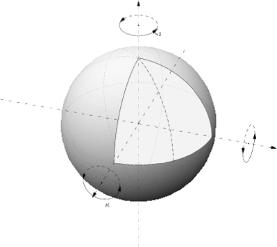
(a) $l=2$

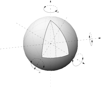
(b) $l=3$

Figure 1. Dihedral groups $D_{l}$, with the upper half of the fundamental domains in white.

Consider the permutation representation of $D_{l}$ given by left multiplication (that is, the Cayley immersion $\sigma\colon D_{l}\to\Sigma_{2l}$ of $D_{l}$ into the symmetric group on the $2l$ elements of $D_{l}$, defined by $\sigma(g)(x)=gx$ for each $g,x\in D_{l}$, see [13] for more details). The action of $D_{l}$ on $\mathbb{R}^{3}$ induces an orthogonal action on the configuration space $\mathbb{R}^{6l}$ of $n=2l$ point particles ${\bm{q}}_{i}\in\mathbb{R}^{3}$ in the three-dimensional space. The Newtonian potential for the $n$-body problem, homogeneous with degree $-\alpha$ induces by restriction on the fixed subspace $\left(\mathbb{R}^{6l}\right)^{D_{l}}\cong\mathbb{R}^{3}$ a homogeneous potential defined for each ${\bm{q}}\in\mathbb{R}^{3}$ by

((3.1)) $$U({\bm{q}})=\sum_{g\in D_{l}\smallsetminus\{1\}}\left|{\bm{q}}-g{\bm{q}}\right|^{-\alpha},$$

provided we assume (without loss of generality) all masses $m_{i}^{2}=1/l$. Now, the potential $U$ in (3.1) can be re-written in terms of coordinates ${\bm{q}}=(z,y)\in\mathbb{C}\times\mathbb{R}$ as

$$U({\bm{q}}) =\sum_{j=1}^{l-1}|{\bm{q}}-\zeta_{l}^{j}{\bm{q}}|^{-\alpha}+\sum_{j=1}^{l}|{\bm{q}}-\zeta_{l}^{j}\kappa{\bm{q}}|^{-\alpha}$$

$$=\sum_{j=1}^{l-1}|z-\zeta_{l}^{j}z|^{-\alpha}+\sum_{j=1}^{l}\left(|z-\zeta_{l}^{j}\overline{z}|^{2}+4y^{2}\right)^{-\alpha/2}.$$

By definition, for each $g\in D_{l}$, $U(g{\bm{q}})=U({\bm{q}})$. Further symmetries of $U$ are:

1. the reflection on the plane $y=0$ (given by $h\colon(z,y)\mapsto(z,-y)$),

2. the $l$ reflections on the planes containing the $l$-gonal axis and one of the digonal axes,

3. and the $l$ reflections on the planes containing the $l$-gonal axis and the points $(\zeta_{l}^{j}e^{\pi i/l},0)$, $j=1,\ldots,l$.

It is not difficult to prove that these are (up to conjugacy and multiplication with elements in $D_{l}$) all the elements of the normaliser of $D_{l}$ in $O(3)$. Thus we can study $U$ only in the left-upper area of the $D_{l}$-fundamental domain on $S^{2}\subset\mathbb{R}^{3}$, as we have seen in figures 1(a) and 1(b). Now, in order to simplify the expression of the potential we introduce the variables $r$ and $\xi$ as follows. If $y\geq 0$ and $z\neq 0$, let $r=r(z,y)$ be defined as $r=1+2y^{2}/|z|^{2}-2y/|z|\sqrt{y^{2}/|z|^{2}+1}$ and $\xi=\dfrac{\overline{z}}{z}$. Hence $r\in(0,1]$, with $r=1$ if and only if $y=0$, $1+r^{2}=r(2+4y^{2}/|z^{2}|)$ and therefore

$$|z-\zeta_{l}^{j}\overline{z}|^{2}+4y^{2} =|z|^{2}\left(|1-\zeta_{l}^{j}\dfrac{\overline{z}}{z}|^{2}+4\dfrac{y^{2}}{|z|^{2}}\right)=\dfrac{|z|^{2}}{r}\left|1-\zeta_{l}^{j}r\xi\right|^{2}.$$

In these coordinates the potential function $U({\bm{q}})$ can be written as

((3.2)) $$U=|z|^{-\alpha}\left[\sum_{j=1}^{l-1}|1-\zeta_{l}^{j}|^{-\alpha}+r^{-\alpha/2}\sum_{j=1}^{l}\left|1-\zeta_{l}^{j}r\xi\right|^{-\alpha}\right].$$

We can now state the integral representation of the potential (3.2) proven in the Appendix A (see also [2] and remark A.5 below).

3.1 Proposition.

For $\beta\in(0,1)$, $r\in(0,1]$ and $\xi\in S^{1}\subset\mathbb{C}$ the potential $U$ can be written as

$$U=|z|^{-\alpha}\left[c_{l}+lr^{-\beta}\dfrac{\sin(\beta\pi)}{\pi}\int_{0}^{1}\dfrac{(1-t)^{-\beta}t^{\beta-1}}{{(1-tr^{2})}^{\beta}}\dfrac{1-(tr)^{2l}}{|1-(tr)^{l}\xi^{l}|^{2}}\,dt\right],$$

where $c_{l}$ is the constant $c_{l}=\sum_{j=1}^{l-1}|1-\zeta_{l}^{j}|^{-\alpha}$.

Proof.

For the proof of this result, see Appendix A.∎

3.2 Remark.

The above integral representation plays a fundamental role in order to find all the central configuration. In fact, otherwise the expression of the potential given in formula (3.2) is quite difficult to deal with.

3.1. Planar type central configurations

On the unit sphere $S\subset\mathbb{R}^{3}$ (of equation $|z|^{2}+y^{2}=1$), parametrised by $(\varphi,\theta)\in(-\pi/2,\pi/2)\times[0,2\pi)$ with $y=\sin\varphi$ and $z=\cos\varphi e^{i\theta}$, the (reduced to the $2$-sphere) potential reads

((3.3)) $${U}(\theta,\varphi)\!\!=\!\!(2\cos\varphi)^{-\alpha}\left[\sum_{j=1}^{l-1}\left(\sin\dfrac{j\pi}{l}\right)^{-\alpha}\!\!\!+\!\!\sum_{j=1}^{l}\left(\sin^{2}(\dfrac{j\pi}{l}\!-\!\theta)\!+\!\tan^{2}\varphi\right)^{-\frac{\alpha}{2}}\right],$$

and by Proposition 3.1 also as

$${U}(\theta,r)=\left(\dfrac{1+r^{2}}{4r}\right)^{\beta}\left[c_{l}+lr^{-\beta}\dfrac{\sin(\beta\pi)}{\pi}I(r,\theta)\right]$$

$$\textrm{where}\ \ I(r,\theta)=\int_{0}^{1}\dfrac{(1-t)^{-\beta}t^{\beta-1}}{{(1-tr^{2})}^{\beta}}\dfrac{1-(tr)^{2l}}{1+(tr)^{2l}-2(tr)^{l}\cos(2l\theta)}\,dt,$$

with (just for $\varphi\in[0,\pi/2)$)

$$r=1+2\tan^{2}\varphi-2\dfrac{\tan\varphi}{\cos\varphi}=\dfrac{1-\sin\varphi}{1+\sin\varphi}$$

and hence

$$\sin\varphi=\dfrac{1-r}{1+r}\text{\ and \ }\cos^{2}\varphi=\dfrac{4r}{1+r^{2}}.$$

In spherical coordinates, the symmetry reflections of $U$ are (up to conjugacy)

1. the reflection on the horizontal plane: $h_{\varphi}\colon(\theta,\varphi)\mapsto(\theta,-\varphi)$,

2. the reflection on the plane containing the $l$-gonal axis and the digonal axis $h_{\theta}\colon(\theta,\varphi)\mapsto(-\theta,\varphi)$

3. and the reflection on the plane containing the $l$-gonal axis and the point $(e^{\pi i/l},0)$, defined as $h^{\prime}_{\theta}\colon(\theta,\varphi)\mapsto(\pi/l-\theta,\varphi)$.

As direct consequence of the Palais’ symmetric criticality principle, it follows that critical points of the restrictions of the reduced potential $U$ to the $1$-spheres of such fixed planes are critical points for the restriction of $U$ to the sphere, and hence are central configurations for $U$. In fact, as already observed this $1$-spheres are nothing but the spaces fixed by each of the reflections given in $(i)$, $(ii)$ and $(iii)$. In principle it can be exist other critical points for the restriction of the potential $U$ to the sphere which do not lie in these fixed spaces. However if we are able to show that out of this $1$-spheres the derivative of the potential is bounded away from zero, we have done.

Now consider the derivative with respect to $\theta$ of $U$, which by Proposition 3.1 can be written as follows

((3.4)) $$\dfrac{\partial U}{\partial\theta}=-4l^{2}\sin(2l\theta)\dfrac{(1+r^{2})^{\beta}\sin(\beta\pi)}{\pi(2r)^{\alpha}}I(r,\theta)$$

where $I(r,\theta)$ is strictly positive and defined for $(\theta,r)\neq(2k\pi/l,1)$, $k$ integer. Hence for each $r\in(0,1]$ the derivative $\dfrac{\partial U}{\partial\theta}$ is strictly negative for $\theta\in(0,\dfrac{\pi}{2l})$ and strictly positive for $\theta\in(\dfrac{\pi}{2l},\dfrac{\pi}{l})$. It is zero for $\theta=\dfrac{k\pi}{2l}$ and $r\in(0,1)$ and $\theta=\dfrac{(2k+1)\pi}{2l}$ and $r=1$. Thus, for $\varphi=0$, we have proved the following proposition:

3.3 Lemma (Planar $2l$-gon).

For any $\alpha\in(0,2)$ central configurations which are $h_{\varphi}$-symmetric are on the vertices $(e^{(2k+1)\pi i/(2l)},0)$ of the regular $2l$-gon.

3.2. Prism type central configurations

Now we have to explore the cases $\theta=k\pi/l$ and $\theta=(2k+1)\pi/(2l)$, which correspond respectively to prisms and antiprisms. The derivative of (3.3) with respect to $\varphi$ is

((3.5)) $$\dfrac{\partial U}{\partial\varphi} =2\beta\dfrac{\tan\varphi}{(2\cos\varphi)^{\alpha}}\left[c_{l}-\sum_{j=1}^{l}\dfrac{\cos^{2}(j\pi/l-\theta)}{\left(\sin^{2}(j\pi/l-\theta)+\tan^{2}\varphi\right)^{\beta+1}}\right]$$

$$=2\beta\dfrac{\tan\varphi}{(2\cos\varphi)^{\alpha}}\left[f_{\theta}(\varphi)\right].$$

The term in square brackets $f_{\theta}(\varphi)$ has the same sign of $\dfrac{\partial U}{\partial\varphi}$, and since $c_{l}$ is a constant and each term of the sum is strictly monotone in $\varphi$, for each $\theta$ the function $f_{\theta}(\varphi)$ can vanish at most once in the interval $(0,\pi/2)$. Since the limit of the sum as $\varphi\to\pi/2$ is zero and $c_{l}$ is positive, there will be a unique zero in $(0,\pi/2)$ (for a fixed $\theta$) for all the values $\theta$ such that $\lim_{\varphi\to 0}f_{\theta}(\varphi)<0$, i.e.

$$\lim_{\varphi\to 0}\sum_{j=1}^{l}\dfrac{\cos^{2}(j\pi/l-\theta)}{\left(\sin^{2}(j\pi/l-\theta)+\tan^{2}\varphi\right)^{\beta+1}}>c_{l}=\sum_{k=1}^{l-1}\left(\sin^{2}(j\pi/l)\right)^{-\beta}.$$

Now, since $\lim_{\varphi\to 0}f_{0}(\varphi)=-\infty,$ there exists a unique minimum $\hat{\varphi}$ for $\theta=k\pi/l$, $k=0\ldots 2l-1$, corresponding to a prism.

3.4 Lemma (Prisms).

There are exactly $4l$ central configurations which are $h_{\theta}$-symmetric (up to conjugacy), and they are precisely on the vertices of a prism: $(\cos\hat{\varphi}^{\prime}e^{k\pi i/l},\pm\sin\hat{\varphi}^{\prime})$.

We observe that in the dihedral four body problem these kind of central configurations collapse to square type central configurations.

3.3. Antiprism type central configurations

It is left to compute critical points for $\theta=(2k+1)\pi/(2l)$, that is, to find zeroes of $f_{\theta}(\varphi)$ for $\theta=\dfrac{\pi}{2l}$, or, equivalently, $h^{\prime}_{\theta}$-symmetric central configurations.

3.5 Lemma (Antiprisms).

There are exactly $2l$ central configurations which are $h^{\prime}_{\theta}$-symmetric (up to conjugacy) and $\varphi\neq 0$. They are on the vertices of a prism: $(\cos\hat{\varphi}e^{(2k+1)\pi i/(2l)},\pm\sin\hat{\varphi})$.

We remark that in the four body problem the antiprism type central configurations reduce to tetrahedral type configurations.

Proof.

It suffices to show that

$$\sum_{j=1}^{l}\dfrac{\cos^{2}(j\pi/l-\pi/(2l))}{\left(\sin^{2}(j\pi/l-\pi/(2l))\right)^{\beta+1}}>\sum_{k=1}^{l-1}\left(\sin^{2}(j\pi/l)\right)^{-\beta}.$$

If $\lfloor l/2\rfloor$ denotes the greatest integer $n\leq l/2$, that is

$$\lfloor l/2\rfloor=\begin{cases}(l-1)/2&\text{ $l$ odd}\\ l/2&\text{$l$ even,}\end{cases}$$

then

$$\sum_{j=1}^{l}\dfrac{\cos^{2}(j\pi/l-\pi/(2l))}{\left(\sin^{2}(j\pi/l-\pi/(2l))\right)^{\beta+1}}=2\sum_{j=1}^{\lfloor l/2\rfloor}\dfrac{\cos^{2}(j\pi/l-\pi/(2l))}{\left(\sin^{2}(j\pi/l-\pi/(2l))\right)^{\beta+1}}.$$

On the other hand

$$\sum_{j=1}^{l-1}\left(\sin^{2}(j\pi/l)\right)^{-\beta}=2\sum_{j=1}^{\lfloor l/2\rfloor}\left(\sin^{2}(j\pi/l)\right)^{-\beta}+d_{l},$$

where

$$d_{l}=\begin{cases}1&\text{$l$ even}\\ 0&\text{$l$ odd}\end{cases}$$

Now then, since

$$\dfrac{\cos^{2}x}{\left(\sin^{2}x\right)^{\beta+1}}=\dfrac{1}{\left(\sin^{2}x\right)^{\beta+1}}-\dfrac{1}{\left(\sin^{2}x\right)^{\beta}},$$

the conclusion would follow once we could prove that

$$2\sum_{j=1}^{\lfloor l/2\rfloor}C_{j}>d_{l},$$

where

$$C_{j}\!=\!\dfrac{1}{\left(\sin^{2}(j\pi/l-\pi/(2l))\right)^{\beta+1}}-\dfrac{1}{\left(\sin^{2}(j\pi/l-\pi/(2l))\right)^{\beta}}-\dfrac{1}{\left(\sin^{2}(j\pi/l)\right)^{\beta}}.$$

If $l=2$, it turns out that $C_{1}=2^{\beta}-1$ and hence $2\sum_{j=1}^{\lfloor l/2\rfloor}C_{j}=2C_{1}>0=d_{2}$. If $l=3$, then $C_{1}=2^{\alpha}(3-3^{-\beta})$, which is greater than $2$ for all $\alpha=2\beta$, so that $2C_{1}>1=d_{1}$. In general, since $j\leq l/2$, $\sin(j\pi/l)>\sin(j\pi/l-\pi/(2l))$, and therefore

$$C_{j} >\dfrac{1}{\left(\sin^{2}(j\pi/l-\pi/(2l))\right)^{\beta+1}}-\dfrac{2}{\left(\sin^{2}(j\pi/l-\pi/(2l))\right)^{\beta}}$$

$$=\dfrac{1-2\sin^{2}(j\pi/l-\pi/(2l))}{\left(\sin^{2}(j\pi/l-\pi/(2l))\right)^{\beta+1}}.$$

The first term is estimated by

$$\begin{split}C_{1}\geq\dfrac{1-2\sin^{2}(\pi/(2l))}{\left(\sin^{2}(\pi/(2l))\right)^{\beta+1}}>\dfrac{1-\dfrac{\pi^{2}}{2l^{2}}}{\left(\dfrac{\pi}{2l}\right)^{\alpha+2}}=(1-\dfrac{\pi^{2}}{2l^{2}})\dfrac{2^{\alpha+2}l^{\alpha+2}}{\pi^{\alpha+2}}\\ \geq\dfrac{4l^{2}}{\pi^{2}}-2>\dfrac{l^{2}}{4}-2,\end{split}$$

and all other terms $C_{j}$ with $j\geq 2$ are in any case greater than $-1$; thus for $l\geq 4$

$$\sum_{j=1}^{\lfloor l/2\rfloor}C_{j}>C_{1}-(\lfloor\dfrac{l}{2}\rfloor-1)\geq C_{1}-\dfrac{l}{2}+1\geq\dfrac{l^{2}}{4}-\dfrac{l}{2}-1\geq 1,$$

and thus for all $l\geq 4$ we have $2\sum_{j=1}^{\lfloor l/2\rfloor}C_{j}\geq 2>d_{l},$ which concludes the proof. ∎

Since there are no other central configurations, by (3.4), we can summarise the results in the following proposition.

3.6 Proposition.

All central configurations in the dihedral $2n$-body problem are symmetric for one of the three types of reflections $h_{\varphi}$ Lemma 3.3, $h_{\theta}$ Lemma 3.4 or $h^{\prime}_{\theta}$ Lemma 3.5. They are represented in the (upper-half) fundamental domain on the sphere in figure 2.

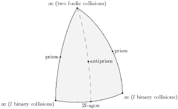
Figure 2. Central configurations in the upper-half fundamental domain.

In fact, in figure 2 it is drawn a geodesic triangle which represents the fundamental domain on the shape sphere for the dihedral $n$-body problem. In this figure are shown the three types of central configurations arising in the problem we are dealing with in the exact location together with. Moreover we observe that due to the symmetry constraint only two types of collisions can occur. We denoted by the name $l$-adic collision and binary collision, meaning that in the first case two clusters of $l$-bodies simultaneously collide, while in the second case $l$ clusters of 2 bodies simultaneously collide. This two types of collisions are all located on the same plane containing the planar central configurations while the $l$-adic central configurations can be represented in the north and south pole of the shape sphere.

Now consider equations (2.6) in coordinates $(\theta,\varphi)$ on the sphere: we set $w_{1}$ and $w_{2}$ such that ${\bm{w}}=w_{1}\dfrac{\partial{\bm{s}}}{\partial\theta}+w_{2}\dfrac{\partial{\bm{s}}}{\partial\varphi}$, i.e. (since ${\bm{s}}=(\cos\varphi e^{i\theta},\sin\varphi)$),

$${\bm{w}}=w_{1}(i\cos\varphi e^{i\theta},0)+w_{2}(-\sin\varphi e^{i\theta},\cos\varphi).$$

Then

$$\left\|{\bm{w}}\right\|=w_{1}^{2}\cos^{2}\varphi+w_{2}^{2}$$

and

$$\nabla_{{\bm{s}}}U({\bm{s}})=\dfrac{1}{\cos^{2}\varphi}\dfrac{\partial U}{\partial\theta}\dfrac{\partial{\bm{s}}}{\partial\theta}+\dfrac{\partial U}{\partial\varphi}\dfrac{\partial{\bm{s}}}{\partial\varphi}.$$

Also, equations (2.6) become

((3.6)) $$\left\{\begin{aligned} v^{\prime}&=w_{1}^{2}\cos^{2}\varphi+w_{2}^{2}+\beta v^{2}-\alpha U(\theta,\varphi)\\ \theta^{\prime}&=w_{1}\\ \varphi^{\prime}&=w_{2}\\ w_{1}^{\prime}&=(\beta-1)vw_{1}+2\tan\varphi~{}w_{1}w_{2}+\dfrac{1}{\cos^{2}\varphi}\dfrac{\partial U}{\partial\theta}\\ w_{2}^{\prime}&=(\beta-1)vw_{2}-\dfrac{1}{2}w_{1}^{2}\sin 2\varphi+\dfrac{\partial U}{\partial\varphi}.\end{aligned}\right.$$

The linearization at equilibrium points (central configurations) (2.7) is represented by the $5\times 5$ matrix $L$

$$L=\begin{bmatrix}2\beta v&0&0&0&0\\ 0&0&0&1&0\\ 0&0&0&0&1\\ 0&\dfrac{1}{\cos^{2}\varphi}\dfrac{\partial^{2}U}{\partial\theta^{2}}&\dfrac{\partial^{2}U}{\partial\theta\partial\varphi}&(\beta-1)v&0\\ 0&\dfrac{\partial^{2}U}{\partial\varphi\partial\theta}&\dfrac{\partial^{2}U}{\partial\varphi^{2}}&0&(\beta-1)v\\ \end{bmatrix}.$$

Thus the eigenvalues of the linearization can be computed in terms of the eigenvalues of the Hessian $D^{2}U(\overline{\bm{s}})$ of $U(\theta,\varphi)$:

3.7 Proposition.

The eigenvalues of $L$, at a central configuration $\overline{\bm{s}}$ (i.e. at the point $(\overline{v},\overline{\bm{s}},\bm{0})$, where $\overline{v}=\pm\sqrt{2U(\overline{\bm{s}})}$), are equal to the roots $\lambda$ of the equation

$$\lambda^{2}+(1-\beta)\overline{v}\lambda=\gamma$$

for each $\gamma$ eigenvalue of the Hessian $D^{2}U(\overline{\bm{s}})$.

By elementary calculations it follows from Proposition 3.7 that the equilibrium points $(\pm\sqrt{2U(\overline{\bm{s}})},\overline{\bm{s}},\bm{0})$ are hyperbolic when the Hessian $D^{2}U$ is non-singular at $\overline{{\bm{s}}}$, and that for each positive eigenvalue $\gamma>0$ of $D^{2}U$ there is a pair of real eigenvalues of $L$, $\lambda_{1}>0$, $\lambda_{2}<0$; for each negative eigenvalue $\gamma<0$ of $D^{2}U$, there are two eigenvalues $\lambda_{1}$, $\lambda_{2}$ of $L$ with negative real part ($\lambda_{1}$, $\lambda_{2}$ are real if $d=(1-\beta)^{2}{\overline{v}}^{2}+4\gamma>0$ and $\lambda_{1}=\lambda_{2}$ if $d=0$).

3.8 Proposition.

All equilibrium points of (3.6) are hyperbolic.

Proof.

We just need to proof that the Hessian $D^{2}U$ is non-singular at $\overline{\bm{s}}$, if ${\bm{s}}$ is a central configuration. Since each central configuration ${\bm{s}}$ lies in the line fixed by a reflection (which is a symmetry of $U$), the matrix $D^{2}U$ is diagonal at $\overline{\bm{s}}$. So the result follows once we prove that $\dfrac{\partial^{2}U}{\partial\theta^{2}}(\overline{\bm{s}})\neq 0\neq\dfrac{\partial^{2}U}{\partial\varphi^{2}}(\overline{\bm{s}})$. But by (3.4), since $I(r,\theta)$ is strictly positive and regular in a neighbourhood of $\overline{s}$, $\dfrac{\partial^{2}U}{\partial\theta^{2}}(\overline{\bm{s}})\neq 0$. By (3.5), the same holds for $\dfrac{\partial^{2}U}{\partial\varphi^{2}}(\overline{\bm{s}})$. ∎

3.9 Proposition.

The dimension of the stable (unstable) manifold of $(\overline{v},\overline{\bm{s}},\bm{0})$ with $\overline{v}=\sqrt{2U(\overline{\bm{s}})}>0$ is 3 (2) if $\overline{\bm{s}}$ is a $2l$-gon or a prism; it is 2 (3) if $\overline{\bm{s}}$ is an antiprism. The dimension of the stable (unstable) manifold of the point $(-\overline{v},\overline{\bm{s}},\bm{0})$ with $\overline{v}=\sqrt{2U(\overline{\bm{s}})}>0$ is equal to the dimension of the unstable (stable) manifold of $(\overline{v},\overline{\bm{s}},\bm{0})$. The intersection of the stable (unstable) manifold of $(\overline{v},\overline{\bm{s}},\bm{0})$ with the parabolic manifold $P$ has codimension 0 (1) in $P$ if $\overline{v}>0$. It has codimension 1 (0) in $P$ if $\overline{v}<0$.

Proof.

These facts follow directly from the stable/unstable manifold theorem and the above arguments on eigenvalues of $L$. The results are summarised in table 1. ∎

	$\overline{v}$	$\dim W^{s}$	$\dim W^{u}$	$\dim W^{s}\cap P$	$\dim W^{u}\cap P$
$2l$-gon and prism	$>0$	3	2	3	1
	$<0$	2	3	1	3
anti-prism	$>0$	2	3	2	2
	$<0$	3	2	2	2

Table 1. Dimensions of stable and unstable manifolds.

Appendix A An integral representation for $U$

The aim of this section is to give a direct proof of the integral representation for the potential $U$ used before in order to compute all the central configurations.

For $l\geq 2$, let $\widehat{P}_{l}$ denote the $l$-adic Perron-Frobenius operator, defined on complex functions $f\colon S^{1}\subset\mathbb{C}\to\mathbb{C}$ by

$$\forall\xi=e^{i\theta}\in S^{1},\widehat{P}_{l}(f)(\xi) =\dfrac{1}{l}\sum_{y\,:\,y^{l}=\xi}f(y)=\dfrac{1}{l}\sum_{j=0}^{l-1}f(e^{\frac{i(\theta+2j\pi)}{l}}).$$

For each $k\in\mathbb{Z}$,

((1.1)) $$\widehat{P}_{l}(\xi^{k})(\xi)=\dfrac{1}{l}\sum_{y\,:\,y^{l}=\xi}y^{k}=\begin{cases}\xi^{k/l}&\text{if $k\equiv 0\mod l$}\\ 0&\text{if $k\not\equiv 0\mod l$.}\end{cases}$$

In terms of the $l$-adic Perron-Frobenius operator, the potential (3.2) can be written as

((1.2)) $$U=|z|^{-\alpha}\left[c_{l}+r^{-\alpha/2}l\widehat{P}_{l}\left(\left|1-r\xi\right|^{-\alpha}\right)(\xi^{l})\right],$$

where $c_{l}$ is the constant $c_{l}=\sum_{j=1}^{l-1}|1-\zeta_{l}^{j}|^{-\alpha}$ and $\widehat{P}_{l}\left(\left|1-r\xi\right|^{-\alpha}\right)(\xi^{l})$ denotes the function $\widehat{P}_{l}\left(\left|1-r\xi\right|^{-\alpha}\right)$ of argument $\xi$ evaluated at $\xi^{l}$. In order to compute $\widehat{P}_{l}\left(\left|1-r\xi\right|^{-\alpha}\right)$, we expand $|1-r\xi|^{-\alpha}$ in a double power series as follows.

A.1 Lemma.

For each $r\in(0,1]$ and $\alpha=2\beta>0$

$$|1-r\xi|^{-\alpha}=\sum_{n=-\infty}^{+\infty}b_{n}\xi^{n},$$

with, for each $n\geq 0$,

$$b_{n}=b_{-n}=\dfrac{\sin(\beta\pi)}{\pi}r^{n}\int_{0}^{1}(1-t)^{-\beta}t^{\beta-1}t^{n}{(1-tr^{2})}^{-\beta}\,dt.$$

Proof.

$$\begin{aligned} |1-r\xi|^{-\alpha}&=(1-r\xi)^{-\beta}(1-r\xi^{-1})^{-\beta}\\ &=\left(\sum_{k=0}^{\infty}\binom{-\beta}{k}(-r\xi)^{k}\right)\cdot\left(\sum_{h=0}^{\infty}\binom{-\beta}{h}(-r\xi^{-1})^{h}\right)\\ &=\sum_{h,k=0}^{\infty}\binom{-\beta}{k}\binom{-\beta}{h}(-r)^{k+h}\xi^{k-h}\\ &=\sum_{n=-\infty}^{\infty}\underbrace{\left((-1)^{n}\sum_{\begin{subarray}{c}k-h=n\\ k,h\geq 0\end{subarray}}\binom{-\beta}{k}\binom{-\beta}{h}r^{k+h}\right)}_{b_{n}}\xi^{n}\end{aligned}.$$

Now, recall that for each $\beta>0$ and $N$ integer

$$\binom{-\beta}{N}=(-1)^{N}\binom{N+\beta-1}{N} =(-1)^{N}\dfrac{\Gamma(N+\beta)\Gamma(1-\beta)}{\Gamma(N+1)\Gamma(\beta)\Gamma(1-\beta)}$$

$$=\dfrac{(-1)^{N}}{\Gamma(\beta)\Gamma(1-\beta)}\cdot\dfrac{\Gamma(N+\beta)\Gamma(1-\beta)}{\Gamma(N+1)}$$

$$=\dfrac{(-1)^{N}\sin(\beta\pi)}{\pi}\cdot B(1-\beta,N+\beta)$$

where $B(x,y)$ denotes the beta function, defined as

$$B(x,y)=\int_{0}^{1}t^{x-1}(1-t)^{y-1}\,dt=\dfrac{\Gamma(x)\Gamma(y)}{\Gamma(x+y)}$$

and we have used the equalities

$$\Gamma(\beta)\Gamma(1-\beta)=\dfrac{\pi}{\sin(\beta\pi)},$$

$$\binom{-\beta}{N}=\dfrac{(-\beta)(-\beta-1)\ldots(-\beta-N+1)}{N!}=(-1)^{N}\dfrac{\Gamma(N+\beta)}{\Gamma(N+1)\Gamma(\beta)}$$

and

$$\binom{\beta}{N}=\dfrac{\Gamma(\beta+1)}{\Gamma(N+1)\Gamma(\beta-N+1)}.$$

We can now use the integral representation of the binomial function

((1.3)) $$\binom{-\beta}{N}=(-1)^{N}\dfrac{\sin(\beta\pi)}{\pi}\int_{0}^{1}(1-t)^{-\beta}t^{\beta-1}t^{N}\,dt,$$

which implies that, by setting $N=h+n$,

$$b_{n} =(-1)^{n}\sum_{h=0}^{\infty}\left((-1)^{n+h}\dfrac{\sin(\beta\pi)}{\pi}\int_{0}^{1}(1-t)^{-\beta}t^{\beta-1}t^{n+h}\,dt\binom{-\beta}{h}r^{n+2h}\right)$$

$$=\dfrac{\sin(\beta\pi)}{\pi}r^{n}\sum_{h=0}^{\infty}\left((-1)^{h}\int_{0}^{1}(1-t)^{-\beta}t^{\beta-1}t^{n+h}\,dt\binom{-\beta}{h}r^{2h}\right)$$

$$=\dfrac{\sin(\beta\pi)}{\pi}r^{n}\int_{0}^{1}(1-t)^{-\beta}t^{\beta-1}t^{n}\sum_{h=0}^{\infty}\underbrace{\left((-1)^{h}t^{h}\binom{-\beta}{h}r^{2h}\right)}_{\binom{-\beta}{h}(-tr^{2})^{h}}\,dt$$

$$=\dfrac{\sin(\beta\pi)}{\pi}r^{n}\int_{0}^{1}(1-t)^{-\beta}t^{\beta-1}t^{n}{(1-tr^{2})}^{-\beta}\,dt.$$

∎

A.2 Lemma.

For each $\beta\in(0,1)$, $r\in(0,1]$ and integer $l\geq 2$

$$\widehat{P}_{l}\left(|1-r\xi|^{-\alpha}\right)=\sum_{n=-\infty}^{+\infty}b_{ln}\xi^{n}.$$

Proof.

It follows directly from equation (1.1). The convergence is easy to check. ∎

A.3 Lemma.

For each $\beta\in(0,1)$ and $r\in(0,1]$ and integer $l\geq 2$

$$\widehat{P}_{l}\left(|1-r\xi|^{-\alpha}\right)=\dfrac{\sin(\beta\pi)}{\pi}\int_{0}^{1}\dfrac{(1-t)^{-\beta}t^{\beta-1}}{{(1-tr^{2})}^{\beta}}\dfrac{1-(tr)^{2l}}{|1-(tr)^{l}\xi|^{2}}\,dt.$$

Proof.

$$\widehat{P}_{l}\left(|1-r\zeta|^{-\alpha}\right) =\sum_{n=-\infty}^{\infty}b_{ln}\zeta^{n}=\sum_{n=0}^{\infty}b_{ln}\zeta^{n}+\sum_{n=1}^{\infty}b_{ln}\zeta^{-n}$$

$$=\!\!\!\sum_{n=0}^{\infty}\left(\dfrac{\sin(\beta\pi)}{\pi}r^{ln}\int_{0}^{1}(1-t)^{-\beta}t^{\beta-1}t^{ln}{(1-tr^{2})}^{-\beta}\,dt\right)\zeta^{n}\!+$$

$$+\!\!\!\sum_{n=1}^{\infty}\left(\dfrac{\sin(\beta\pi)}{\pi}r^{ln}\int_{0}^{1}(1-t)^{-\beta}t^{\beta-1}t^{ln}{(1-tr^{2})}^{-\beta}\,dt\right)\zeta^{-n}$$

$$=\!\!\!\dfrac{\sin(\beta\pi)}{\pi}\!\!\int_{0}^{1}\!\!\dfrac{(1-t)^{-\beta}t^{\beta-1}}{{(1-tr^{2})}^{\beta}}\left[\sum_{n=0}^{\infty}(tr)^{ln}\zeta^{n}\!\!+\!\!\sum_{n=1}^{\infty}(tr)^{ln}\zeta^{-n}\right]\!\!dt.$$

The conclusion follows since

$$\sum_{n=0}^{\infty}(tr)^{ln}\zeta^{n}+\sum_{n=1}^{\infty}(tr)^{ln}\zeta^{-n}=\dfrac{1-(tr)^{2l}}{|1-(tr)^{l}\zeta|^{2}}.$$

∎

Thus we proved the following result.

A.4 Proposition.

For $\beta\in(0,1)$, $r\in(0,1]$ and $\xi\in S^{1}\subset\mathbb{C}$ the potential $U$ can be written as

$$U=|z|^{-\alpha}\left[c_{l}+lr^{-\beta}\dfrac{\sin(\beta\pi)}{\pi}\int_{0}^{1}\dfrac{(1-t)^{-\beta}t^{\beta-1}}{{(1-tr^{2})}^{\beta}}\dfrac{1-(tr)^{2l}}{|1-(tr)^{l}\xi^{l}|^{2}}\,dt\right],$$

where $c_{l}$ is the constant $c_{l}=\sum_{j=1}^{l-1}|1-\zeta_{l}^{j}|^{-\alpha}$.

A.5 Remark.

An analogue of the integral representation of the potential is well known, and can be traced back to F.-F. Tisserand’s book [23] (chapter XVII) for the exponent $\alpha=1$; it had been used by M. Lindow [16] (section 3) in computing central configurations for the planar gravitational field generated by a regular $n$-gon. More recently D. Bang and B. Elmabsout extended and generalised Lindow’s theorem, proving an equivalent of 3.1 (Proposition 7 and 8 of [2]). The proof given here is direct, and allows explicit estimates that can be used to compute the Hessian for the potential restricted to the shape sphere. Furthermore, it involves an interesting connection with the $l$-adic Ruelle–Perron–Frobenius operator (see P. Gaspard’s paper [15]), which is worth a mention.

References

- [1] Ambrosetti, A., and Coti Zelati, V. Non-collision periodic solutions for a class of symmetric -body type problems. Topol. Methods Nonlinear Anal. 3, 2 (1994), 197–207.
- [2] Bang, D., and Elmabsout, B. Representations of complex functions, means on the regular -gon and applications to gravitational potential. J. Phys. A 36, 45 (2003), 11435–11450.
- [3] Barutello, V., Ferrario, D. L., and Terracini, S. Symmetry groups of the planar -body problem and action–minimizing trajectories. Arch. Rational Mech. Anal. (2007). to appear.
- [4] Chen, K.-C. Binary decompositions for planar -body problems and symmetric periodic solutions. Arch. Ration. Mech. Anal. 170, 3 (2003), 247–276.
- [5] Chen, K.-C. Variational methods on periodic and quasi-periodic solutions for the -body problem. Ergodic Theory Dynam. Systems 23, 6 (2003), 1691–1715.
- [6] Chenciner, A. Action minimizing solutions of the Newtonian -body problem: from homology to symmetry. In Proceedings of the International Congress of Mathematicians, Vol. III (Beijing, 2002) (Beijing, 2002), Higher Ed. Press, pp. 279–294.
- [7] Chenciner, A., and Montgomery, R. A remarkable periodic solution of the three-body problem in the case of equal masses. Ann. of Math. (2) 152, 3 (2000), 881–901.
- [8] Chenciner, A., and Venturelli, A. Minima de l’intégrale d’action du problème newtonien de 4 corps de masses égales dans : orbites “hip-hop”. Celestial Mech. Dynam. Astronom. 77, 2 (2000), 139–152 (2001).
- [9] Delgado, J., and Vidal, C. The tetrahedral -body problem. J. Dynam. Differential Equations 11, 4 (1999), 735–780.
- [10] Devaney, R. L. Triple collision in the planar isosceles three-body problem. Invent. Math. 60, 3 (1980), 249–267.
- [11] Devaney, R. L. Singularities in classical mechanical systems. In Ergodic theory and dynamical systems, I (College Park, Md., 1979–80), vol. 10 of Progr. Math. Birkhäuser Boston, Mass., 1981, pp. 211–333.
- [12] Ferrario, D. L. Symmetry groups and non-planar collisionless action-minimizing solutions of the three-body problem in three-dimensional space. Arch. Rational Mech. Anal. 179 (2006), 389–412.
- [13] Ferrario, D. L. Transitive decomposition of symmetry groups for the -body problem. Adv. in Math. 2 (2007), 763–784.
- [14] Ferrario, D. L., and Terracini, S. On the existence of collisionless equivariant minimizers for the classical n-body problem. Invent. Math. 155, 2 (2004), 305–362.
- [15] Gaspard, P. -adic one-dimensional maps and the Euler summation formula. J. Phys. A 25, 8 (1992), L483–L485.
- [16] Lindow, M. Der kreisfall im problem der körper. Astron. Nach. 228, 5461 (1924), 234–248.
- [17] McGehee, R. Triple collision in the collinear three-body problem. Invent. Math. 27 (1974), 191–227.
- [18] Moeckel, R. Orbits of the three-body problem which pass infinitely close to triple collision. Amer. J. Math. 103, 6 (1981), 1323–1341.
- [19] Moeckel, R. Orbits near triple collision in the three-body problem. Indiana Univ. Math. J. 32, 2 (1983), 221–240.
- [20] Salomone, M., and Xia, Z. Non-planar minimizers and rotational symmetry in the -body problem. J. Differential Equations 215, 1 (2005), 1–18.
- [21] Simó, C., and Lacomba, E. Analysis of some degenerate quadruple collisions. Celestial Mech. 28, 1-2 (1982), 49–62.
- [22] Sundman, K. F. Nouvelles recherches sur le probleme des trois corps. Acta Soc. Sci. Fenn. 35, 9 (1909).
- [23] Tisserand, F.-F. Traité de mécanique céleste. Gauthiers-Villars, Paris, 1889. Tome I (Reprinted by Jacques Gabay in 1990).
- [24] Vidal, C. The tetrahedral -body problem with rotation. Celestial Mech. Dynam. Astronom. 71, 1 (1998/99), 15–33.