Mutual information in random Boolean models of regulatory networks

Abstract

The amount of mutual information contained in time series of two elements gives a measure of how well their activities are coordinated. In a large, complex network of interacting elements, such as a genetic regulatory network within a cell, the average of the mutual information over all pairs $\langle I\rangle$ is a global measure of how well the system can coordinate its internal dynamics. We study this average pairwise mutual information in random Boolean networks (RBNs) as a function of the distribution of Boolean rules implemented at each element, assuming that the links in the network are randomly placed. Efficient numerical methods for calculating $\langle I\rangle$ show that as the number of network nodes $N$ approaches infinity, the quantity $N\langle I\rangle$ exhibits a discontinuity at parameter values corresponding to critical RBNs. For finite systems it peaks near the critical value, but slightly in the disordered regime for typical parameter variations. The source of high values of $N\langle I\rangle$ is the indirect correlations between pairs of elements from different long chains with a common starting point. The contribution from pairs that are directly linked approaches zero for critical networks and peaks deep in the disordered regime.

I Introduction

The dynamical behavior of a large, complex network of interacting elements is generally quite difficult to understand in detail. One often has only partial information about the interactions involved and the presence of multiple influences on each element can give rise to exceedingly complicated dynamics even in fully deterministic systems. A paradigmatic case is the network of genes within a cell, where the interactions correspond to transcriptional (and post-transcriptional) regulatory mechanisms. The expression of a single gene may be subject to regulation by itself and up to 15–20 proteins derived from other genes, and the network of such interactions has a complicated structure, including positive and negative feedback loops and nontrivial combinatorial logic. In this paper we study mutual information (defined below) a measure of the overall level of coordination achieved in models of complex regulatory networks. We find a surprising discontinuity in this measure for infinite systems as parameters are varied. We also provide heuristic explanations of the infinite system results, the influence of noise, and finite size effects.

The theory of the dynamics of such complicated networks begins with the study of the simplest model systems rich enough to exhibit complex behaviors: Random Boolean Networks (RBNs). In a RBN model, each gene (or “node”) $g$ is represented as a Boolean logic gate that receives inputs from some number $k_{g}$ other genes. The RBN model takes the network to be drawn randomly from an ensemble of networks in which (i) the inputs to each gene are chosen at random from among all of the genes in the system; and (ii) the Boolean rule at $g$ is selected at random from a specified distribution over all possible Boolean rules with $k_{g}$ inputs. These two assumptions of randomness permit analytical insights into the typical behavior of a large network.

One important feature of RBNs is that their dynamics can be classified as ordered, disordered, or critical. In “ordered” RBNs, the fraction of genes that remain dynamical after a transient period vanishes like $1/N$ as the system size $N$ goes to infinity; almost all of the nodes become “frozen” on an output value (0 or 1) that does not depend on the initial state of the network Samuelsson and Socolar (2006). In this regime the system is strongly stable against transient perturbations of individual nodes. In “disordered” (or “chaotic”) RBNs, the number of dynamical, or “unfrozen” nodes scales like $N$ and the system is unstable to many transient perturbations Samuelsson and Socolar (2006).

For present purposes, we consider ensembles of RBNs parametrized by the average indegree $K$ (i.e., average number of inputs to the nodes in the network), and the bias $p$ in the choice of Boolean rules. The indegree distribution is Poissonian with mean $K$ and at each node the rule is constructed by assigning the output for each possible set of input values to be $1$ with probability $p$, with each set treated independently. If $p=0.5$, the rule distribution is said to be unbiased. For a given bias, the critical connectivity, $K_{\textrm{c}}$, is equal to Derrida and Pomeau (1986):

$$K_{\textrm{c}}=[2p(1-p)]^{-1}.$$ (1)

For $K<K_{\textrm{c}}$ the ensemble of RBNs is in the ordered regime; for $K>K_{\textrm{c}}$, the disordered regime. For $K=K_{\textrm{c}}$, the ensemble exhibits critical scaling of the number of unfrozen nodes; e.g., the number of unfrozen nodes scales like $N^{2/3}$. The order-disorder transition in RBNs has been characterized by several quantities, including fractions of unfrozen nodes, convergence or divergence in state space, and attractor lengths Aldana-Gonzalez et al. (2003).

It is an attractive hypothesis that cell genetic regulatory networks are critical or perhaps slightly in the ordered regime Kauffman (1990); Stauffer (1994). Critical networks display an intriguing balance between robust behavior in the presence of random perturbations and flexible switching induced by carefully targeted perturbations. That is, a typical attractor of a critical RBN is stable under the vast majority of small, transient perturbations (flipping one gene to the “wrong” state and then allowing the dynamics to proceed as usual), but there are a few special perturbations that can lead to a transition to a different attractor. This observation forms the conceptual basis for thinking of cell types as attractors of critical networks, since cell types are both homeostatic in general and capable of differentiating when specific signals (perturbations) are delivered.

Recently, some experimental evidence has been shown to support the idea that genetic regulatory networks in eukaryotic cells are dynamically critical. In Ref. Shmulevich et al. (2005), the microarray patterns of gene activities of HeLa cells were analyzed, and the trajectories in a HeLa microarray time-series data characterized using a Lempel-Ziv complexity measure on binarized data. The conclusion was that cells are either ordered or critical, not disordered. In Ref. Rämö et al. (2006), it was deduced that deletion of genes in critical networks should yield a power law distribution of the number of genes that alter their activities with an exponent of $-1.5$ and observed data on 240 deletion mutants in yeast showed this same exponent. And in Ref. Serra et al. (2004), micro-array gene expression data following silencing of a single gene in yeast was analyzed. Again, the data suggests critical dynamics for the gene regulatory network. These results suggest that operation at or near criticality confers some evolutionary advantage.

In this paper we consider a feature that quantifies the sense in which critical networks are optimal choices within the class of synchronously updated RBNs. We study a global measure of the propagation of information in the network, the average pairwise mutual information, and show that it takes its optimal value on the ensemble of critical networks. Thus, within the limits of the RBN assumptions of random structure and logic, the critical networks enable information to be transmitted most efficiently to the greatest number of network elements.

The average pairwise mutual information is defined as follows. Let $s_{a}$ be a process that generates a $0$ with probability $p_{0}$ and a $1$ with probability $p_{1}$. We define the entropy of $s_{a}$ as

$$H[s_{a}]\equiv-p_{0}\log_{2}p_{0}-p_{1}\log_{2}p_{1}.$$ (2)

Similarly, for a process $s_{ab}$ that generates pairs $xy$ with probabilities $p_{xy}$, where $x,y\in\{0,1\}$, we define the joint entropy as

$$H[s_{ab}] \equiv-p_{00}\log_{2}p_{00}-p_{01}\log_{2}p_{01}$$

$$-p_{10}\log_{2}p_{10}-p_{11}\log_{2}p_{11}.$$ (3)

For a particular RBN, we imagine running the dynamics for infinitely long times and starting from all possible initial configurations. The fraction of time steps for which the value of node $i$ is $x$ gives $p_{x}$ for the process $s_{i}$. The value of $p_{xy}$ for the process $s_{ij}$ is given by the fraction of time steps for which node $i$ has the value $x$ and on the next time step node $j$ has the value $y$. The mutual information of the pair $ij$ is

$$M_{ij}=H[s_{i}]+H[s_{j}]-H[s_{ij}].$$ (4)

With this definition, $M_{ij}$ measures the extent to which information about node $i$ at time $t$ influences node $j$ one time step later. Note that the propagation may be indirect; a nonzero $M_{ij}$ can result when $i$ is not an input to $j$ but both are influenced by a common node through previous time steps.

To quantify the efficiency of information propagation through the entire network, we define the average pairwise mutual information for an ensemble of networks to be

$$\langle I\rangle=\biggl{\langle}N^{-2}\sum_{i,j}M_{ij}\biggr{\rangle},$$ (5)

where $\langle\cdot\rangle$ indicates an average over members of the ensemble. It has previously been observed that $\langle I\rangle$ is maximized near the critical regime in numerical simulations of random Boolean networks with a small number of nodes (less than 500) Ribeiro et al. (2006).

In general, one does not expect a given element to be strongly correlated with more than a few other elements in the network, so the number of pairs $ij$ that contribute significantly to the sum in Eq. (5) is expected to be at most of order $N$. It is therefore convenient to work with the quantity ${\cal I}_{N}\equiv N\langle I\rangle$, which may approach a nonzero constant in the large $N$ limit. We use the symbol ${\cal I}_{\infty}$ to denote the $N\rightarrow\infty$ limit of ${\cal I}_{N}$.

As an aside, we note that other authors have considered different information measures and found optimal behavior for critical Boolean networks. Krawitz and Shmulevich have found that “basin entropy,” which characterizes the number and sizes of basins of attraction and hence the ability of the system to respond differently to different inputs, is maximized for critical networks Krawitz and Shmulevich (2007). Luque and Ferrera have studied the self-overlap Luque and Ferrera (2000), which differs from $\langle I\rangle$ in that it involves comparison of each node to its own state one time step later (not to the state of another node that might be causally connected to it) and that the average over the network is done before calculating the mutual information. Bertschinger and Natschläger have introduced the “network-mediated separation” ($NM$-separation) in systems where all nodes are driven by a common input signal, finding that critical networks provide maximal $NM$-separation for different input signals Bertschinger and Natschläger (2004). Our definition of $\langle I\rangle$ places the focus on the autonomous, internal dynamics of the network and the transmission of information along links, which allows for additional insights into the information flow.

Two simple arguments immediately show that ${\cal I}_{\infty}$ is zero both in the ordered regime and deep in the disordered regime. First, note that $M_{ij}=0$ whenever $s_{i}$ or $s_{j}$ generates only 0s or only 1s. In the ordered regime, where almost all nodes remain frozen on the same value on all attractors, the number of nonzero elements $M_{ij}$ remains bounded for large $N$. Thus $\langle I\rangle$ must be of order $N^{-2}$ and ${\cal I}_{\infty}=0$ everywhere in the ordered regime.

Second, if $s_{ij}$ is the product of two independent processes $s_{i}$ and $s_{j}$, then $M_{ij}=0$. This occurs for every pair of connected nodes in the limit of strong disorder, where $K$ is very large and the Boolean rules are drawn from uniformly weighted distributions over all possible rules with $k_{g}$ inputs. The correlation between the output of a node and any particular one of its inputs becomes vanishingly small because there are many combinations of the other inputs, each producing a randomly determined output value, so the probability for the output to be 1 is close to $p$ for either value of the given input. ${\cal I}_{\infty}$ therefore vanishes in the limit of large $K$.

Given that ${\cal I}_{\infty}=0$ for all network parameters that yield ordered ensembles, one might expect that it rises to a maximum somewhere in the disordered regime before decaying back to zero in the strong disorder limit. We show below that this is not the case. Fixing the bias parameter $p$ at $1/2$ and allowing the average indegree $K$ to vary, we find that ${\cal I}_{\infty}$ exhibits a jump discontinuity at the critical value $K=2$, then decays monotonically to zero as $K$ is increased. The conclusion is that among ensembles of unbiased RBNs, average pairwise mutual information is maximized for critical ensembles.

We begin by presenting analytic arguments and numerical methods for investigating the large system limit and establishing the existence of a discontinuity at $K=2$ and monotonic decay for $K>2$. We then present results from numerical experiments obtained by averaging over $10^{4}$ instances of networks of sizes up to $N=1000$. These data show a strong peak near the critical value $K=2$, as expected from the analysis. Interestingly, the peak is substantially higher than the size of the jump discontinuity, which may indicate that ${\cal I}_{\infty}$ for $K=2$ is an isolated point larger than $\lim_{K\rightarrow 2^{+}}{\cal I}_{\infty}$. Finally, we present numerical results on the variation of ${\cal I}_{N}$ with $p$ at fixed $K$, which again shows a peak for critical parameter values.

II Average pairwise mutual information in large networks

II.1 Mean-field calculation of ${\cal I}_{\infty}$

Mean-field calculations are commonly used in the theory of random Boolean networks. The most common forms of mean-field calculations are within the realm of the so called annealed approximation. In the annealed approximation, one assumes that the rules and the inputs are randomized at each time step. This approach is sufficient, for example, for calculating the average number of nodes that change value at each time step.

For understanding the propagation of information, a slightly more elaborate mean-field model is needed. This mean-field model is based on the assumption that the state of a node in a large disordered network is independent of its state at the previous time step, but that its rule remains fixed. In this model, each node takes the value $1$ with a given probability $b$, which we refer to as the local bias. In the annealed approximation all local biases are equal because the rules and the inputs are redrawn randomly at each time step, so the system is characterized by a single global bias. In our extended mean-field model, we consider a distribution of local biases. To determine ${\cal I}_{\infty}$, we determine the distribution of $b$, then use it to analyze the simple feed forward structures that provide the nonvanishing contributions to ${\cal I}_{\infty}$ in the disordered regime.

II.2 The distribution of local biases

An important feature characterizing the propagation of information in a network is the distribution of local biases. The local bias at a given node is determined by the rule at that node and the local biases of its inputs. Roughly speaking, when the bias of the output value is stronger than the bias of the inputs, information is lost in transmission through the node. The local bias distribution is defined as the self-consistent distribution obtained as the limit of a convergent iterative process.

Let $B_{t}$ be the stochastic function that at each evaluation returns a sample $b$ from the local bias distribution at time $t$. Then, a sample $b^{\prime}$ from $B_{t+1}$ can be obtained as follows. Let $r$ be a Boolean rule drawn from the network’s rule distribution $R$ and let $k$ denote the number of inputs to $r$. Furthermore, let $\{b_{1},\ldots,b_{k}\}$ be a set of $k$ independent samples from $B_{t}$. The sample $b^{\prime}$ is then given by

$$b^{\prime} =\sum_{\bm{\sigma}\in\{0,1\}^{k}}r(\bm{\sigma})\prod_{i=1}^{k}[\sigma_{i}b_{i}+(1-\sigma_{i})(1-b_{i})]~{}.$$ (6)

Repeated sampling of the rule $r$ and the values $b_{i}$ produces samples $b^{\prime}$ that define the distribution $B_{t+1}$. The sequence of distributions $B_{0},B_{1},B_{2},\ldots$ is initiated by $B_{0}$ that always returns $1/2$.

For many rule distributions $R$, $P(B_{t}\leq x)$ converges as $t\rightarrow\infty$. For such rule distributions, we define $B^{*}$ as the stochastic function that satisfies

$$P(B^{*}\leq x) =\lim_{t\rightarrow\infty}P(B_{t}\leq x)$$ (7)

for all $x$. Intuitively, $B^{*}$ is the large $t$ limit of $B_{t}$ and we use cumulative probabilities in the definition of $B^{*}$ for technical reasons: the probability density function of $B_{t}$ for any $t$ is a sum of delta functions and the probability density of $B^{*}$ is likely to have singularities.

We defer the evaluation of $B^{*}$ to Section II.4 because some adjustments are required to obtain efficient numerical procedures.

II.3 Mutual information in feed-forward structures

Given a rule distribution $R$ that has a well-defined distribution $B^{*}$ of local biases, we calculate the mutual information between pairs of nodes in feed-forward structures that are relevant in the large network limit in the disordered regime. This technique is based on the assumption that the value of a given node at time $t+n$ is statistically independent of the value at time $t$ for $n\neq 0$, in which case the behavior of the inputs to a feed-forward structure can be fully understood in terms of $B^{*}$.

The most direct contribution to $\langle I\rangle$ between $t$ and $t+1$ comes from comparing an input to a node with the output of the same node. Other contributions to $\langle I\rangle$ come from chains of nodes that share a common starting point. (See Fig. 1.) In the general case, we consider configurations where a node $i_{0}$ has outputs to a chain of $n$ nodes $i_{1},\ldots,i_{n}$ and another chain of $n+1$ nodes $j_{1},\ldots,j_{n+1}$. This means that node $i_{m}$ has one input from node $i_{m-1}$ for $m=1,\ldots,n$, that node $j_{1}$ has one input from node $i_{0}$, and that node $j_{m}$ has one input from node $j_{m-1}$ for $m=2,\ldots,n+1$. We allow the special case $n=0$ and let it represent the case where an input to a node is compared to the output of the same node.

To calculate the contribution $M_{i_{n}j_{n+1}}$ to $\langle I\rangle$, we need to determine the probability distribution $p_{xy}$ for $x=\sigma_{i_{n}}(t)$ and $y=\sigma_{j_{n+1}}(t+1)$. Here we assume that all external inputs to the feed-forward structure are statistically independent because the probability to find a reconnection between two paths of limited length approaches zero as $N\rightarrow\infty$. In Fig. 1, this means that there are no (undirected) paths linking any of the pictured nodes other than those formed by the pictured links.

Based on each rule in the structure and the biases at the external inputs, we calculate the conditional probabilities to obtain given output values for each value of the internal input within the structure. We represent this information by matrices of the form

$$\mathbf{P}(\beta\mid\alpha) \equiv\begin{pmatrix}P(\beta=0\mid\alpha=0)&P(\beta=0\mid\alpha=1)\\ P(\beta=1\mid\alpha=0)&P(\beta=1\mid\alpha=1)\end{pmatrix}\,,$$ (8)

where $\alpha$ and $\beta$ are Boolean variables. Let

$$\mathbf{T}_{m} =\mathbf{P}\bm{(}\sigma_{i_{m}}(t)\mid\sigma_{i_{m-1}}(t-1)\bm{)} \textrm{for }m =1,\ldots,n\,,$$ (9)

$$\mathbf{T}^{\prime}_{1} =\mathbf{P}\bm{(}\sigma_{j_{1}}(t)\mid\sigma_{i_{0}}(t-1)\bm{)}\,,$$ and (10)

$$\mathbf{T}^{\prime}_{m} =\mathbf{P}\bm{(}\sigma_{j_{m}}(t)\mid\sigma_{j_{m-1}}(t-1)\bm{)} \textrm{for }m =2,\ldots,n+1\,.$$ (11)

Note that the elements in each of these matrices depend on the rule chosen at the node index in the first argument of $\mathbf{P}$ and that the choice of rule specifies the number $k$ of inputs to that node. Multiplication of these matrices corresponds to following a signal that passes through the feed-forward structure, so we have

$$\mathbf{P}\bm{(}\sigma_{i_{n}}(t+n)\mid\sigma_{i_{0}}(t)\bm{)} =\mathbf{T}_{n}\mathbf{T}_{n-1}\cdots\mathbf{T}_{1}$$ (12)

and

$$\mathbf{P}\bm{(}\sigma_{j_{n+1}}(t+n+1)\mid\sigma_{i_{0}}(t)\bm{)} =\mathbf{T}^{\prime}_{n+1}\mathbf{T}^{\prime}_{n}\cdots\mathbf{T}^{\prime}_{1}\,.$$ (13)

The probabilities for the pairs $\sigma_{i_{n}}(t)\sigma_{j_{n+1}}(t+1)$ can be expressed as elements of a matrix $\mathbf{P}\bm{(}\sigma_{i_{n}}(t),\sigma_{j_{n+1}}(t+1)\bm{)}$ where

$$\mathbf{P}(x,y) \equiv\begin{pmatrix}P(x=0,y=0)&P(x=0,y=1)\\ P(x=1,y=0)&P(x=1,y=1)\end{pmatrix}\,.$$ (14)

Note that $\mathbf{P}(x,y)$ is the matrix of values $p_{xy}$ defined previously, which has a different meaning from $\mathbf{P}(\beta\mid\alpha)$. In accordance with the definition of $M_{ij}$ above, we define the mutual information associated with a matrix $\mathbf{Q}$ with elements $q_{xy}$ to be

$$I(\mathbf{Q}) =\sum_{x,y}q_{xy}\log_{2}\frac{q_{xy}}{\bigl{(}\sum_{z}q_{xz}\bigr{)}\bigl{(}\sum_{z}q_{zy}\bigr{)}}\,.$$ (15)

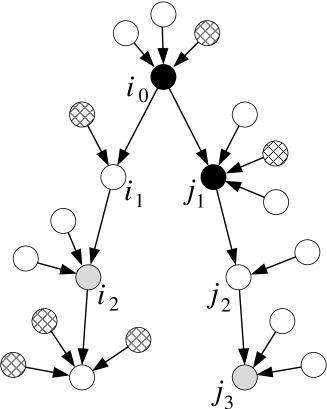
Figure 1: Schematic structure assumed for the mean-field calculation of ${\cal I}_{\infty}$. The average indegree of a node in the network is $K=3$. Black nodes are an example of a directly linked pair. Light grey nodes are an example of a pair that contributes to ${\cal I}_{\infty}$ because of a shared influence ($i_{0}$). Information from $i_{0}$ takes exactly one time step longer (one additional link) to get to the light grey node on the right than to the one on the left. The node labels mark two chains of the type referred to in the text. Hatching indicates frozen nodes.

Now let $\mathbf{P}_{n}$ denote $\mathbf{P}\bm{(}s_{i_{n}}(t),s_{j_{n+1}}(t+1)\bm{)}$ and let

$$\mathbf{B}_{0} \equiv\begin{pmatrix}1-b_{i_{0}}&0\\ 0&b_{i_{0}}\end{pmatrix}\,.$$ (16)

We can then write

$$\mathbf{P}_{n} =\mathbf{T}_{n}\mathbf{T}_{n-1}\cdots\mathbf{T}_{1}\mathbf{B}_{0}(\mathbf{T}^{\prime}_{1})^{\top}(\mathbf{T}^{\prime}_{2})^{\top}\cdots(\mathbf{T}^{\prime}_{n+1})^{\top}\,.$$ (17)

For a given set of the indegrees $k_{i_{1}},\ldots,k_{i_{n}}$ and $k_{j_{1}},\ldots,k_{j_{n+1}}$ denoted by $\mathbf{k}$, we let $\langle I(\mathbf{P}_{n})\rangle_{\mathbf{k}}$ denote the average mutual information associated with $\mathbf{P}_{n}$. Note that $\langle I(\mathbf{P}_{n})\rangle_{\mathbf{k}}$ is the contribution to ${\cal I}_{\infty}$ arising from the average over $i_{n}j_{n+1}$ pair of nodes in chains with a given $\mathbf{k}$.

The average number of occurrences of a feed-forward structure with the vector $\mathbf{k}$ is given by $Nw_{\mathbf{k}}$, where

$$w_{\mathbf{k}} =\prod_{m=1}^{2n+1}k_{m}P(k=k_{m})$$ (18)

and $P(k=k_{m})$ denotes the probability that a randomly selected rule from the rule distribution $R$ has $k_{m}$ inputs.

Putting together Eqs. (8)–(18), we obtain the expression

$${\cal I}_{\infty} =\sum_{n=0}^{\infty}\sum_{\mathbf{k}\in\mathbb{Z}_{+}^{2n+1}}w_{\mathbf{k}}\langle I(\mathbf{P}_{n})\rangle_{\mathbf{k}}$$ (19)

for rule distributions in the disordered regime.

Numerical evaluation of this expression is cumbersome, but can be streamlined substantially by handling the frozen nodes (local biases $b=0$ and $b=1$) analytically. Removing these nodes from the core of the calculations provides additional insights and yields a version of Eq. (19) that can be sampled more efficiently by Monte-Carlo techniques.

The fraction of unfrozen nodes is given by $u=P(B^{*}\notin{0,1})$ and the distribution of local bias in the set of unfrozen nodes is given by $B^{*}_{\textrm{u}}$, where one sample $b$ of $B^{*}_{\textrm{u}}$ is obtained by sampling $b$ from $B^{*}$ repeatedly until a value of $b$ not equal to 0 or 1 is obtained. Similarly, we define an altered rule distribution $R_{\textrm{u}}$. A sample $r_{\textrm{u}}$ from $R_{\rm u}$ is obtained by sampling $r$ from $R$ and fixing each input to $0$ with probability $P(B^{*}=0)$ and $1$ with probability $P(B^{*}=1)$. New samples $r$ are drawn until one obtains a nonconstant function $r_{\textrm{u}}$ of the $k_{\textrm{u}}$ inputs that are not frozen. (The probability of an unfrozen node having a given value of $k_{\textrm{u}}$ is given below.)

We define $\mathbf{P}_{n}^{\textrm{u}}$ and $w_{\mathbf{k}}^{\textrm{u}}$ by replacing $B^{*}$ and $R$ with $B^{*}_{\textrm{u}}$ and $R_{\textrm{u}}$ in the definitions of $\mathbf{P}_{n}$ and $w_{\mathbf{k}}$, respectively. With these definitions, we rewrite Eq. (19) and get

$${\cal I}_{\infty} =u\sum_{n=0}^{\infty}\sum_{\mathbf{k}\in\mathbb{Z}_{+}^{2n+1}}w_{\mathbf{k}}^{\textrm{u}}\langle I(\mathbf{P}_{n}^{\textrm{u}})\rangle_{\mathbf{k}}\,.$$ (20)

Let $R(K)$ denote the rule distribution for a Poissonian distribution of indegrees $k$ such that $\langle k\rangle=K$ and uniform distributions among all Boolean rules with a given $k$. Note that the definition does not require that a rule does depend on all of its inputs. From this point, we restrict the discussion to distributions of the form $R(K)$. We expect the qualitative behavior of this rule distribution to be representative for a broad range of rule distributions. The critical point for $R(K)$ occurs at $K=2$, with ordered networks arising for $K<2$ and disordered networks for $K>2$.

The symmetric treatment of 0s and 1s in the rule distribution simplifies the calculation of $u$ in the sense that it is sufficient to keep track of the probability to obtain constant nodes from $B_{t}$ and there is no need to distinguish nodes that are constantly 1 from those that are constantly 0. Let $u_{t}$ denote $P(B_{t}\notin\{0,1\})$. Then, $u_{t+1}$ can be calculated from $u_{t}$ according to

$$u_{t+1} =e^{-Ku_{t}}\sum_{k=0}\frac{(Ku_{t})^{k}}{k!}\bigl{(}1-2^{2^{k}-1}\bigr{)}\,.$$ (21)

The desired value $u$ is given by the stable fixed point of the map $u_{t}\mapsto u_{t+1}$. Note that this map is identical to the damage control function presented in Ref. Samuelsson and Socolar (2006), meaning that the above determination of $u$ is consistent with the process of recursively identifying frozen nodes without the use of any mean-field assumption.

The rule distribution $R_{\textrm{u}}(K)$ within the set of unfrozen nodes gives a rule with $k_{m}$ inputs with probability

$$P(k_{\textrm{u}}=k_{m}) =e^{-Ku}\frac{(Ku)^{k_{m}}}{u\,k_{m}!}\bigl{(}1-2^{2^{k_{m}}-1}\bigr{)}$$ (22)

The distribution of rules with $k$ inputs is uniform among all nonconstant Boolean rules with the given number of inputs. This expression can be used in Eq. (18). Further analysis is helpful in determining the limiting value of ${\cal I}_{\infty}$ as $K$ approaches its critical value of 2 from above. Appendix A addresses this issue.

II.4 Numerical sampling

We are now in a position to evaluate Eq. (20) by an efficient Monte-Carlo technique. To obtain a distribution that is a good approximation of $B_{\textrm{u}}^{*}$, we use an iterative process to create vectors of samples. Each vector has a fixed number $S$ of samples. The process is initiated by a vector $\mathbf{b}_{0}$ where all $S$ nodes are set to $1/2$. Then a sequence of vectors is created by iteratively choosing a vector $\mathbf{b}_{t+1}$ based on the previous vector $\mathbf{b}_{t}$. To obtain each node in $\mathbf{b}_{t+1}$, we use Eq. (6) with $r$ sampled from $R^{\prime}_{\textrm{u}}(K)$ defined below and $b_{1},\ldots,b_{k}$ being randomly selected elements of $\mathbf{b}_{t}$.

If the rule distribution $R^{\prime}_{\textrm{u}}(K)$ were set to $R_{\textrm{u}}(K)$, the sequence of vectors would fail to converge properly for $K$ that are just slightly larger than $2$. For such $K$, $R_{\textrm{u}}(K)$ gives a 1-input rule with a probability close to 1. This leads to slow convergence and to a proliferation of copies of identical bias values in the sequence of vectors $\{\mathbf{b}_{t}\}$. The remedy for this problem is quite simple. Due to the symmetry between 0 and 1 in the rule distribution, application of a 1-input rule to an input bias distribution $B^{*}$ gives the same output bias distribution $B^{*}$. Thus, we can remove the 1-input rules from $R_{\textrm{u}}(K)$ without altering the limiting distribution at large $t$. We let $R^{\prime}_{\textrm{u}}(K)$ denote the rule distribution obtained by disregarding all 1-input samples from $R_{\textrm{u}}(K)$.

Based on $\{\mathbf{b}_{t}\}$, we construct matrices that can be used for estimating the sums in Eqs. (20) and (48) by random sampling. After an initial number of steps required for convergence, we sample $S$ matrices of the form $\mathbf{P}\bm{(}r(\bm{\sigma})\mid\sigma_{1}\bm{)}$ where $r$ is drawn from $R^{\prime}_{\textrm{u}}(K)$ and the inputs $\sigma_{2},\ldots,\sigma_{k}$ have biases drawn from $\mathbf{b}_{t}$. These matrices and the indegrees of the corresponding rules are stored in the vectors $\mathbf{p}_{t}$ and $\mathbf{k}_{t}$, respectively. The elements of the vectors $\mathbf{b}_{t}$, $\mathbf{p}_{t}$, and $\mathbf{k}_{t}$ are indexed by $i=1,\ldots,S$ and the $i$th element of each vector is denoted by $b_{t,i}$, $\mathbf{p}_{t,i}$, and $k_{t,i}$, respectively. For notational convenience, we define

$$\mathbf{p}_{t,0} =\begin{pmatrix}1&0\\ 0&1\end{pmatrix}\quad{\rm and}\quad k_{t,0}=1$$ (23)

for all $t=0,1,2,\ldots$. With these definitions, the $i=0$ elements correspond to a copy operator.

To estimate the sum in Eq. (20), we truncate it at $n=n_{\textrm{max}}$ where $n_{\textrm{max}}$ is chosen to be sufficiently large for the remaining terms to be negligible. Then we obtain random samples in the following way. We select $i_{0}$ uniformly from $\{1,\ldots,S\}$ and set each of the indices $i_{1},\ldots,i_{n_{\textrm{max}}},j_{1},\ldots,i_{n_{\textrm{max}}+1}$ to $0$ with probability $P(k_{\textrm{u}}=1)$ or to a uniformly chosen sample of $\{1,\ldots,S\}$ with probability $P(k_{\textrm{u}}>1)$. Then we set

$$\mathbf{P}^{\textrm{u}}_{0}=\begin{pmatrix}1-b_{i_{0}}&0\\ 0&b_{i_{0}}\end{pmatrix}(\mathbf{p}_{t,j_{1}})^{\top}\,,\quad\kappa_{0}=k_{t,j_{1}}\,;$$ (24)

and

$$\left.\begin{array}[]{l}\mathbf{P}^{\textrm{u}}_{n}=\mathbf{p}_{t,i_{n}}\mathbf{P}^{\textrm{u}}_{n-1}(\mathbf{p}_{t,j_{n+1}})^{\top}\\ \kappa_{n}=k_{t,i_{n}}\kappa_{n-1}k_{t,j_{n+1}}\end{array}\right\}\textrm{for }n=1,\ldots,n_{\textrm{max}}.$$ (27)

With $I(\mathbf{P}^{\textrm{u}}_{n})$ given by Eq. (15), we construct samples of the mutual information associated with sets of nodes in chain structures:

$$I_{\textrm{chain}} =\sum_{n=0}^{n_{\textrm{max}}}\kappa_{n}I(\mathbf{P}^{\textrm{u}}_{n})\,.$$ (28)

The average value of $I_{\textrm{chain}}$ provides an approximation of the sum in Eq. (20) and we get

$${\cal I}_{\infty} \approx u\langle I_{\textrm{chain}}\rangle\,.$$ (29)

This approximation is good if $t$, $n_{\textrm{max}}$, and $S$ are sufficiently large. For evaluating $\langle I_{\textrm{chain}}\rangle$, we draw $S$ samples of $I_{\textrm{chain}}$ for several subsequent $t$ that are large enough to ensure convergence in $\mathbf{b}_{t}$.

The technique just described is easily generalized to account for uncorrelated noise in the dynamics. To model a system in which each node has a probability $\epsilon$ of generating the wrong output at each time step, we need only modify $r(\bm{\sigma})$ in Eq. (6) and $\mathbf{P}(\beta\mid\alpha)$ of Eq. (8) as follows:

$$r_{\epsilon}(\bm{\sigma}) =(1-\epsilon)\,r(\bm{\sigma})+\epsilon\,[1-r(\bm{\sigma})]$$ (30)

and

$$\mathbf{P}_{\epsilon}(\beta\mid\alpha) =\begin{pmatrix}1-\epsilon&\epsilon\\ \epsilon&1-\epsilon\end{pmatrix}\mathbf{P}(\beta\mid\alpha)\,,$$ (31)

where $\mathbf{P}$ is determined as above by the Boolean rule at a given node. For nonzero $\epsilon$, all nodes are unfrozen, but the calculations proceed exactly as above with $b^{\prime}$ and $\mathbf{P}$ replaced by $b^{\prime}_{\epsilon}$ and $\mathbf{P}_{\epsilon}$, respectively.

We use a similar technique to estimate $\lim_{K\rightarrow 2_{+}}$ based on Eq. (48). The main differences in this technique are that 1-input nodes do not enter the numerical sampling and the sum to be evaluated is two-dimensional rather than one-dimensional.

III Results

III.1 The large system limit

Using the the expressions derived in Section II.3 and the stochastic evaluation techniques described in Section II.4, we have obtained estimates of ${\cal I}_{\infty}$ for $K>2$. Using the expressions in Appendix A, we obtain $\lim_{K\rightarrow 2_{+}}{\cal I}_{\infty}$. The results are shown in Fig. 2.

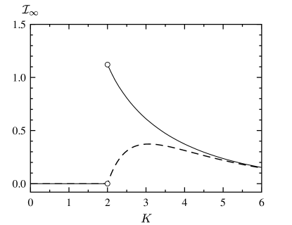
Figure 2: The large system limit ${\cal I}_{\infty}$ for $N\langle I\rangle$ (solid line) and the contribution to ${\cal I}_{\infty}$ from direct information transfer through single nodes (dashed line). The empty circles at the discontinuity of ${\cal I}_{\infty}$ indicate that we do not know the value of ${\cal I}_{\infty}$ for $K=2$. The size of the sample vectors is $S=10^{4}$. The number of vectors used was $10^{3}$–$10^{4}$ and these were drawn after $10^{3}$ steps taken for convergence in $\mathbf{b}_{t}$. The summation cutoff $n_{\textrm{max}}$ varies from $6$ for high $K$ to $100$ for $K$ close to 2. For the limit of ${\cal I}_{\infty}$ for $K\rightarrow 2_{+}$ using Eq. (48), increasing the summation cutoff from $n_{\textrm{max}}=20$ to $n_{\textrm{max}}=40$ gave no significant difference in the result.

The solid line in Fig. 2 shows the full result for ${\cal I}_{\infty}$. The dashed line shows the contribution to ${\cal I}_{\infty}$ that comes from pairs of nodes that are directly linked in the network. It is interesting to note that the direct links alone are not responsible for the peak at criticality. Rather, it is the correlations between indirectly linked nodes that produce the effect, and in fact dominate ${\cal I}_{\infty}$ for $K$ at and slightly above the critical value.

The distribution of local biases plays an important role in determining ${\cal I}_{\infty}$. Biases that are significantly different from $b=1/2$ are important for $K$ that are not deep into the disordered regime, and the distribution of local biases is highly nonuniform. Dense histograms of biases drawn from the distribution $B^{*}_{\textrm{u}}$ for various $K$ are shown in Fig. 3. Singularities at $b=0$ and $b=1$ occur for $K$ in the range $2<K\lesssim 3.4$, and for all $K>2$ there is a singularity at $b=1/2$.

Figure 3: Histograms $h(B^{*}_{\textrm{u}})$ of the distributions of unfrozen local biases $b$ drawn from $B^{*}_{\textrm{u}}$ for $K\rightarrow 2_{+}$ (bold line), $K=3$ (medium line), and $K=4$ (thin line). Bins of width $10^{-4}$ were used to estimate the probability density from a sequence of $10^{6}$ sample vectors $\mathbf{b}_{t}$ that were drawn after $10^{3}$ steps for convergence. The size of the sample vectors is $S=10^{4}$. The combination of a small bin-width and a large sample size enables a clear picture of the strongest singularities.

When uncorrelated noise is added to each node at each time step, ${\cal I}_{\infty}$ may decrease due to the random errors, but may also increase due to the unfreezing of nodes. The net effect as a function of $K$ is shown in Fig. 4 for the case where each output is inverted with probability $\epsilon$ on each time step. As $\epsilon$ is increased from zero, the peak shifts to the disordered regime and broadens. The mutual information due to random unfreezing is clearly visible on the ordered side. In the regime where indirect contributions dominate ${\cal I}_{\infty}$, however, there is a strong decrease as correlations can no longer be maintained over long chains. Deep in the disordered regime, we see the slight decrease expected due to the added randomness. For $\epsilon\gtrsim 0.1$, the maximum of ${\cal I}_{\infty}$ shifts back toward $K=2$. In fact, it can be shown that as $\epsilon$ approaches $1/2$, which corresponds to completely random updating, the ${\cal I}_{\infty}$ curve approaches

$${\cal I}_{\infty}=\frac{K}{\ln 2}\,\biggl{(}\frac{1}{2}-\epsilon\biggr{)}^{\!2}\exp(-K/2)\,.$$ (32)

In this limit, the maximum occurs at $K=2$ and the peak height scales like $(1/2-\epsilon)^{2}$. The fact that the critical $K$ is recovered in the strong noise limit is coincidental; it would not occur for most other choices of Boolean rule distributions.

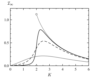
Figure 4: The large system limit ${\cal I}_{\infty}$ as a function of $K$ for various noise levels $\epsilon$ in the updating. The thin solid line shows ${\cal I}_{\infty}$ for networks without noise as displayed in Fig. 2. The other lines represent $\epsilon=0.001$ (thick solid line), $0.01$ (dashed line), and $0.1$ (dotted line). The size of the sample vectors is $S=10^{4}$. $10^{3}$–$10^{6}$ were drawn after $10^{3}$ steps taken for convergence in $\mathbf{b}_{t}$. Extensive sampling was required close to criticality for $\epsilon=0.001$.

III.2 Finite size effects

Numerical simulations on finite networks reveal an important feature near the critical value of $K$ that is not analytically accessible using the above techniques because of the difficulty of calculating ${\cal I}_{\infty}$ right at the critical point. (We have only computed the limit as $K$ approaches $K_{\textrm{c}}$, not the actual value at $K_{\textrm{c}}$.) We compute $\langle I\rangle$ by sampling the mutual information from pairs of nodes from many networks.

In collecting numerical results to compare to the ${\cal I}_{\infty}$ calculation, there are some subtleties to consider. The calculations are based on correlations that persist at long times in the mean-field model. To observe these, one must disregard transient dynamics and also average over the dynamics of different attractors of each network. The latter average should be done by including data from all the attractors in the calculation of the mutual information, not by calculating separate mutual information calculated for individual attractors. For the results presented here, we have observed satisfactory convergence both for increasing lengths of discarded transients and for increasing numbers of initial conditions per network. Finally, an accurate measurement of the mutual information requires sufficiently long observation times; short observation times lead to systematic overestimates of the mutual information. (See, for example, Ref. Bazsó et al. (2004).) In the figures below, the size of the spurious contribution due to finite observation times is smaller than the symbols on the graph.

Fig. 5 shows that the peak in ${\cal I}_{N}$ extends well above the computed ${\cal I}_{\infty}$ value. The figure shows ${\cal I}_{N}$ as a function of $K$ for several system sizes $N$. As $N$ increases, the curve converges toward the infinite $N$ value both in the ordered and disordered regimes. In the vicinity of the critical point, however, the situation is more complicated. The limiting value at criticality will likely depend on the order in which the large size and $K\rightarrow K_{\textrm{c}}$ limits are taken.

We have also studied ${\cal I}_{N}$ as a function of the bias parameter $p$, while holding $K$ fixed at $4$. Fig. 6 shows that ${\cal I}_{N}$ is again peaked at the critical point $p=(2-\sqrt{2})/4$; the qualitative structure of the curves is the same as that for varying $K$. The calculation of ${\cal I}_{\infty}$ for $p\neq 1/2$ requires modifications of the analysis described above that are beyond the scope of this work.

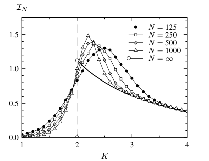
Figure 5: ${\cal I}_{N}$ as a function of $K$ for several different system sizes. For these calculation we use $10^{4}$ networks with $40$ runs from different initial states per network and a discarded transient of length $10^{4}$ updates for each run. (For large $K$, good convergence was obtained for discarded transients of length $10^{3}$.) The sequences of states were recorded for a sample of $10N$ pairs of nodes in each network. The vertical dashed line indicates the critical value of $K$.

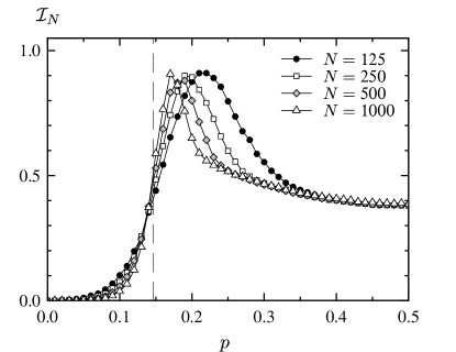
Figure 6: ${\cal I}_{N}$ as a function of $p$ for several different system sizes. For these calculation we use $10^{4}$ networks with $40$ runs from different initial states per network and a discarded transient of length $10^{4}$. (For some data points far into the disordered regime, good convergence was obtained for discarded transients of length $10^{3}$.) The sequences of states were recorded for a sample of $10N$ pairs of nodes in each network. The vertical dashed line indicates the critical value of $p$.

IV Special rule distributions

Up to now, the discussion has focused on rule distributions parametrized only by an independent probability $p$ of finding a $1$ in a given row of the truth table for any given node. Consideration of other possibilities shows that ${\cal I}_{\infty}$ can actually be made as large as desired in networks that are as deep as desired in the disordered regime. Let $\lambda$ be the average sensitivity of a node to its inputs; i.e., the average number of nodes that change values when the value of one randomly selected node is flipped. $\lambda=1$ is one criterion for identifying critical networks Shmulevich and Kauffman (2004). For any value of $\lambda$ in the disordered regime ($\lambda>1$) and any target value ${\cal I}$ of ${\cal I}_{\infty}$, one can always define a rule distribution that gives a random network characterized by $\lambda$ and ${\cal I}$. The key to constructing the distribution is the observation that long chains of single-input nodes produce large ${\cal I}_{\infty}$ and that a small fraction of nodes with many inputs and maximally sensitive rules (multi-input versions of xor) is enough to make $\lambda$ large.

Consider the following class of random networks. Each node has an indegree $k$ of either $1$ or $g$, with the probability of having $g$ inputs being $\gamma$. The logic function at each node is the parity function or its negation. For $k=1$ nodes this means they either copy or invert their input. (There are no nodes with constant outputs.) For $k=g$ nodes it means that a change in any single input causes a change in the output. Note that there are no frozen nodes in these networks.

For these networks, we have

$$\lambda=\langle k\rangle=1-\gamma+g\gamma.$$ (33)

The network consists of $\gamma N$ nodes with multiple inputs, which can be thought of as the roots of a tree of single-input nodes. If $g^{2}\ll\gamma N$, loops in the graph will be rare enough that they will have little effect on the average pairwise mutual information. If $g$ and $\gamma$ are fixed and $N$ is taken to infinity, loops can be neglected in computing ${\cal I}_{\infty}$. For a node with $g>1$, the mutual information between any given input node and the output is zero for the rule distribution under consideration. This is because the bias distribution in networks consisting entirely of maximally sensitive nodes is a delta function at $b=1/2$. Thus $\langle I(\mathbf{P}_{n})\rangle_{\mathbf{k}}=0$ for all $\mathbf{k}\neq\{1,1,\ldots,1\}$. For $\mathbf{k}=\{1,1,\ldots,1\}$, Eq. (18) gives $w_{\mathbf{k}}=(1-\gamma)^{2n+1}$ and we get from Eq. (19):

$${\cal I}_{\infty}=\frac{1-\gamma}{\gamma(2-\gamma)}.$$ (34)

By choosing $\gamma\ll 1$ and $g\gg 1/\gamma$ we can make ${\cal I}_{\infty}$ as large as desired while simultaneously making $\lambda$ as large as desired.

Generalization of this construction to networks with a broader distribution of indegrees and/or rules is straightforward. Roughly speaking, high ${\cal I}_{\infty}$ occurs deep in the disordered regime when there is a small fraction of nodes of high indegree and high sensitivity and the remaining nodes are sensitive to exactly one input.

V Conclusions

In the introduction above, we noted early evidence that eukaryotic cells may be dynamically critical. Our calculations indicate that, within the class of RBNs with randomly assigned inputs to each node and typically studied rule distributions, critical networks provide an optimal capacity for coordinating dynamical behaviors. This type of coordination requires the presence of substantial numbers of dynamical (unfrozen) nodes, the linking of those nodes in a manner that allows long-range propagation of information while limiting interference from multiple propagating signals, and a low error rate. To the extent that evolutionary fitness depends on such coordination and RBN models capture essential features of the organization of genetic regulatory networks, critical networks are naturally favored. We conjecture that mutual information is optimized in critical networks for broader classes of networks that include power-law degree distributions and/or additional local structure such as clustering or over-representation of certain small motifs.

A key insight from our study is that the maximization of average pairwise mutual information is achieved in RBNs by allowing long chains of effectively single-input nodes to emerge from the background of frozen nodes and nodes with multiple unfrozen inputs. The correlations induced by these chains are reduced substantially when stochastic effects are included in the update rules, thus destroying the jump discontinuity in ${\cal I}_{\infty}$ at the critical point and shifting the curve toward the dashed one in Fig. 2 obtained from direct linkages only. Though the noise we have modeled here is rather strong, corresponding to a large fluctuation in the expression of a given gene from its nominally determined value, a shift of the maximum into the disordered regime may be expected to occur in other models.

The behavior of the average pairwise mutual information in RBNs with flat rule distributions is nontrivial and somewhat surprising. This is due largely to the fact that the network of unfrozen nodes in nearly critical systems does indeed have long single-input chains. By choosing a rule distribution carefully, however, we can arrange to enhance the effect and produce arbitrarily high values of ${\cal I}_{\infty}$ even deep in the disordered regime. Whether real biological systems have this option is less clear. The interactions between transcription factors and placement of binding sites required to produce logic with high sensitivity to many inputs appear difficult (though not impossible) to realize with real molecules Buchler et al. (2003).

Maximization of pairwise mutual information may be a sensible proxy for maximization of fitness within an ensemble of evolutionarily accessible networks: we suggest that systems based on high-$\langle I\rangle$ networks can orchestrate complex, timed behaviors, possibly allowing robust performance of a wide spectrum of tasks. If so, the maximization of pairwise mutual information within the space of networks accessible via genome evolution may play an important role in natural selection of real genetic networks. We have found that maximization of pairwise mutual information can be achieved deep in the disordered regime by sufficiently nonuniform Boolean rule distributions. However, in the absence of further knowledge, a roughly flat rule distribution remains the simplest choice, and in this case pairwise mutual information is maximized for critical networks. Given the tentative evidence for criticality in real genetic regulatory networks Shmulevich et al. (2005); Rämö et al. (2006); Serra et al. (2004), these results may be biologically important.

Appendix A Approaching criticality

The mean-field calculations in Section II.3 are not applicable to critical networks, but we can investigate the behavior for disordered networks that are close to criticality. In this appendix, we investigate the limit

$$\lim_{K\rightarrow 2_{+}}{\cal I}_{\infty}$$ (35)

for networks with the rule distribution $R(K)$.

Let $K=2+\epsilon$ where $\epsilon$ is a small positive number. The fraction of unfrozen nodes goes to zero as $\epsilon\rightarrow 0$, meaning that it is appropriate to expand Eq. (21) for small $u_{t}$. A second order Taylor expansion yields

$$u_{t+1} \approx\tfrac{1}{2}Ku_{t}-\tfrac{1}{16}K^{2}u_{t}^{2}$$ (36)

and the fixed point $u$ satisfies

$$1 \approx\tfrac{1}{2}K-\tfrac{1}{16}K^{2}u\,,$$ (37)

meaning that

$$u \approx 8\frac{K-2}{K^{2}}\approx 2\epsilon\,.$$ (38)

Approximation of Eq. (22) to the same order gives

$$P(k_{\textrm{u}}=1) \approx 1-\tfrac{7}{2}\epsilon$$ (39)

and

$$P(k_{\textrm{u}}=2) \approx\tfrac{7}{2}\epsilon\,.$$ (40)

The probability to obtain $k_{\textrm{u}}>2$ vanishes to the first order in $\epsilon$. Equation (40) yields that $P(k_{\textrm{u}}=2)\approx\tfrac{7}{4}u$ for small $\epsilon$. However, all rules with $k_{\textrm{u}}=2$ are not proper 2-input rules in the sense that they do not depend on both inputs. Of the 14 nonconstant Boolean 2-input rules, 4 are dependent on only one input and are effectively 1-input rules. Hence, the probability $p_{2}$ for an unfrozen node to have a proper 2-input rule is given by

$$p_{2} \approx\tfrac{5}{4}u\,.$$ (41)

For small $\epsilon$, nodes with single inputs dominate the expression for $\mathbf{P}_{n}$ in (17). A matrix $\mathbf{T}$ corresponding to a one-input rule is either the unity matrix or a permutation matrix that converts 0s to 1s and vice versa in the probability distribution. None of these matrices has any effect on $\langle I(\mathbf{P}_{n})\rangle$ or $\langle I(\mathbf{P}_{n}^{\textrm{u}})\rangle$, because of the symmetry between 0s and 1s in the rule distribution. Hence, we can express $\langle I(\mathbf{P}^{\textrm{u}}_{n})\rangle_{\mathbf{k}}$ on the form

$$\langle I(\mathbf{P}^{\textrm{u}}_{n})\rangle_{\mathbf{k}} =\langle I(\mathbf{P}^{\textrm{u}}_{(n^{\prime}_{0},n^{\prime}_{1})})\rangle_{\mathbf{k}^{\prime}}\,,$$ (42)

where $n^{\prime}_{0}$ and $n^{\prime}_{1}$, respectively, are the numbers of indegrees $k_{i_{1}},\ldots,k_{i_{n}}$ and $k_{j_{1}},\ldots,k_{j_{n+1}}$ that are different from $1$ and $\mathbf{k}^{\prime}$ is corresponding vector of indegrees different from $1$.

In the limit $\epsilon\rightarrow 0_{+}$, we can neglect indegrees larger than $2$. Hence, we introduce $\langle I(\mathbf{P}_{n_{0},n_{1}}^{(2)})\rangle$ to denote the average mutual information of

$$\mathbf{P}^{(2)}_{(n_{0},n_{1})} =\mathbf{T}_{n}\mathbf{T}_{n-1}\cdots\mathbf{T}_{1}\mathbf{B}_{0}(\mathbf{T}^{\prime}_{1})^{\top}(\mathbf{T}^{\prime}_{2})^{\top}\cdots(\mathbf{T}^{\prime}_{n_{1}})^{\top}\,$$ (43)

where $\mathbf{T}_{1},\ldots,\mathbf{T}_{n}$ and $\mathbf{T}^{\prime}_{1},\ldots,\mathbf{T}^{\prime}_{n^{\prime}}$ correspond to randomly selected 2-input rules that do depend on both inputs. Both $\mathbf{B}_{0}$ and the $\mathbf{T}$-matrices are drawn based on the distribution of local biases obtained by proper 2-input rules only, because the symmetry between 0s and 1s ensures that rules with one input do not alter the equilibrium distribution $B_{\textrm{u}}^{*}$.

Then, Eq. (20) can be approximated by

$${\cal I}_{\infty} \approx u\sum_{n=0}^{\infty}\sum_{n_{0}=0}^{n}\sum_{n_{1}=0}^{n+1}\binom{n}{n_{0}}\binom{n+1}{n_{1}}\langle I(\mathbf{P}_{n_{0},n_{1}}^{(2)})\rangle$$

$$\phantom{\approx}\times(2p_{2})^{n_{0}+n_{1}}(1-p_{2})^{2n+1-n_{0}-n_{1}}$$ (44)

for small $\epsilon$. This approximation is exact in the limit $\epsilon\rightarrow 0_{+}$ and reordering of the summation gives

$$\lim_{\epsilon\rightarrow 0_{+}}{\cal I}_{\infty} =\sum_{n_{0},n_{1}\in\mathbb{N}^{2}}W_{(n_{0},n_{1})}\langle I(\mathbf{P}_{n_{0},n_{1}}^{(2)})\rangle\,,$$ (45)

where

$$W_{(n_{0},n_{1})} \equiv\lim_{\epsilon\rightarrow 0_{+}}u\sum_{n=0}^{\infty}\binom{n}{n_{0}}\binom{n+1}{n_{1}}$$

$$\phantom{\approx}\times(2p_{2})^{n_{0}+n_{1}}(1-p_{2})^{2n+1-n_{0}-n_{1}}$$ (46)

$$=\lim_{\epsilon\rightarrow 0_{+}}\frac{u}{2p_{2}}\binom{n_{0}+n_{1}}{n_{0}}\,.$$ (47)

Because $\lim_{\epsilon\rightarrow 0_{+}}u/(2p_{2})=2/5$, we get

$$\lim_{K\rightarrow 2_{+}}{\cal I}_{\infty} =\frac{2}{5}\sum_{n_{0},n_{1}\in\mathbb{N}^{2}}\binom{n_{0}+n_{1}}{n_{0}}\langle I(\mathbf{P}_{n_{0},n_{1}}^{(2)})\rangle\,.$$ (48)

For approaching the critical point from the ordered regime, we know from the discussion in Section I that

$$\lim_{K\rightarrow 2_{-}}{\cal I}_{\infty} =0\,,$$ (49)

meaning that ${\cal I}_{\infty}$ has a discontinuity at $K=2$. From the scaling of the number of unfrozen nodes and the number of relevant nodes, we expect that ${\cal I}_{\infty}$ is well-defined and different from 0 for $K=2$ but we have found no analytical hints about whether this value is larger or smaller than $\lim_{K\rightarrow 2_{+}}{\cal I}_{\infty}$.

Numerical evaluation of the sum in Eq. (48) is carried out in close analogy with the technique described in Section II.4.

References

- Samuelsson and Socolar (2006) B. Samuelsson and J. E. S. Socolar, Phys. Rev. E 74, 036113 (2006).
- Derrida and Pomeau (1986) B. Derrida and Y. Pomeau, Europhys. Lett. 1, 45 (1986).
- Aldana-Gonzalez et al. (2003) M. Aldana-Gonzalez, S. Coppersmith, and L. P. Kadanoff, in Perspectives and Problems in Nonlinear Science, edited by E. Kaplan, J. E. Marsden and K. R. Sreenivasan (Springer, New York, 2003), p. 23.
- Kauffman (1990) S. A. Kauffman, Physica D 42, 135 (1990).
- Stauffer (1994) D. Stauffer, J. Stat. Phys. 74, 1293 (1994).
- Shmulevich et al. (2005) I. Shmulevich, S. A. Kauffman, and M. Aldana, Proc. Natl. Acad. Sci. USA 102, 13439 (2005).
- Rämö et al. (2006) P. Rämö, J. Kesseli, and O. Yli-Harja, J. Theor. Biol. 242, 164 (2006).
- Serra et al. (2004) R. Serra, M. Villani, and A. Semeria, J. Theor. Biol. 227, 149 (2004).
- Ribeiro et al. (2006) A. S. Ribeiro, R. A. Este, J. Lloyd-Price, and S. A. Kauffman, WSEAS Trans. on Systems 5, 2935 (2006).
- Krawitz and Shmulevich (2007) P. Krawitz and I. Shmulevich, Phys. Rev. Lett. 98, 158701 (2007).
- Luque and Ferrera (2000) B. Luque and A. Ferrera, Complex Systems 12, 241 (2000).
- Bertschinger and Natschläger (2004) N. Bertschinger and T. Natschläger, Neural Comput. 16, 1413 (2004).
- Bazsó et al. (2004) F. Bazsó, L. Zalányi, and A. Petróczi, Proc. IEEE Intl. Joint Conf. on Neural Net. 4, 2843 (2004).
- Shmulevich and Kauffman (2004) I. Shmulevich and S. A. Kauffman, Phys. Rev. Lett. 93, 048701 (2004).
- Buchler et al. (2003) N. E. Buchler, U. Gerland, and T. Hwa, Proc. Natl. Acad. Sci. USA 100, 5136 (2003).