$V_{us}$ Calculation from Lattice QCD

Abstract

I review recent progress in calculating $|V_{us}|$ from lattice QCD kaon and hyperon systems. A preliminary result from the first dynamical calculation in the hyperon channel is included.

I Introduction

The Standard Model has successfully described strong interactions using a quantum field theory where universe contains quarks of three generations, which interact via gauge bosons, the gluons. Although electromagnetism and the strong interaction are not affected by quark flavor, the weak interaction may change the flavor of the quarks. This overlap between the various generations is described by the Cabibbo-Kobayashi-Maskawa (CKM) matrix.

In 1963, Cabibbo first introduced a $2\times 2$ quark mixing matrix to explain semileptonic decay in baryons; Kobayashi and Maskawa later extended the matrix to include the then-undiscovered bottom quark sector. This becomes the CKM matrix that we are familiar with today:

$$V_{\rm CKM}=\left(\begin{array}[]{ccc}V_{ud}&V_{us}&V_{ub}\\ V_{cd}&V_{cs}&V_{cb}\\ V_{td}&V_{ts}&V_{tb}\\ \end{array}\right).$$ (4)

The Standard Model requires this matrix to be unitary. This gives six unitarity constraints, each of which may be graphically depicted as a unitarity triangle; one such constraint is

$$|V_{ud}|^{2}+|V_{us}|^{2}+|V_{ub}|^{2}=1.$$ (5)

From the latest PDG 2006Yao et al. (2006), $V_{ud}$ in this unitarity equation is both the dominant term and also very well determined from neutron beta decay, 0.97377(27); $V_{ub}$ is very small, $4.21(30)\times 10^{-3}$. This leaves the middle matrix element $V_{us}$ as the weak link in deciding whether or not this unitarity equation holds. In latest PDG edition, $V_{us}=0.2257(21)$ is determined to only 0.1%. In this proceeding, I will describe how this number can be obtained using calculations from lattice QCD. Note that although currently $V_{us}$ seems to indicate that this unitarity equation holds within error bars, the number has been shifting around a lot during the past few years. In 2003, it was 0.2195(23), which is more than 10 standard deviations away from its current best value.

In quantum chromodynamics (QCD), physical observables are calculated from the path integral. For calculations where the coupling is weak, one can perform the integral by hand. However, for long distances the perturbative QCD series no longer converges. Thus, to calculate from first principles, one needs help from lattice gauge theory. Lattice QCD discretizes space-time such that the path integral over field strengths (especially at strong coupling) can be calculated numerically. Since the real world is continuous and infinitely large, at the end of the day we will have to take the lattice spacing $a\rightarrow 0$ and the volume $V\rightarrow\infty$ limits to connect to the physical world. However, to simulate at the real pion mass (while at the same time keeping the lattice box big enough to avoid finite-volume effects) would require much faster supercomputers that have not yet been born. Thus, we normally calculate with a few unrealistically large values of the pion mass and then use chiral extrapolation to get back to the physical pion mass.

Here, we quickly mention a few choices of fermion action that have been commonly used in lattice QCD calculations. Each has its own pros and cons. They differ primarily by how they maintain symmetry, their calculation cost and their discretization error. (Improved) Staggered fermions (asqtad)Kogut and Susskind (1975); Orginos and Toussaint (1999); Orginos et al. (1999) are relatively cheap for dynamical fermions, but they introduce mixing among parities and flavors or “tastes”, which make baryonic operators a nightmare to deal with. The $O(a)$-improved Wilson (clover) fermion actionSheikholeslami and Wohlert (1985) is moderate in cost and free of the disadvantages of the staggered actions. However, chiral symmetry is badly broken at non-zero lattice spacing which causes operator mixing issues. Chiral fermions (e.g. domain-wall (DWF) or overlap)Kaplan (1992, 1993); Shamir (1993); Furman and Shamir (1995) are free of all the above problems. They are automatically $O(a)$ improved, suitable for spin physics and weak matrix elements. These benefits come at great computational cost. Last but not least are mixed actions, where one chooses difference valence and sea quark discretizations. Later in this work, we present work done using staggered sea quarks (cheap) with domain-wall valence quarks (chiral); we match the sea Goldstone pion mass to the DWF pion.

Before we discuss the details of the lattice calculation, it is important to mention the “quenched” approximation or 0-flavor calculations. There are a couple of calculations mentioned later which use this approximation. In the path integral, the correct way to carry out the fermionic part of integral is to integrate out the quark/antiquark fields first. This leaves the remaining integral as a function only of the gauge links and introduces a fermionic determinant. The “quenched” approximation fixes the fermionic determinant as a constant. This means that when we calculate, say, a two-point Green function, as depicted in Figure 1, such as a meson correlator, internal fermion loops have been omitted.

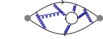
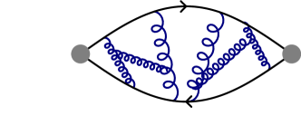
Figure 1: A depiction of the difference between full QCD and the quenched approximation in the example of a two-point Green function.

The quenched approximation was a product of the old days when computers were slow and algorithms were not yet sped up to today’s standards. Quenching very greatly reduces the cost of a lattice calculation by eliminating the fermionic determinant. Of course, modern calculations have moved on to focus on unquenched calculations. This is a lot better, since when one ignores the fermion loops, it is very difficult to estimate how much this will affect the final numbers; the size of the effect tends to vary greatly between different physical quantities. However, since calculations using the quenched approximation can be done very fast, one can test new methodologies and ideas using this approximation before performing unquenched (dynamical) calculations. The first lattice calculations in $K_{l3}$ and hyperon semileptonic decay were demonstrated in this approximation.

In the following, I will review the latest $V_{us}$ calculations. There has been a series of works devoted to $K_{l3}$ decays but only quenched calculations in the hyperon channel so far. In the second half of this work, I will show the first lattice dynamical calculation of hyperon decays using mixed action. In the final part, I will summarize the current standing of $V_{us}$ from lattice QCD and give some future outlook.

II Lattice $V_{us}$ Calculations

In this work, we will concentrate on three determinations of $V_{us}$: leptonic decay ratios (mainly for completion), $K_{l3}$ decays and hyperon decays. We will compare all of them to the number listed in PDG 2006. So far, the number from $K_{l3}$ decays has the smallest errorbar for $V_{us}$.

II.1 Leptonic Decays

If one looks at the decays $K_{\mu 2}$ and $\pi_{\mu 2}$, their branching ratios can be written in terms of $V_{us}/V_{ud}$ and the ratio of the kaon to pion decay constant:

$$\left(\frac{\left|V_{us}\right|}{\left|V_{ud}\right|}\right)^{2}=\left[\left(\frac{f_{K}}{f_{\pi}}\right)^{2}\frac{M_{K}\left(1-m_{\mu}^{2}/M_{K}^{2}\right)^{2}}{M_{\pi}\left(1-m_{\mu}^{2}/M_{\pi}^{2}\right)^{2}}\left(1+\frac{\alpha}{\pi}\left(C_{K}-C_{\pi}\right)\right)\right]^{-1}\frac{\Gamma(K\rightarrow\mu\bar{\nu}_{\mu})}{\Gamma(\pi\rightarrow\mu\bar{\nu}_{\mu})},$$ (6)

where $C_{K}$ and $C_{\pi}$ are the radiative-inclusive electroweak corrections, and the rest of the numbers can be obtained from experimental measurements. W. J. MarcianoMarciano (2004) used decay constant ratios $f_{K}/f_{\pi}=1.210(4)(13)$ from a 2+1f staggered fermion calculation of $f_{\pi}$ and $f_{K}$ done in 2004 by MILC collaboration and found $V_{us}=0.2219(25)$. Of course, there have been other full-QCD calculations since 2004. For example, RBC/UKQCD use dynamical chiral fermions (DWF) to obtain the ratio 1.24(2)Allton et al. (2007). However, none of the other collaborations have come out with a number with competitive errorbar yet. In 2006, MILC updated their own calculation, $1.208(2)(^{7}_{14})$Bernard et al. (2006); this yields $V_{us}=0.2223(^{26}_{14})$.

II.2 $K_{l3}$ Decay

Another way to determine $V_{us}$ is to look at the $K_{l3}$ decay. When one integrates out the short-distance dependence, one is left with a low-energy non-perturbative matrix element for K to $\pi$, which can be calculated directly in lattice QCD. Using Lorentz invariance, we can decompose the matrix element into two form factors ($f_{+}$ and $f_{-}$) with differing momentum dependence:

$$\langle\pi(p^{\prime})|V_{\mu}|K(p)\rangle=(p_{\mu}+p^{\prime}_{\mu})f_{+}(q^{2})+(p_{\mu}-p^{\prime}_{\mu})f_{-}(q^{2}).$$ (7)

The so-called “double ratio” technique:

$$\frac{\langle\pi|\overline{s}\gamma_{0}u|K\rangle\langle K|\overline{u}\gamma_{0}s|\pi\rangle}{\langle K|\overline{s}\gamma_{0}s|K\rangle\langle\pi|\overline{u}\gamma_{0}u|\pi\rangle}=|f_{0}(q_{\rm max}^{2})|^{2}\frac{(m_{K}+m_{\pi})^{2}}{4m_{K}m_{\pi}},$$ (8)

which has been used to look at $B$-to-$D$ decaysHashimoto et al. (2000), can also be applied to the $K$ to $\pi$ decay. The result is a form factor that only depends on $q^{2}$, the momentum transfer between the initial and final states, and some kinetic factors. This $f_{0}$ can be connected to $f_{\pm}$ through

$$f_{0}(q^{2})=f_{+}(q^{2})+\frac{q^{2}}{m_{K}^{2}-m_{\pi}^{2}}f_{-}(q^{2}).$$ (9)

When we extrapolate to $q^{2}=0$, $f_{0}=f_{+}$. We study different extrapolation forms to estimate the systematic error caused by our extrapolation:

$$f_{0}(q^{2})^{\rm Linear} = f_{0}(0)(1+\lambda_{0}q^{2})$$ (10)

$$f_{0}(q^{2})^{\rm Quadratic} = f_{0}(0)(1+\lambda_{0}q^{2}+cq^{4})$$ (11)

$$f_{0}(q^{2})^{\rm Polar} = f_{0}(0)/(1-\lambda_{0}q^{2}),$$ (12)

which are shown in Figure 2 by Becirevic et al.Becirevic et al. (2005a).

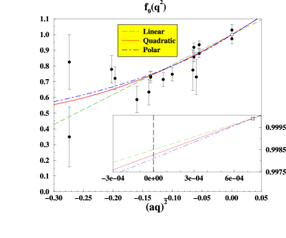
Figure 2: Momentum extrapolation from Ref. Becirevic et al. (2005a)

To remove uncertainty due to the momentum extrapolation, we can calculate the matrix element directly at $q^{2}=0$. The trick to this technique is to include help from “twisted” boundary conditions on the fermions as

$$\psi(x+e_{j}L)=e^{2\pi i\theta_{j}}\psi(x).$$ (13)

The discretized momenta on the lattice will reflect the choice of this $\theta_{j}$ as $p_{j}=\theta_{j}\frac{2\pi}{L}+n_{j}\frac{2\pi}{L}$ with $n_{j}$ integer. We can select $\theta$ wisely to cancel out the mass difference, so that we can obtain $f_{+}(0)$ directly. Guadagnoli et al.Guadagnoli et al. (2006) first demonstrated the advantage in the quenched approximation. Later, UKQCD made an exploratory study on a 2+1-flavor DWF calculationBoyle et al. (2007). They showed that with 50% more statistics, one can get number competitive with conventional extrapolation calculations. The advantage of this method over the conventional one is smaller or no systematic error due to $q^{2}$ extrapolation. Thus, total error on the calculation is reduced.

After we obtain $f_{0}(0)$, the next step is to extrapolate the pion mass to the physical one. We can get some help from the Ademollo-Gatto (AG) theoremAdemollo and Gatto (1964); Becirevic et al. (2006). We know that the $SU(3)$ symmetry-breaking Hamiltonian is

$$H=\frac{1}{\sqrt{3}}\left(m_{s}-\frac{m_{d}+m_{u}}{2}\right)\overline{q}\lambda^{8}q.$$ (14)

The AG theorem tells us that there is no first-order correction due to $SU(3)$-breaking; thus, the correction starts at second order

$$f_{0}(0)=f_{0}(0)^{SU(3)}+O(H^{2}).$$ (15)

What would be a good measure for $SU(3)$ breaking? The most natural candidate would be the mass splitting between the kaon and pion. So, we expect the remaining correction should be small; thus, one would expect the “corrected” lattice $f_{0}$ (after subtracting the chiral log), $f^{\prime}$, should differ from $f_{0}^{SU(3)}$ by only a small amount. We construct a ratio

$$R(m_{K},m_{\pi})=\frac{f^{SU(3)}-|f^{\prime}(0)|}{a^{4}(m_{K}^{2}-m_{\pi}^{2})^{2}},$$ (16)

where $f^{SU(3)}$ is the $SU(3)$-limit value; in this case, it is 1. We expect the remaining mass dependence in Eq. 16 should be relatively small. We then extrapolate the remaining mass dependence to the physical sum of the pion and kaon masses-square

$$R(m_{K},m_{\pi})=c_{0}+c_{1}{a^{2}(m_{K}^{2}+m_{\pi}^{2})}.$$ (17)

Thus, $V_{us}$ can then be obtained from

$$\Gamma(K_{l3})=\frac{G_{F}^{2}M_{K}^{5}}{128\pi^{3}}|V_{us}|^{2}S_{\rm EW}|f_{+}(0)|^{2}C_{K}^{2}I_{K}^{l}(\lambda_{i})(1+\delta_{SU(2)}^{K}+\delta_{\rm EM}^{K}).$$ (18)

The decay width, $\Gamma(K_{l3})$, is taken from experiment, while the phase-space integral $I_{K}^{l}$, isospin breaking $\delta_{SU(2)}^{K}$, long-distance electromagnetic corrections $\delta_{\rm EM}^{K}$ and short-distance radiative corrections $S_{\rm EW}$ are taken from perturbative calculations.

Table 1 summarizes the results from various lattice QCD groups: quenched, partially quenched and full QCD, fermion action variety and the range of the pion mass. Figure 3 $f_{+}$ is taken from individual calculations, combined with the latest PDG 2006 number for $|f_{+}V_{us}|=0.2169(9)$. Note the $V_{us}$ number may be different from the ones given in the original papers, due to progress in experimental measurements. The grey band in the graph is the range allowed assuming unitarity holds. All the lattice calculations so far have agreed with the old estimation from Leutwyler-Roos in 1984Leutwyler and Roos (1984). However, not every paper has complete estimations of the systematic errors due to lattice artifacts. The work done by RBC/UKQCDAntonio et al. (2007) is one of the exceptions, and thus I quote their number as representative of the $V_{us}$ from $K_{l3}$ decay channel: 0.2257(14).

Group	$N_{\rm f}$	$S_{\rm f}$	$M_{\pi}$ (GeV)	# conf	$f_{+}(0)$
SPQcdRBecirevic et al. (2005b)	0	Wilson	0.500–1.000	230	0.961(09)
JLQCDTsutsui et al. (2006)	2	Clover	0.440–$0.960^{*}$	N/A	0.967(06)
RBCDawson et al. (2006)	2	DWF	0.475–0.700	94	0.955(12)
HPQCDOkamoto (2006)	2+1	Staggered	0.500–0.700	N/A	0.962(11)
RBC/UKQCDAntonio et al. (2007)	2+1	DWF	0.390–0.700	150	0.961(05)

Table 1: Summary of existing published $f_{+}$ calculations from $K_{l3}$ decay

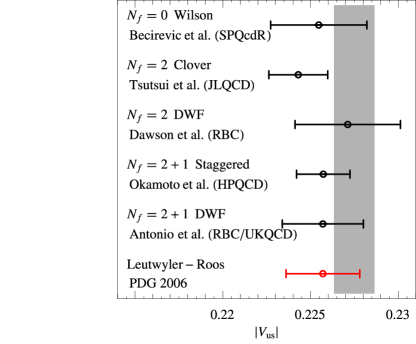
Figure 3: Lattice $|V_{us}|$ summary with unified experimental numbers from PDG

II.3 Hyperon Decays

Hyperon decays provide us with an additional independent channel for determining $V_{us}$. We start by looking at the low-energy contribution of the transition matrix elements for hyperon beta decay, $B_{1}\rightarrow B_{2}e^{-}\overline{\nu}$; in low-energy effective theory this can be written as

$${\cal M}=\frac{G_{s}}{\sqrt{2}}\overline{u}_{B_{2}}(O_{\alpha}^{\rm V}+O_{\alpha}^{\rm A}){u}_{B_{1}}\overline{u}_{e}\gamma^{\alpha}(1+\gamma_{5})v_{\nu}.$$ (19)

From Lorentz symmetry, we expect the matrix element composed of any two spin-$1/2$ nucleon states, $B_{1}$ and $B_{2}$, to have the general form

$$O_{\alpha}^{V} = f_{1}(q^{2})\gamma^{\alpha}+\frac{f_{2}(q^{2})}{M_{B_{1}}}\sigma_{\alpha\beta}q^{\beta}+\frac{f_{3}(q^{2})}{M_{B_{1}}}q_{\alpha}$$ (20)

$$O_{\alpha}^{A} = \left(g_{1}(q^{2})\gamma^{\alpha}+\frac{g_{2}(q^{2})}{M_{B_{1}}}\sigma_{\alpha\beta}q^{\beta}+\frac{g_{3}(q^{2})}{M_{B_{1}}}q_{\alpha}\right)\gamma_{5}$$ (21)

with transfer momentum $q=p_{B_{2}}-p_{B_{1}}$ and $V,A$ indicating the vector and axial currents respectively.

The vector form factor is connected to $V_{us}$ via

$$\Gamma = G_{F}^{2}\,|V_{us}|^{2}\,\frac{\Delta m^{5}}{60\pi^{3}}\,(1+\delta_{\rm rad})$$ (23)

$$\!\!\!\!\!\!\times\left[\left(1-\frac{3}{2}\,\beta\right)\left(|f_{1}|^{2}+|g_{1}|^{2}\right)+\frac{6}{7}\,\beta^{2}\left(|f_{1}|^{2}+2|g_{1}|^{2}+\text{Re}(f_{1}f_{2}^{*})+\frac{2}{3}\,|f_{2}^{2}|\right)+\delta_{q^{2}}\right],$$

with $\Delta m=m_{B_{1}}-m_{B_{2}}$, $\beta=\Delta m/m_{B_{1}}$, the radiative corrections $\delta_{\rm rad}$, and $\delta_{q^{2}}(f_{1},g_{1})$ taking into account the transfer-momentum dependence of $f_{1}$ and $g_{1}$ Garcia et al. (1985). Generally, the ratios of $g_{1}/f_{1}$ from experiment and $f_{2}/f_{1}$ in the $SU(3)$ limit are used to get $V_{us}$ from hyperon decays.

In 2003, Cabibbo et al.Cabibbo et al. (2003) used $f_{2}/f_{1}$ and $f_{1}$ in the $SU(3)$ limit, combined with the experimental decay width (or rate) and $g_{1}/f_{1}$, to obtain $V_{us}$ from various channels of hyperon decay, as shown in Table 2. It is not hard to see that if lattice calculations can provide better estimates of $g_{1}/f_{1}$, we can improve the precision of $V_{us}$ from hyperon decays and possibly get a better estimation than the $K_{l3}$ channel.

Channel	$f_{1}^{SU(3)}$	$|f_{1}V_{us}|$	$\left({g_{1}}/{f_{1}}\right)^{SU(3)}$	$\left({g_{1}}/{f_{1}}\right)^{\rm exp}$
$n\rightarrow p$	1	$n/a$	$F+D$	$1.2670(30)$
$\Lambda\rightarrow p$	$-\sqrt{3/2}$	$0.2221(33)$	$F+D/3$	$0.718(15)$
$\Sigma^{-}\rightarrow n$	$-1$	$0.2274(49)$	$F-D$	$-0.340(17)$
$\Xi^{-}\rightarrow\Lambda$	$\sqrt{3/2}$	$0.2367(97)$	$F-D/3$	$0.25(5)$
$\Xi^{-}\rightarrow\Sigma^{0}$	$\sqrt{1/2}$	$n/a$	$F+D$	$n/a$
$\Xi^{0}\rightarrow\Sigma^{+}$	1	$0.216(33)$	$F+D$	$1.32(22)$

Table 2: Summary of a few hyperon numbers

So far, there are only two quenched lattice calculations of hyperon beta decay, and they are in different channels, $\Sigma\rightarrow n$ and $\Xi^{0}\rightarrow\Sigma^{+}$. Guadagnoli et al.Guadagnoli et al. (2007) extrapolate the matrix element $\Sigma\rightarrow n$ via an AG ratio, similar to the discussion in the $K_{l3}$ decay case, but using a dipole form to extrapolate to the zero-transfer momentum point. All of the pion masses are larger than 700 MeV; their final numbers are $f_{1}=-0.988(29)_{\rm stat}$ and $V_{us}=0.230(5)_{\rm exp}(7)_{\rm lat}$. Sasaki et al.Sasaki and Yamazaki (2006) use lighter pion masses 530–650 MeV and DWF to look at the $\Xi^{0}$ decay channel. They extrapolate the vector form factor $f_{1}$ via the variable $\delta=(m_{B_{2}}-m_{B_{1}})/m_{B_{2}}$. The Ademollo-Gatto theorem suggests the leading-order effect should be $\delta^{2}$, and thus one can fit $f_{1}(0)$ to the form $c_{0}+c_{1}\delta^{2}$. Their final numbers are $f_{1}=0.953(24)_{\rm stat}$ and $V_{us}=0.219(27)_{\rm exp}(5)_{\rm lat}$. Unfortunately, the experimental determination of the decay rate is lousy; despite $f_{1}$ in $\Xi$ decay channel being compatible within errors, $V_{us}$ is not well-determined. This may further improve in the future with updates from Fermilab KTeV and CERN NA48 collaborations. One important thing to note is that neither of the calculations has systematic error estimates from quenching effects, which we expect might be significant.

We have taken data looking at both hyperon channels with a dynamical lattice calculation for the first time. We use a mixed action, meaning that the sea (staggered) and valence (DWF) fermions have different discretization. Our pion masses are relatively lighter than the quenched calculations. We only simulate one strange quark mass, which unfortunately does not reproduce the correct strange-strange Goldstone mesons. We find a box size around 2.6 fm and list a few other important parameters in Table 3. In this work, we report on our preliminary calculation in the $\Sigma^{-}\rightarrow n$ channel. We use a projection operator $T=(1-\gamma_{5}\gamma_{3})(1+\gamma_{4})/2$ in both two- and three-point Green functions and construct a ratio

$$R_{j_{\mu}} = \frac{Z_{V}\Gamma^{\Sigma N}_{\mu,GG}(t_{i},t,t_{f},{\mathchoice{\!\stackrel{{\scriptstyle{}_{{}_{\>\scriptstyle\rightarrow}}}}{{\displaystyle p}}\!}{\!\stackrel{{\scriptstyle{}_{{}_{\>\scriptstyle\rightarrow}}}}{{\textstyle p}}\!}{\!\stackrel{{\scriptstyle{}_{{}_{\>\scriptscriptstyle\rightarrow}}}}{{\scriptstyle p}}\!}{\!\stackrel{{\scriptstyle{}_{{}_{\>\scriptscriptstyle\rightarrow}}}}{{\scriptscriptstyle p}}\!}}_{i},{\mathchoice{\!\stackrel{{\scriptstyle{}_{{}_{\>\scriptstyle\rightarrow}}}}{{\displaystyle p}}\!}{\!\stackrel{{\scriptstyle{}_{{}_{\>\scriptstyle\rightarrow}}}}{{\textstyle p}}\!}{\!\stackrel{{\scriptstyle{}_{{}_{\>\scriptscriptstyle\rightarrow}}}}{{\scriptstyle p}}\!}{\!\stackrel{{\scriptstyle{}_{{}_{\>\scriptscriptstyle\rightarrow}}}}{{\scriptscriptstyle p}}\!}}_{f}\,;\;T)}{\Gamma^{NN}_{GG}(t_{i},t_{f},{\mathchoice{\!\stackrel{{\scriptstyle{}_{{}_{\>\scriptstyle\rightarrow}}}}{{\displaystyle p}}\!}{\!\stackrel{{\scriptstyle{}_{{}_{\>\scriptstyle\rightarrow}}}}{{\textstyle p}}\!}{\!\stackrel{{\scriptstyle{}_{{}_{\>\scriptscriptstyle\rightarrow}}}}{{\scriptstyle p}}\!}{\!\stackrel{{\scriptstyle{}_{{}_{\>\scriptscriptstyle\rightarrow}}}}{{\scriptscriptstyle p}}\!}}_{f}\,;\;T)}\sqrt{\frac{\Gamma^{\Sigma\Sigma}_{PG}(t,t_{f},{\mathchoice{\!\stackrel{{\scriptstyle{}_{{}_{\>\scriptstyle\rightarrow}}}}{{\displaystyle p}}\!}{\!\stackrel{{\scriptstyle{}_{{}_{\>\scriptstyle\rightarrow}}}}{{\textstyle p}}\!}{\!\stackrel{{\scriptstyle{}_{{}_{\>\scriptscriptstyle\rightarrow}}}}{{\scriptstyle p}}\!}{\!\stackrel{{\scriptstyle{}_{{}_{\>\scriptscriptstyle\rightarrow}}}}{{\scriptscriptstyle p}}\!}}_{i}\,;\;T)}{\Gamma^{NN}_{PG}(t,t_{f},{\mathchoice{\!\stackrel{{\scriptstyle{}_{{}_{\>\scriptstyle\rightarrow}}}}{{\displaystyle p}}\!}{\!\stackrel{{\scriptstyle{}_{{}_{\>\scriptstyle\rightarrow}}}}{{\textstyle p}}\!}{\!\stackrel{{\scriptstyle{}_{{}_{\>\scriptscriptstyle\rightarrow}}}}{{\scriptstyle p}}\!}{\!\stackrel{{\scriptstyle{}_{{}_{\>\scriptscriptstyle\rightarrow}}}}{{\scriptscriptstyle p}}\!}}_{f}\,;\;T)}}$$ (24)

$$\times \sqrt{\frac{\Gamma^{NN}_{GG}(t_{i},t,{\mathchoice{\!\stackrel{{\scriptstyle{}_{{}_{\>\scriptstyle\rightarrow}}}}{{\displaystyle p}}\!}{\!\stackrel{{\scriptstyle{}_{{}_{\>\scriptstyle\rightarrow}}}}{{\textstyle p}}\!}{\!\stackrel{{\scriptstyle{}_{{}_{\>\scriptscriptstyle\rightarrow}}}}{{\scriptstyle p}}\!}{\!\stackrel{{\scriptstyle{}_{{}_{\>\scriptscriptstyle\rightarrow}}}}{{\scriptscriptstyle p}}\!}}_{f}\,;\;T)}{\Gamma^{\Sigma\Sigma}_{GG}(t_{i},t,{\mathchoice{\!\stackrel{{\scriptstyle{}_{{}_{\>\scriptstyle\rightarrow}}}}{{\displaystyle p}}\!}{\!\stackrel{{\scriptstyle{}_{{}_{\>\scriptstyle\rightarrow}}}}{{\textstyle p}}\!}{\!\stackrel{{\scriptstyle{}_{{}_{\>\scriptscriptstyle\rightarrow}}}}{{\scriptstyle p}}\!}{\!\stackrel{{\scriptstyle{}_{{}_{\>\scriptscriptstyle\rightarrow}}}}{{\scriptscriptstyle p}}\!}}_{i}\,;\;T)}}\sqrt{\frac{\Gamma^{NN}_{PG}(t_{i},t_{f},{\mathchoice{\!\stackrel{{\scriptstyle{}_{{}_{\>\scriptstyle\rightarrow}}}}{{\displaystyle p}}\!}{\!\stackrel{{\scriptstyle{}_{{}_{\>\scriptstyle\rightarrow}}}}{{\textstyle p}}\!}{\!\stackrel{{\scriptstyle{}_{{}_{\>\scriptscriptstyle\rightarrow}}}}{{\scriptstyle p}}\!}{\!\stackrel{{\scriptstyle{}_{{}_{\>\scriptscriptstyle\rightarrow}}}}{{\scriptscriptstyle p}}\!}}_{f}\,;\;T)}{\Gamma^{\Sigma\Sigma}_{PG}(t_{i},t_{f},{\mathchoice{\!\stackrel{{\scriptstyle{}_{{}_{\>\scriptstyle\rightarrow}}}}{{\displaystyle p}}\!}{\!\stackrel{{\scriptstyle{}_{{}_{\>\scriptstyle\rightarrow}}}}{{\textstyle p}}\!}{\!\stackrel{{\scriptstyle{}_{{}_{\>\scriptscriptstyle\rightarrow}}}}{{\scriptstyle p}}\!}{\!\stackrel{{\scriptstyle{}_{{}_{\>\scriptscriptstyle\rightarrow}}}}{{\scriptscriptstyle p}}\!}}_{i}\,;\;T)}},$$

to cancel out kinetic and overlap $Z$ factors. With multiple insertions of the momentum, we can solve for the individual form factors in Eq. 20.

Label	$m_{\pi}$ (MeV)	$m_{K}$ (MeV)	$\Sigma^{-}\rightarrow n$ conf.
m010	358(2)	605(2)	600
m020	503(2)	653(2)	420
m030	599(1)	688(2)	561
m040	689(2)	730(2)	306

Table 3: Configuration information

We need to extrapolate to zero momentum. We use a dipole form, as has been used in momentum extrapolation for many baryons’ momentum dependence. For the mass extrapolation, a similar approach to the $K_{l3}$ case can be applied here with the help of the Ademollo-Gatto theorem. We first construct a ratio and then extrapolate the mass dependence according to Eq. 16, as shown in Figure 4. Since our heaviest pion mass is much closer to the strange Goldstone meson mass, due to the mass difference in the denominator of the ratio, the magnitudes of this point, both central value and especially the errorbar, increase a lot. Thus, it provides only a very weak constraint to the fit; this is not an ideal solution for our data.

Alternatively, we can combine the given two-step process into one, by performing a two-dimensional fit to the sum and difference of kaon and pion masses, as shown in Figure 5. But this fit is not ideal either since the constraints from the data points are not strong: only four points to define a two-dimensional surface.

A better constrained fit can be composed by combining the momentum and mass dependence into a single simultaneous fit:

$$f_{1}(q^{2})=\frac{1+\left(M_{K}^{2}-M_{\pi}^{2}\right)^{2}\left(A_{1}+A_{2}\left(M_{K}^{2}+M_{\pi}^{2}\right)\right)}{\left(1-\frac{q^{2}}{M_{0}+M_{1}\left(M_{K}^{2}+M_{\pi}^{2}\right)}\right)^{2}}.$$ (25)

Figure 6 shows the result from simultaneously fitting over all $q^{2}$ and mass combinations. The $z$-direction indicates $f_{1}$, while the $x$- and $y$-axes indicate mass and transfer momentum. The surface is the fit using Eq. 25 with color to indicate different masses. The columns are the data and the momentum points from different pion masses line up in bands. Our preliminary result for $f_{1}$ is $-0.88(15)$. This leads us to a $V_{us}$ somewhat larger in central value than the other calculations but still agrees with them due to the large errorbar. The statistics will be greatly improved at the lightest pion mass data in the near future.

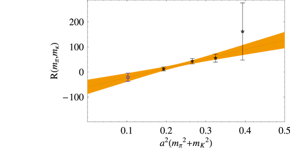
Figure 4: AG ratio extrapolation to physical $m_{K}^{2}+m_{\pi}^{2}$

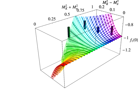
Figure 5: Two-dimensional mass extrapolation after dipole extrapolation to zero-transfer point

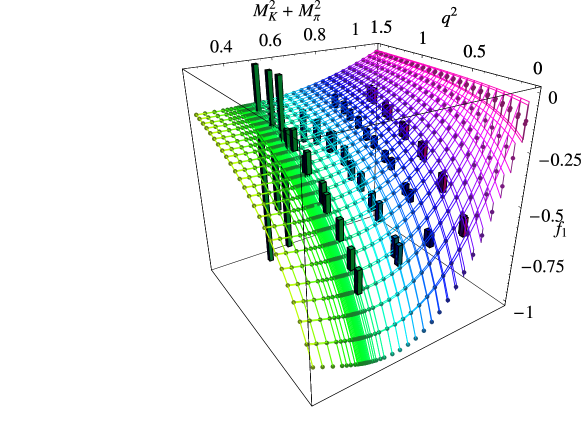
Figure 6: Simultaneous extrapolation in $q^{2}$ and mass

III Conclusion and Outlook

To summarize, there are various ways that lattice QCD calculations can help to determine $V_{us}$ in the CKM matrix. (Similar approaches can be applied to the rest of the elements with effective lattice fermion actions.) Firstly, we can use the lattice input from the kaon and pion decay constant ratios. Currently, MILC has best determined ones, resulting in $V_{us}=0.2226(^{26}_{15})$. Secondly, we can use the form factor from $K_{l3}$ decay matrix elements: here we use the number from RBC/UKQCD, 0.2257(14), in which a sound study and proper systematics are included.

Finally, we can use the form factors from hyperon decays. We have started the first full-QCD 2+1-flavor dynamical calculation. Our preliminary results show consistency with previous calculations, but have larger errorbar due to the choice of lighter pion mass. The larger statistical error is partially compensated by the decrease in systematic error due to extrapolating the pion mass to the physical one. To improve the $V_{us}$ value from the hyperon decays, we need to reduce our statistical error on the vector form factor and improve the accuracy on $g_{1}/f_{1}$ to replace the experimental one. Using these strategies, we can make our calculation of $|V_{us}|$ equivalent to or better than the one from the $K_{l3}$ channel.

References

- Yao et al. (2006) W. M. Yao et al. (Particle Data Group), J. Phys. G33, 1 (2006).
- Kogut and Susskind (1975) J. Kogut and L. Susskind, Phys. Rev. D11, 395 (1975).
- Orginos and Toussaint (1999) K. Orginos and D. Toussaint (MILC), Phys. Rev. D59, 014501 (1999), eprint hep-lat/9805009.
- Orginos et al. (1999) K. Orginos, D. Toussaint, and R. L. Sugar (MILC), Phys. Rev. D60, 054503 (1999), eprint hep-lat/9903032.
- Sheikholeslami and Wohlert (1985) B. Sheikholeslami and R. Wohlert, Nucl. Phys. B259, 572 (1985).
- Kaplan (1992) D. B. Kaplan, Phys. Lett. B288, 342 (1992), eprint hep-lat/9206013.
- Kaplan (1993) D. B. Kaplan, Nucl. Phys. Proc. Suppl. 30, 597 (1993).
- Shamir (1993) Y. Shamir, Nucl. Phys. B406, 90 (1993), eprint hep-lat/9303005.
- Furman and Shamir (1995) V. Furman and Y. Shamir, Nucl. Phys. B439, 54 (1995), eprint hep-lat/9405004.
- Marciano (2004) W. J. Marciano, Phys. Rev. Lett. 93, 231803 (2004), eprint hep-ph/0402299.
- Allton et al. (2007) C. Allton et al. (RBC) (2007), eprint hep-lat/0701013.
- Bernard et al. (2006) C. Bernard et al. (MILC), PoS LAT2006, 163 (2006), eprint hep-lat/0609053.
- Hashimoto et al. (2000) S. Hashimoto et al., Phys. Rev. D61, 014502 (2000), eprint hep-ph/9906376.
- Becirevic et al. (2005a) D. Becirevic et al., Eur. Phys. J. A24S1, 69 (2005a), eprint hep-lat/0411016.
- Guadagnoli et al. (2006) D. Guadagnoli, F. Mescia, and S. Simula, Phys. Rev. D73, 114504 (2006), eprint hep-lat/0512020.
- Boyle et al. (2007) P. A. Boyle, J. M. Flynn, A. Juttner, C. T. Sachrajda, and J. M. Zanotti, JHEP 05, 016 (2007), eprint hep-lat/0703005.
- Ademollo and Gatto (1964) M. Ademollo and R. Gatto, Phys. Rev. Lett. 13, 264 (1964).
- Becirevic et al. (2006) D. Becirevic, G. Martinelli, and G. Villadoro, Phys. Lett. B633, 84 (2006), eprint hep-lat/0508013.
- Leutwyler and Roos (1984) H. Leutwyler and M. Roos, Z. Phys. C25, 91 (1984).
- Antonio et al. (2007) D. J. Antonio et al. (2007), eprint hep-lat/0702026.
- Becirevic et al. (2005b) D. Becirevic et al., Nucl. Phys. B705, 339 (2005b), eprint hep-ph/0403217.
- Tsutsui et al. (2006) N. Tsutsui et al. (JLQCD), PoS LAT2005, 357 (2006), eprint hep-lat/0510068.
- Dawson et al. (2006) C. Dawson, T. Izubuchi, T. Kaneko, S. Sasaki, and A. Soni, Phys. Rev. D74, 114502 (2006), eprint hep-ph/0607162.
- Okamoto (2006) M. Okamoto, PoS LAT2005, 013 (2006), eprint hep-lat/0510113.
- Garcia et al. (1985) A. Garcia, P. Kielanowski, and E. . Bohm, A., Lect. Notes Phys. 222, 1 (1985).
- Cabibbo et al. (2003) N. Cabibbo, E. C. Swallow, and R. Winston, Ann. Rev. Nucl. Part. Sci. 53, 39 (2003), eprint hep-ph/0307298.
- Guadagnoli et al. (2007) D. Guadagnoli, V. Lubicz, M. Papinutto, and S. Simula, Nucl. Phys. B761, 63 (2007), eprint hep-ph/0606181.
- Sasaki and Yamazaki (2006) S. Sasaki and T. Yamazaki (2006), eprint hep-lat/0610082.
- Edwards and Joo (2005) R. G. Edwards and B. Joo (SciDAC), Nucl. Phys. Proc. Suppl. 140, 832 (2005), eprint hep-lat/0409003.