A Comparative Study of Parallel Kinematic Architectures for Machining Applications

Abstract: Parallel kinematic mechanisms are interesting alternative designs for machining applications. Three 2-DOF parallel mechanism architectures dedicated to machining applications are studied in this paper. The three mechanisms have two constant length struts gliding along fixed linear actuated joints with different relative orientation. The comparative study is conducted on the basis of a same prescribed Cartesian workspace for the three mechanisms. The common desired workspace properties are a rectangular shape and given kinetostatic performances. The machine size of each resulting design is used as a comparative criterion. The 2-DOF machine mechanisms analyzed in this paper can be extended to 3-axis machines by adding a third joint.

1 Introduction

Most industrial 3-axis machine tools have a PPP kinematic architecture with orthogonal joint axes along the x, y, z directions. Thus, the motion of the tool in any of these direction is linearly related to the motion of one of the three actuated axes. Also, the performances (e.g. maximum speeds, forces, accuracy and rigidity) are constant in the most part of the Cartesian workspace, which is a parallelepiped. In contrast, the common features of most existing PKM (Parallel Kinematic Machine) are a Cartesian workspace shape of complex geometry and highly non linear input/output relations. For most PKM, the Jacobian matrix which relates the joint rates to the output velocities is not constant and not isotropic. Consequently, the performances may vary considerably for different points in the Cartesian workspace and for different directions at one given point, which is a serious drawback for machining applications [8]. To be of interest for machining applications, a parallel kinematic architecture should preserve good workspace properties (regular shape and acceptable kinetostatic performances throughout). It is clear that some parallel architectures are more appropriate than others, as it has already been shown in previous studies [6, 7]. The aim of this paper is to compare three parallel kinematic architectures. To limit the analysis, the study is conducted for 2-DOF mechanisms but the results can be extrapolated to 3-DOF architectures. The three mechanisms studied have two constant length struts gliding along fixed linear actuated joints with different relative orientation. Each mechanism is defined by a set of three design variables. Given a prescribed Cartesian rectangular region with given kinetostatic performances, we calculate the link dimensions and joint ranges of each mechanism for which the prescribed region is included in a t-connected region of the mechanism and the kinetostatic constraints are satisfied. Then, we compare the size of the resulting mechanisms. The organisation of this paper is as follows. The next section presents the mechanism studied. Section 3 is devoted to the comparison of three architectures. The last section concludes this paper.

2 Kinematic study

2.1 Serial Topology with Three Degrees of Freedom

Most industrial machine tools use a simple PPP serial topology with three orthogonal prismatic joint axes (Figure 1).

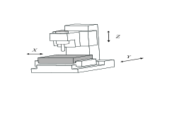
Figure 1: Typical industrial 3-axis machine-tool

For a $PPP$ topology, the kinematic equations are :

$${\bf{J}}\dot{\mbox{\boldmath${\rho}$\unboldmath}}={\bf\dot{p}}~{}~{}~{}~{}~{}{\rm with}~{}~{}~{}~{}~{}{\bf{J}}={\bf{1}}_{3\times 3}$$

where ${\bf\dot{p}}=[x~{}y~{}z]^{T}$ is the velocity-vector of the tool center point $P$ and ${\dot{\mbox{\boldmath${\rho}$\unboldmath}}}=[\rho_{1}~{}\rho_{2}~{}\rho_{3}]^{T}$ is the velocity-vector of the prismatic joints. The Jacobian kinematic matrix J being the identity matrix, the ellipsoid of manipulability of velocity and of force [1] is a unit sphere for all the configurations in the Cartesian workspace. The problem of the $PPP$ topology is that the actuator controlling the $Y$ axis supports at the same time the workpiece and the actuator controlling the displacement of the $X$ axis, which affects the dynamic performances. To solve this problem, it is possible to use more suitable kinematic architectures like parallel or hybrid topologies.

2.2 The Parallel Mechanisms Studied

We focus our study on the use of a 2-DOF parallel mechanism (Figure 3) for the motion of the table of the machine tool depicted in (Figure 1).

Figure 2: Two degree-of-freedom parallel mechanism

Figure 3: Two degree-of-freedom parallel mechanism with control of the orientation

The joint variables are the variables $\rho_{1}$ and $\rho_{2}$ associated with the two actuated prismatic joints and the output variables are the position of the tool center point $P=[x~{}y]^{T}$. The mechanisms can be parameterized by the lengths $L_{0}$, $L_{1}$ and $L_{2}$, the angles $\alpha_{1}$ and $\alpha_{2}$ and the actuated joint ranges $\Delta\rho_{1}$ and $\Delta\rho_{2}$ (Figure 3). To reduce the number of design parameters, we impose $L_{1}=L_{2}$ and $\Delta\rho_{1}=\Delta\rho_{2}$. This simplification also provides symmetry and, in turn, reduces the manufacturing costs.

To control the orientation of the reference frame attached to the tool center point $P$, two parallelograms can be used which also increase the rigidity of the structure (Figure 3).

2.3 Kinematics of the Parallel Mechanism Studied

The velocity ${\bf\dot{p}}$ of $P$ can be written in two different ways. By traversing the closed-loop $(ACP-BDP)$ in the two possible directions, we obtain

$${\bf\dot{p}}={\bf\dot{c}}+{\dot{\theta}}_{1}{\bf{E}}({\bf{p}}-{\bf{c}})$$ (1a)

and

$${\bf\dot{p}}={\bf\dot{d}}+{\dot{\theta}}_{2}{\bf{E}}({\bf{p}}-{\bf{d}})$$ (1b)

where E is the rotation matrix,

$${\bf{E}}=\left[\begin{array}[]{cc}0&-1\\ 1&0\end{array}\right]$$ (4)

c and d represent the position vector of the points $C$ and $D$, respectively.

Moreover, the velocity ${\bf\dot{c}}$ and ${\bf\dot{d}}$ of the points $C$ and $D$ are given by,

$${\bf\dot{c}}=\frac{{\bf{c}}-{\bf{a}}}{||{\bf{c}}-{\bf{a}}||}{\dot{\rho}}_{1}=\left[\begin{array}[]{c}\cos(\alpha_{1})\\ \sin(\alpha_{1})\end{array}\right]{\dot{\rho}}_{1}~{}~{}~{},~{}~{}~{}~{}{\bf\dot{d}}=\frac{{\bf{d}}-{\bf{b}}}{||{\bf{d}}-{\bf{b}}||}{\dot{\rho}}_{2}=\left[\begin{array}[]{c}\cos(\alpha_{2})\\ \sin(\alpha_{2})\end{array}\right]{\dot{\rho}}_{2}$$ (9)

The two unactuated joint rates ${\dot{\theta}}_{1}$ and ${\dot{\theta}}_{2}$ can be eliminated from equations (1a) and (1b) by dot-multiplying the former by ${\bf{p}}-{\bf{c}}$ and the latter by ${\bf{p}}-{\bf{d}}$, thus obtaining

$$({\bf{p}}-{\bf{c}})^{T}{\bf\dot{p}}=({\bf{p}}-{\bf{c}})^{T}\frac{{\bf{c}}-{\bf{a}}}{||{\bf{c}}-{\bf{a}}||}{\dot{\rho}}_{1}$$ (10a)

$$({\bf{p}}-{\bf{d}})^{T}{\bf\dot{p}}=({\bf{p}}-{\bf{d}})^{T}\frac{{\bf{d}}-{\bf{b}}}{||{\bf{d}}-{\bf{b}}||}{\dot{\rho}}_{2}$$ (10b)

Equations (2a) and (2b) can now be cast in vector form, namely,

$${\bf{A}}{\bf\dot{p}}={\bf{B}}\dot{\mbox{\boldmath${\rho}$\unboldmath}}$$

where A and B are, respectively, the parallel and serial Jacobian matrices, defined as

$${\bf{A}}=\left[\begin{array}[]{c}({\bf{p}}-{\bf{c}})^{T}\\ ({\bf{p}}-{\bf{d}})^{T}\end{array}\right]~{}~{}~{},~{}~{}~{}~{}{\bf{B}}=\left[\begin{array}[]{cc}({\bf{p}}-{\bf{c}})^{T}(({\bf{c}}-{\bf{a}})/||{\bf{c}}-{\bf{a}}||)&0\\ 0&({\bf{p}}-{\bf{d}})^{T}(({\bf{d}}-{\bf{b}})/||{\bf{d}}-{\bf{b}}||)\end{array}\right]$$ (15)

and with $\dot{\mbox{\boldmath${\rho}$\unboldmath}}$ defined as the vector of actuated joint rates and ${\bf\dot{p}}$ defined as the vector of velocity of point $P$:

$${\dot{\mbox{\boldmath${\rho}$\unboldmath}}}=\left[\begin{array}[]{c}{\dot{\rho}}_{1}\\ {\dot{\rho}}_{2}\end{array}\right]~{}~{}~{} ~{}~{}~{}~{}{\bf\dot{p}}=\left[\begin{array}[]{c}\dot{x}\\ \dot{y}\end{array}\right]$$ , (20)

When A and B are not singular, we can study the Jacobian kinematic matrix J [2],

$${\bf\dot{p}}={\bf{J}}{\dot{\mbox{\boldmath${\rho}$\unboldmath}}}~{}~{}~{}~{}{\rm with}~{}~{}~{}{\bf{J}}={\bf{A}}^{-1}{\bf{B}}$$ (21a)

or the inverse Jacobian kinematic matrix $${\bf{J}}^{-1}$$, such that

$${\dot{\mbox{\boldmath${\rho}$\unboldmath}}}={\bf{J}}^{-1}{\bf\dot{p}}~{}~{}~{}~{}{\rm with}~{}~{}~{}{\bf{J}}^{-1}={\bf{B}}^{-1}{\bf{A}}$$ (21b)

2.4 Parallel Singularities

The parallel singularities occur when the determinant of the matrix A vanishes [3, 4], i.e. when $\det({\bf{A}})=0$. In this configuration, it is possible to move locally the tool center point whereas the actuated joints are locked. These singularities are particularly undesirable, because the structure cannot resist any force and control is lost. To avoid any deterioration, it is necessary to eliminate the parallel singularities from the workspace.

For the mechanism studied, the parallel singularities occur whenever the points $C$, $D$, and $P$ are aligned (Figure 5), i.e. when $\theta_{1}-\theta_{2}=k\pi$, for $k=1,2,...$.

Figure 4: Parallel singularity

Figure 5: Structural singularity

They are located inside the Cartesian workspace and form the boundaries of the joint workspace. Moreover, structural singularities can occur when $L_{1}$ is equal to $L_{2}$ (Figure 5). In these configurations, the control of the point $P$ is lost.

2.5 Serial Singularities

The serial singularities occur when the determinant of the matrice B vanishes, i.e. when $\det({\bf{B}})=0$. When the manipulator is in such configurations, there is a direction along which no Cartesian velocity can be produced. The serial singularities define the boundary of the Cartesian workspace [Merlet 97].

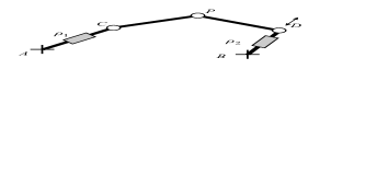
Figure 6: Serial singularity

For the topology studied, the serial singularities occur whenever $\theta_{1}-\alpha_{1}=\pi/2+k\pi$, or $\theta_{2}-\alpha_{2}=\pi/2+k\pi$, for $k=1,2,...$ (Figure 6), i.e whenever $AC$ is orthogonal to $CP$ or $BD$ is orthogonal to $DP$.

2.6 Application to Machining

For a machine tool with three axes as in (Figure 1), the motion of the table is performed along two perpendicular axes. The joint limits of each actuator give the dimension of the Cartesian workspace. For the parallel mechanisms studied, this transformation is not direct. The resulting Cartesian workspace is more complex and its size smaller. We want to have a Cartesian workspace which will be close to the Cartesian workspace of an industrial serial machine tool. For our 2-DOF mechanisms, we will prescribe a rectangular shape Cartesian workspace. In addition, the workspace must be reduced to a t-connected region, i.e. a region free of serial and parallel singularities [9]. Finally, we want to prescribe relatively stable kinetostatic properties in the workspace.

2.7 Velocity Amplification Study

In order to keep reasonable and homogeneous kinetostatic properties in the Cartesian workspace, we study the manipulability ellipsoids of velocity defined by the inverse Jacobian matrix ${\bf{J}}^{-1}$ [1]. For the mechanisms at hand, the inverse Kinematic Jacobian matrix ${\bf{J}}^{-1}$ given in equation (3b) is simple. In this case, the matrices B and ${\bf{J}}^{-1}$ are written simply,

$${\bf{B}}=\frac{1}{L_{1}}\left[\begin{array}[]{cc}1/c_{1}&0\\ 0&1/c_{2}\end{array}\right]~{}~{}{\rm and}~{}~{}{\bf{J}}^{-1}=\frac{1}{L_{1}}\left[\begin{array}[]{c}(1/c_{1})({\bf{p}}-{\bf{c}})^{T}\\ (1/c_{2})({\bf{p}}-{\bf{d}})^{T}\end{array}\right]~{}~{}{\rm with}~{}~{}c_{i}=\cos(\theta_{i}-\alpha_{i})~{}~{}i=1,2$$ (26)

The square roots $\gamma_{1}$ and $\gamma_{2}$ of the eigenvalues of $({\bf{J}}{\bf{J}}^{T})^{-1}$ are the values of the semi-axes of the ellipse which define the two factors of velocity amplification (from the joint rates to the output velocities), $\lambda_{1}=1/\gamma_{1}$ and $\lambda_{2}=1/\gamma_{2}$, according to these principal axes. To limit the variations of this factor in the Cartesian workspace, we pose the following constraints,

$$1/3<\lambda_{i}<3$$ (27)

This means that for a given joint velocity, the output velocity is either at most three times larger or, at least, three times smaller. This constraint also permits to limit the loss of rigidity (velocity amplification lowers rigidity) and of accuracy (velocity amplification also amplifies the encoder resolution). The values in equation (4) were chosen as an example and should be defined precisely as a function of the type of machining tasks.

3 Comparative Study

3.1 The Three Parallel Mechanism Architectures Studied

The three parallel mechanism architectures studied are the following:

1. The biglide1 mechanism with $\alpha_{1}=0$ and $\alpha_{2}=\pi$ (Fig. 7)

2. The biglide2 mechanism with $\alpha_{1}=\pi/2$ and $\alpha_{2}=\pi/2$ (Fig. 9)

3. The orthoglide mechanism with $\alpha_{1}=\pi/4$ and $\alpha_{2}=3\pi/4$ (Fig. 9)

The biglide1 mechanism studied (Fig. 7) has been used for example in the hexaglide and in the triglide [10].

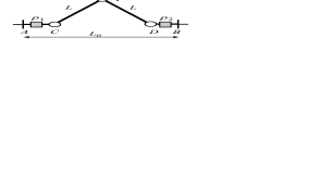
Figure 7: The biglide1 mechanism

The biglide2 mechanism (Fig. 9) has been used in the Linapod and in [10, 12].

Figure 8: The biglide2 mechanism

Figure 9: The orthoglide mechanism

The third mechanism (Fig. 9) was introduced in [11] and extended to 3-DOF in [10]. The main constraint of this design is $AC\perp BD$, which makes it isotropic, i.e. the Jacobian matrix of this mechanism is isotropic in some configurations.

3.2 Determination of the Mechanism Dimensions

To determine the mechanism dimensions, we proceed in several steps as follows. Let $L=L_{1}=L_{2}$ be the common link lengths, let $L_{0}$ be the distance between the attachment points A and B of the prismatic joints and let $\Delta\rho$ be the range of the actuated joints. The length $L_{0}$ and the joint range $\Delta\rho$ are determined consecutively as function of $L$ by using the condition on the velocity amplification factor (see section 2.7). For all mechanisms, we can show that the maximal (resp. minimal) velocity amplification factor is reached at the configuration for which the distance between C and D is maximal (resp. minimal). For the biglide1 and for the orthoglide, the maximal (resp. minimal) velocity amplification factor is reached at the configuration where C is on A and D is on B (resp. where C is on C’ and D is on D’) (figures 10 and 12).

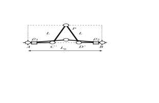
Figure 10: The biglide1 mechanism

Figure 11: The biglide2 mechanism

Figure 12: The orthoglide mechanism

By first writing that the maximal factor must be smaller than 3 in the first configuration, we can calculate $L_{0}$. Then $\Delta\rho$ is calculated by writing that in the opposite configuration the velocity amplification factor must be larger than 1/3. For the biglide2, the maximal (resp. minimal) amplification factor is reached at the configuration where C is on A and D is on D’(resp. where C and D lie on an horizontal line) (figure 12). In this case, we first calculate $L_{0}$ at the minimal factor configuration and $\Delta\rho$ is then calculated at the maximal factor configuration. The values of $L_{0}$ and $\Delta\rho$ obtained for all mechanisms are given in the first two rows of table 1. All derivations and computations have been obtained with MAPLE.

Mechanism	$L_{0}$	$\Delta\rho$	$S$
Biglide1	$1.946L$	$0.547L$	$0.107L$
Biglide2	$0.458L$	$0.529L$	$0.249L$
Orthoglide	$1.961L$	$1.109L$	$0.885L$

Table 1: Dimensions and rectangular Cartesian workspace surface as function of $L$

Then, for each mechanism, we determine the maximum rectangular surface $S$ which can be included in the Cartesian workspace (figures 15 to 15). We have used the parametric sketcher of a CAD system to perform this task. The area of the surfaces $S$ obtained are given in the last row of table 1. The last step is the scaling of the mechanism link dimensions and joint ranges in order to have a same Cartesian workspace rectangular for all mechanisms. The first three rows of table 2 give the resulting link dimensions and joint ranges.

Figure 13: The Cartesian workspace of the Biglide1

Figure 14: The Cartesian workspace of the Biglide2

Figure 15: The Cartesian workspace of the Orthoglide

3.3 Comparison of the Mechanism Size Envelopes

Table 2 provides the mechanism dimensions and envelope sizes for the three parallel mechanisms studied, for a prescribed rectangular Cartesian workspace surface of $1~{}m^{2}$.

Mechanism	$L_{0}$	$L$	$\Delta\rho$	Mechanism envelope surface
Biglide1	$5.95$	$3.05$	$1.67$	$16.45$
Biglide2	$0.92$	$2.00$	$1.06$	$8.50$
Orthoglide	$2.08$	$1.06$	$1.18$	$3.91$

Table 2: Mechanism dimensions and envelope sizes for a same rectangular Cartesian workspace

Figs. 16, 18 and 18 show the three mechanisms along with their Cartesian workspace and the same rectangular surface in it. We can notice that the orthoglide mechanism has smaller lengths struts i.e. smaller mass in motion and thus higher dynamic performances than the other two mechanisms. The biglide2 and the orthoglide mechanisms have similar values of $\Delta\rho$. It should be noticed, also, that the Cartesian workspace of the biglide2 includes a rectangulle which is far from a square, whereas it is an exact square for the other two mechanisms. We have calculated the dimensions of the biglide2 for a square of $1~{}m^{2}$ in its workspace and we have obtained $L_{0}=1.075$, $L=2.348$ and $\Delta\rho=1.242$.

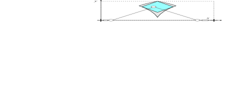
Figure 16: Workspace of the biglide1 mechanism

Figure 17: Workspace of the biglide2 mechanism

Figure 18: Workspace of the orthoglide mechanism

4 Conclusions

Three 2-DOF parallel mechanisms dedicated to machining applications have been compared in this paper. The link dimensions and the actuated joint ranges have been calculated for a same prescribed rectangular Cartesian workspace with identical kinetostatic constraints. The machine size of each resulting design was used as a comparative criterion. One of the mechanisms, the orthoglide, was shown to have lower dimensions than the other two mechanisms. This result shows that the isotropic property of the orthoglide induces interesting additional features like better compactness and lower inertia. In the future, the comparative study will be continued using dynamic performance indices.

References

- [1] Yoshikawa T., “ Manipulability and redundant control of mechanisms”, Proc. IEEE, Int. Conf. Rob. And Aut., pp. 1004–1009, 1985.
- [2] Merlet J.P., Les robots parallèles, 2nd édition, Hermès, Paris, 1997.
- [3] Chablat D., “Domaines d’unicité et parcourabilité pour les manipulateurs pleinement parallèles”, PhD Thesis, Nantes, Novembre, 1998.
- [4] Gosselin, C. and Angeles, J. “Singularity Analysis of Closed-Loop Kinematic Chains”, IEEE Trans. on Robotics and Automation, Vol. 6, No. 3, pp. 281–290, 1990.
- [5] Golub G.H. and Van Loan C.F., Matrix Computations, The John Hopkins University Press, Baltimore, 1989.
- [6] Wenger, P. Gosselin, C. and Maille. B. “A Comparative Study of Serial and Parallel Mechanism Topologies for Machine Tools”, Proc. PKM’99, Milano, pp. 23–32, 1999.
- [7] Kim, J. Park, C. Kim, J. and Park, F.C. 1997, “Performance Analysis of Parallel Manipulator Architectures for CNC Machining Applications”, Proc. IMECE Symp. On Machine Tools, Dallas.
- [8] Treib, T. and Zirn, O. “Similarity laws of serial and parallel manipulators for machine tools”, Proc. Int. Seminar on Improving Machine Tool Performance, pp. 125–131, Vol. 1, 1998.
- [9] Chablat, D. and Wenger, Ph. “On the Characterization of the Regions of Feasible Trajectories in the Workspace of Parallel Manipulators”, in Proc. Tenth World Congress on the Theory of Machines and Mechanisms, Vol. 3, pp. 1109–1114, Oulu, June, 1999.
- [10] Wenger, P. and Chablat, D. “Kinematic Analysis of a new Parallel Machine Tool: the Orthoglide”, in Lenarčič, J. and Stanišić, M.M. (editors), Advances in Robot Kinematic, Kluwer Academic Publishers, pp. 305–314, June, 2000.
- [11] Chablat D. Wenger P. and Angeles J., “Conception Isotropique d’une morphologie parallèle: Application l’usinage”, 3th Int. Conf. On Integrated Design and Manufacturing in Mechanical Engineering, Montreal, May 2000.
- [12] Horn, W. and Konold, T. “Parallelkinematiken für die Metallbearbeitung in der Automobil-Massenproducktion” Proc. Working Accuracy of Parallel Kinematics, Chemnitz, pp. 273–290, 2000.