26 July 2007

Neutrino production states in oscillation phenomena - are they pure or mixed?

Michał Ochman,  Robert Szafron,   and  Marek Zrałek

Department of Field Theory and Particle Physics,
Institute of Physics,

University of Silesia, Uniwersytecka 4, 40-007 Katowice, Poland
Tel: 048 32 2583653, Fax: 048 32 2588431

General quantum mechanical states of neutrinos produced by mechanisms outside the Standard Model are discussed. The neutrino state is described by the Maki-Nakagawa-Sakata-Pontecorvo unitary mixing matrix only in the case of relativistic neutrinos and Standard Model left-handed charge current interaction. The problem of Wigner spin rotation caused by Lorentz transformation from the rest production frame to the laboratory frame is considered. Moreover, the mixture of the neutrino states as a function of their energy and parameters from the extension of the Standard Model are investigated. Two sources of mixture, the appearance of subdominant helicity states, and mass mixing with several different mixing matrices are studied.

PACS :   13.15.+g, 14.60.Pq, 14.60.St

    Keywords:   neutrino oscillation, neutrino states, density matrix, Wigner rotation

1 Introduction

The neutrino oscillation phenomenon is well established. In several different experiments, the transition between different neutrino flavours is observed [1]. There is agreement that oscillation is possible when different mass neutrino states add coherently [2] in their production process. Such a combination of eigenmass neutrino states was defined many years ago by Maki, Nakagawa and Sakata [3] using the previous idea of neutrino mixing invented by Pontecorvo[4]. Now, there is agreement concerning the definition of so-called neutrino flavour states for relativistic neutrinos. The state of three massive relativistic neutrinos produced in the process involving a charged flavour $\alpha$ lepton is given by [5]

$$|\nu_{\alpha}\rangle=\sum_{i=1}^{3}U_{\alpha i}^{*}|\nu_{i}\rangle,$$ (1)

where $U$ is the unitary mixing matrix known as the Maki-Nakagawa-Sakata-Pontecorvo matrix. Such a state, which describes neutrinos with negative helicity, is understandable. Neutrinos are produced in charged lepton processes, which are described by the chiral left - handed interaction; the only one existing in the Standard Model (SM). Coupling of the charged $l_{\alpha}$ lepton with a massive $\nu_{i}$ neutrino and W boson is given by:

$$L_{CC}=\frac{e}{2\sqrt{2}\ sin\theta_{W}}\sum_{\alpha,i}\overline{\nu}_{i}\gamma^{\mu}(1-\gamma_{5})U_{\alpha i}^{*}l_{\alpha}W_{\mu}^{+}+h.c.$$ (2)

Such an interaction produces a relativistic neutrino with negative helicity (antineutrino with positive helicity), and its propagation in a vacuum or in matter does not reverse spin direction (neutral current interaction is also left-handed). In such circumstances, it is natural to describe neutrinos by a pure quantum mechanical state Eq.(1). So far, only relativistic neutrinos are detected (the detection energy threshold is practically larger then 100 keV [6]), and the pure production state Eq.(1) works well. However, there are several reasons to pose the following question about general neutrino states: What is the neutrino state if it is not necessarily relativistic, and/or its interaction is more general than that given by Eq.(2)? The answer for such a question is important as attempts are ongoing to define different neutrino states in a non-relativistic region (see e.g. [7] ). Besides, there is a chance that future more precise neutrino oscillation experiments will open a window for New Physics (NP) and the knowledge of the initial and final neutrino states could be important. The attempts to define general neutrino states have been discussed many times in the literature (see e.g.[8]). The neutrino production and detection states that depend on the specific physical process were considered in e.g. [9]. To our knowledge, the most general oscillation and detection neutrino states were studied by Giunti [10] (see also [11]). However, even in this work, only pure states in the relativistic case, without the spin effect of particles which produces neutrinos, are finally discussed.

The aim of our study is to construct a general neutrino density matrix using the helicity - mass basis using the amplitude for the production process in the CM system or rest system of a decaying object (e.g. muon in the neutrino factory or nucleus in the beta beam experiments) using a full wave packet description of particles. In order to find how physics beyond the SM modify neutrino production states, we consider the general neutrino interaction. Next, we transform the density matrix to the frame of the detector - the laboratory frame. Such a general Lorentz transformation causes Wigner rotation for spin states [12]. We show that, even if such a Wigner rotation can be large, its effect on neutrino helicity states is small and without practical meaning. Then we have the general density matrix describing a neutrino beam, which oscillates as it passes between the production site and the detector. In this way, we will be able, although it is not subject of this paper, to consider more precisely any possible influence of NP not only on oscillation phenomena as usual ([13]), but also on the production and, in a similar way, detection of neutrino. In such a case, all quantum mechanical properties of neutrino oscillation phenomena (such as the problem of factorization, oscillation and coherence length) could be considered in the more precise way.

We ask questions about when the neutrino state is pure and when it must be consider as mixed, how this property depends on neutrino energy, and the mechanism of the production process. We show that, for non-relativistic neutrinos, their state is always mixed. This is a very natural result, for neutrinos with an energy comparable to their masses, even a left-handed interaction (Eq.(2)) produces neutrinos with both helicities. Such a case must be described by a mixed state. But, as we will see, the appearance of the subdominant neutrino helicity states is not the only reason for the mixture of states. If the NP introduces different mixing matrices for different kinds of interactions (for vector and scalar couplings, as examples), quantum mixing of states also appears . Because of that, any attempt to treat a flavour neutrino as one object in Fock space (see e.g. [7]), even if mathematically consistent, creates a problem with the description of the real production process. Neutrino states are always mixed if the production mechanism is more complicated in comparison with the SM left-handed interaction Eq.(2). The neutrino density matrix also depends on the other properties of the production process; for example, the scattering angle, polarizations of other accompanying particles, and their momentum uncertainties as well as on the neutrinos themselves, the mass of the lightest neutrino, or their mass hierarchy.

In this paper, we discuss only the first stage of the oscillation process - the preparation of neutrino states - leaving the problem of oscillation, together with the interaction inside the medium and the problem of their detection, for a future paper. In the next Chapter, we describe the neutrino density matrix for the selected production process. As the base process, we take the neutrino production where charged flavour leptons $\alpha$ scatter on nuclei A ($l_{\alpha}+A\rightarrow\nu_{i}+B$). Amplitudes are calculated for the general interaction and the normalized ($Tr(\rho)=1$) density matrix in the CM system is found. Then, the problem of the Lorentz transformation and Wigner rotation is discussed. The full analytical and numerical properties of the neutrino density matrix are analyzed. To distinguish between mixed and pure states, we calculate $Tr(\rho^{2})$ as a function of neutrino energy and the parameters which describe the SM extensions. We also discuss how fast the neutrino states become pure as the energy increases. We study density matrices for two subsystems: the first which describes both neutrinos’ helicity independent of their mass, and the second describing the mixture of three neutrinos, independent of their spin state. Finally, Chapter 3 gives our final comments and future prospectives.

2 Neutrino states in the production processes

Let us assume that the beam of neutrinos with mass i, $\nu_{i}$ is produced by charged leptons $(\alpha=e,\mu)$ which scatter on nuclei A.

$$l_{\alpha}+A\rightarrow\nu_{i}+B.$$ (3)

We do not measure separate neutrinos and their masses; in fact, we do not directly measure neutrinos at all. Quantum neutrino states can be deduced from the measured states of all other particles accompanying the neutrino. So, having information about particles A, B and, especially, about charged lepton $l_{\alpha}$ in the process Eq.(3), gives us the ability to define neutrino states. To define the spatial or momentum distribution for neutrinos, we have to assume that all particles in the discussed process do not have a precisely determined momentum, so they must be defined by wave packets and not by plane waves (as is usually the case in other scattering processes). In order to discuss coherence effects in the detection process, we have to define the momentum distribution of the mass-helicity density matrix. Such a density matrix can be constructed from the amplitude for the process (3) whose interaction mechanism is under investigation.

We assume that our interaction is described by an effective model Lagrangian where both the vector and scalar couplings with the left and right chirality interaction are present. This sort of interaction appears, for example, in the Left - Right symmetric model (see e.g. [14]). We assume that:

$${\cal L}_{CC}= - \frac{e}{2\sqrt{2}sin\theta_{W}}\biggl{\{}\sum_{\alpha,i}\bar{\nu_{i}}\;[\;\gamma^{\mu}(1-\gamma_{5})\epsilon_{L}^{c}U_{\alpha i}^{L\ast}+\gamma^{\mu}(1+\gamma_{5})\epsilon_{R}^{c}U_{\alpha i}^{R\ast}]\;l_{\alpha}\;W^{+}_{\mu}$$ (4)

$$+ \sum_{\alpha,i}\bar{\nu_{i}}\;[\;(1-\gamma_{5})\eta_{L}V_{\alpha i}^{L\ast}+(1+\gamma_{5})\eta_{R}V_{\alpha i}^{R\ast}]\;l_{\alpha}\;H^{+}$$

$$+ \sum_{u,d}\bar{u}\;[\;\gamma^{\mu}(1-\gamma_{5})\epsilon_{L}^{q}U_{ud}^{\ast}+\gamma^{\mu}(1+\gamma_{5})\epsilon_{R}^{q}U_{ud}^{\ast}]\;d\;W^{+}_{\mu}$$

$$+ \sum_{u,d}\bar{u}\;[\;(1-\gamma_{5})\tau_{L}W_{ud}^{L\ast}+(1+\gamma_{5})\tau_{R}W_{ud}^{R\ast}]\;d\;H^{+}\biggr{\}}+h.c,$$

where $\varepsilon_{L,R}$, $\eta_{L,R}$ and $\tau_{L,R}$ are parameters that are taken to define the scale and differ slightly from their $\nu SM$ values.

In the neutrino sector, we introduce the mixing matrices separately for chiral-left and chiral-right parts as well as for vector and scalar neutrino interactions. As a consequence, phenomena such as flavour neutrino states, which were explicitly defined, do not exist any more, even for relativistic neutrinos. Mixing in the left-handed vector interaction $(U^{L})$ and left-handed scalar one $(V^{L})$ can be different and an unambiguous definition of flavour neutrino state is impossible. We see that the determination of the flavour neutrino state given by the Pontecorvo-Maki-Nakagawa-Sakata matrix is purely accidental and valid only in the SM and relativistic neutrino interaction. In such circumstances, we cannot consider flavour neutrinos as elementary quanta of a field theory.
In the lowest order, two Feynman diagrams describe the neutrino production process Eq.(3)

Figure 1: The charged boson(s) $W^{+}$ and charged Higgs particle(s) $H^{+}$ exchange diagrams, which describes the neutrino production process.

To define the neutrino state we have to calculate the amplitude for the process Eq. (3). Three measured particles $l_{\alpha}$, A and B are in the states given by the wave packets $(a=l,A,B)$

$$|\psi_{a},\lambda_{a}\rangle=\int d^{3}p_{a}\Psi_{a}(\vec{p}_{a},\vec{p}_{a0},\sigma_{ap})|\vec{p}_{a},\lambda_{a}\rangle,$$ (5)

where $|\vec{p}_{a},\lambda_{a}\rangle$ is the particle state with definite momentum $\vec{p}_{a}$ and helicity $\lambda_{a}$, and $\Psi_{a}(\vec{p}_{a},\vec{p}_{a0},\sigma_{ap})$ are the momentum distribution wave functions with a central momentum $\vec{p}_{a}$ and momentum uncertainty $\sigma_{ap}$. For A narrow momentum distribution ($\sigma_{ap}\ll|\vec{p}_{a}|$), the physical results are independent of the specific shape of these functions, and we take them in the Gaussian form:

$$\Psi_{a}(\vec{p}_{a},\vec{p}_{a0},\sigma_{ap})=\frac{1}{(2\pi\sigma_{ap}^{2})^{\frac{3}{4}}}e^{-\frac{(\vec{p}_{a}-\vec{p}_{a0})^{2}}{4\sigma_{ap}^{2}}}.$$ (6)

With such wave packet states, we calculate the amplitude for the process (3). After integration over the particles’ momenta we obtain:

$$\langle f|S|i\rangle=-i\frac{1}{[(2\pi\sigma_{lx}^{2})(2\pi\sigma_{Ax}^{2})(2\pi\sigma_{Bx}^{2})]^{\frac{3}{4}}}\int d^{4}xe^{-i(E-E_{R})t}e^{i(\vec{p}-\vec{p_{R}})\vec{x}}e^{-\frac{\vec{x}^{2}-2\vec{v}_{R}\vec{x}t+\Sigma_{R}t^{2}}{\sigma_{Rx}^{2}}}M(\vec{p},\lambda,...),$$ (7)

where the average values of neutrino energy and momentum are determined from the appropriate conservation rules (we use the same notation as in Ref ([10])):

$$E_{R}=E({\vec{p}}_{l0})+E({\vec{p}}_{A0})-E({\vec{p}}_{B0}^{\ i}),$$

and

$${\vec{p}}_{R}={\vec{p}}_{l0}+{\vec{p}}_{A0}-{\vec{p}}_{B0}^{\ i}.$$

For the precise energy and momentum determination we have to remember that, for a given total energy in the process (3), the final particle momenta and energies depend on the neutrino masses. The neutrino spatial uncertainty $\sigma_{Rx}$ and average velocity $\vec{v}_{R}$ are obtained from the accompanying particles uncertainties $\sigma_{ax}=\frac{1}{2\sigma_{ap}}$ and their velocities $\vec{v}_{a}=(\frac{dE}{d\vec{p}})_{\vec{p}=\vec{p}_{a}}$:

$$\frac{1}{\sigma^{2}_{Rx}}=\frac{1}{\sigma^{2}_{lx}}+\frac{1}{\sigma^{2}_{Ax}}+\frac{1}{\sigma^{2}_{1Bx}},$$

$${\vec{v}}_{R}=\sigma^{2}_{Rx}\left(\frac{{\vec{v}}_{l0}}{\sigma^{2}_{lx}}+\frac{{\vec{v}}_{A0}}{\sigma^{2}_{Ax}}+\frac{{\vec{v}}_{B0}}{\sigma^{2}_{Bx}}\right).$$

And, finally,

$${\Sigma}_{R}=\sigma^{2}_{Rx}\left(\frac{{\vec{v}}^{2}_{l0}}{\sigma^{2}_{lx}}+\frac{{\vec{v}}^{2}_{A0}}{\sigma^{2}_{Ax}}+\frac{{\vec{v}}^{2}_{B0}}{\sigma^{2}_{Bx}}\right).$$

The amplitudes $M(\vec{p},\lambda,...)\equiv M(\vec{p},\lambda;\lambda_{l},\lambda_{A},\lambda_{B})$ are the full helicity amplitudes for the production process Eq.(3), which is calculated in the CM frame for average values of all particle momenta except for the neutrino. Using the saddle-point approximation, the integrations over space and time can be done, giving the final amplitude $A^{\alpha}_{i}(\vec{p},\lambda,\lambda_{B};\lambda_{l},\lambda_{A})$ for the production of the $\nu_{i}$ neutrino with mass $m_{i}$, momentum $\vec{p}$, and helicity $\lambda$ in the process initiated by flavour $\alpha$ lepton:

$$A^{\alpha}_{i}(\vec{p},\lambda,\lambda_{B};\lambda_{l},\lambda_{A})\ =\ n_{\alpha i}\ f_{\alpha i}(\vec{p},E)\ M^{\alpha}_{i}(\vec{p},\lambda;\lambda_{l},\lambda_{A},\lambda_{B}),$$ (8)

where

$$n_{\alpha i}=\frac{2^{\frac{9}{4}}(\sigma_{lp}\ \sigma_{Ap}\ \sigma_{Bp})^{\frac{3}{2}}}{\pi^{\frac{1}{4}}\sigma_{Rp}^{4}\sqrt{\Sigma_{R}-v_{R}^{2}}},$$

and

$$f_{\alpha i}(\vec{p},E)=e^{-\frac{({\vec{p}}-{\vec{p}}_{R})^{2}}{4{\sigma}^{2}_{Rp}}-\frac{({\vec{v}}_{R}({\vec{p}}-{\vec{p}}_{R})-E+E_{R})^{2}}{\sigma^{2}_{Rp}\left({\Sigma}_{R}-{\vec{v}}^{2}_{R}\right)}},$$

where we have openly indicated that both factors depend on the neutrino mass. Once more, momentum uncertainty $\sigma_{Rp}=\frac{1}{2\sigma_{Rx}}$ appears in the above formulas. The second function $f_{\alpha i}$ describes the momentum distribution for the produced neutrinos.

The amplitude Eq.(8) describes all properties of the produced neutrinos. Their quantum mechanical state is determined by the density matrix defined as:

$$\varrho^{\alpha}(\vec{p},\ i,\ \lambda;\ \vec{p}^{\ {}^{\prime}},i^{{}^{\prime}},\lambda^{{}^{\prime}})=\frac{1}{N_{\alpha}}\sum_{\lambda_{l},\lambda_{A},\lambda_{B}}A^{\alpha}_{i}(\vec{p},\lambda,\lambda_{B};\lambda_{l},\lambda_{A})A^{\alpha*}_{i^{{}^{\prime}}}(\vec{p}^{\ {}^{\prime}},\lambda^{{}^{\prime}},\lambda_{B};\lambda_{l},\lambda_{A}),$$ (9)

where we assume that, in the production process (3), the initial particles are not polarized and the final polarization of the B nuclei is not measured. For the normalization factor $N_{\alpha}$, given by

$$N_{\alpha}=\sum_{\lambda=\pm 1}\sum_{i=1}^{3}\sum_{\lambda_{l},\lambda_{A},\lambda_{B}}\int d^{3}p|A^{\alpha}_{i}(\vec{p},\lambda,\lambda_{B};\lambda_{l},\lambda_{A})|^{2},$$ (10)

the density matrix is properly normalized:

$$Tr(\varrho^{\alpha})=\sum_{\lambda=\pm 1}\sum_{i=1}^{3}\int d^{3}p\ \varrho^{\alpha}(\vec{p},\lambda,i;\vec{p},\lambda,i)=1.$$ (11)

Eq. (9) describes the neutrino state in the CM frame. Such a frame is equivalent to the rest frame of a decaying muon in the neutrino factory case or the decaying nuclei in the beta beam experiments. Usually, neutrinos are not produced in such a frame. They are produced in the laboratory frame (LAB), where decaying muons or nuclei are moving very fast. The density matrix in such a frame is interesting for us. To reach the LAB frame, we have to make a Lorentz transformation. As helicity is not a full Lorentz scalar, we can expect that the density matrix in the LAB will be rotated (helicity Wigner rotation). Each neutrino state $|\vec{p},\lambda,i\rangle$ with mass $m_{i}$, momentum $\vec{p}$ and helicity $\lambda$ after a general Lorentz transformation $\Lambda$, does not necessary point along the neutrino momentum, but transforms as:

$$U[\Lambda]|\vec{p},s,\lambda\rangle=\sum_{\sigma}\textbf{D}^{s}_{\sigma\,\lambda}\Big{(}R^{T}(\varphi,\overline{\theta},-\varphi)R_{W}R(\varphi,\theta,-\varphi)\Big{)}|\Lambda\vec{p},s,\sigma\rangle,$$ (12)

where angles $\varphi$ and $\theta$ $(\varphi$ and $\overline{\theta})$ are the spherical angles of momenta before $(\vec{p})$ and after $(\Lambda\vec{p})$ which carry the Lorentz transformation. $R_{W}$ is the normal Wigner rotation:

$$R_{W}=L^{-1}(\Lambda\vec{p})\Lambda L(\vec{p}).$$ (13)

Hence, each element of the density matrix transforms as:

$$\varrho^{\alpha}(\vec{p},\ i,\ \lambda;\ \vec{p}^{\ {}^{\prime}},i^{{}^{\prime}},\lambda^{{}^{\prime}})\rightarrow\varrho^{\alpha}(\Lambda\vec{p},\ i,\ \eta;\ \Lambda\vec{p}^{\ {}^{\prime}},i^{{}^{\prime}},\eta^{{}^{\prime}})=$$ (14)

$$\,\,\,\,\sum_{\lambda\lambda^{{}^{\prime}}}\textbf{D}^{1/2}_{\eta\,\lambda}(R_{Wi}^{h})\,\varrho^{\alpha}(\vec{p},\ i,\ \lambda;\ \vec{p}^{\ {}^{\prime}},i^{{}^{\prime}},\lambda^{{}^{\prime}})\,\textbf{D}^{1/2*}_{\eta^{{}^{\prime}}\,\lambda^{{}^{\prime}}}(R_{Wi^{{}^{\prime}}}^{h}),$$

where $R_{Wi}^{h}$ is the helicity Wigner rotation:

$$R_{Wi}^{h}=R^{T}(\varphi,\overline{\theta},-\varphi)R_{W}R(\varphi,\theta,-\varphi),$$

and depends on neutrino mass as the neutrino momentum depends on it. The matrix $\textbf{D}^{1/2}_{\eta\,\lambda}(R_{Wi}^{h})$ can be found. If we parameterize:

$$\textbf{D}^{1/2}(R_{Wi}^{h})=\left(\begin{array}[]{cc}a&b\\ -b^{*}&a^{*}\\ \end{array}\right),$$ (17)

then

$$b=|b|e^{-i\varphi},$$

where

$$|b|=-\frac{S(\tilde{p}+C\tilde{E}\cos(\theta))-C\tilde{E}\sin(\theta)}{\sqrt{2[(\tilde{E}+\tilde{p}\cos(\theta))(\tilde{E}+C\tilde{p}+\tilde{p}\cos(\theta)+C\tilde{E}\cos(\theta)+S\tilde{E}\sin(\theta))]}},$$

$$a=\sqrt{1-|b|^{2}},$$

and

$$\tilde{p}=p\beta\gamma,\,\,\,\,\tilde{E}=m_{i}+E\gamma,$$

with

$$C=\frac{\gamma(E\beta+p\cos(\theta))}{\sqrt{\gamma^{2}(E\beta+p\cos(\theta))^{2}+p^{2}\sin^{2}(\theta)}},\,\,\,\,\,S=\sqrt{1-C^{2}}.$$

Here $m_{i},E$ and $p$ are the neutrino mass, energy and momentum, $\gamma$ and $\beta$ are parameters of the Lorentz transformation in the ”z” direction, and $\theta,\varphi$ are spherical angles of the neutrino momentum.

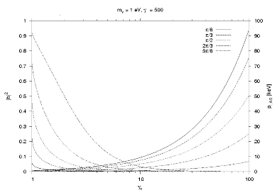
Figure 2: On the left - the off-diagonal element $|b|$ of the helicity Wigner rotation matrix as a function of the neutrino’s $\gamma_{\nu}=\frac{E}{\,m_{i}}$ factor for five different neutrino scattering angle $\theta=\frac{\pi}{6},\frac{\pi}{3},\frac{\pi}{2},\frac{2\pi}{3}$ and $\frac{5\pi}{6}$ in CM. The Lorentz transformation is described by the $\gamma=500$ factor. On the right side, the neutrino momentum in LAB system for the same scattering angle in the CM frame is shown.

It is worth noticing that, for normal (not helicity) Wigner rotation $R_{W}$, $C\rightarrow cos\theta$ and $S\rightarrow sin\theta$. The off-diagonal element of the $D^{1/2}$ matrix Eq.(17) b decides how big the effect of the Wigner rotation is. In Fig. 2, on the left side, we have plotted the $|b|$ element as a function of neutrino $\gamma$ factor ($\gamma_{\nu}=\frac{E}{m_{i}}$) for various scattering angles $\theta_{CM}$ for the Lorentz transformation along the ”z” axis with $\gamma=500$. We see that the effect is large but only for very small neutrino energies ($E\approx m_{i}$) and large scattering angles. Unfortunately, as we see from right side of the picture, such neutrinos also have small energies in LAB frame and are not measured. The effect of the helicity flip for experimentally measurable neutrinos with a enough large energy ($E_{LAB}\gtrsim 100$ MeV) is completely negligible. We see that, for practical purposes, we can safely take it that Lorentz transformation does not change the helicity structure of the density matrix and

$$\varrho^{LAB}(\Lambda\vec{p},\ i,\ \lambda;\ \Lambda\vec{p}^{\ {}^{\prime}},i^{{}^{\prime}},\lambda^{{}^{\prime}})=\,\,\,\,\varrho^{CM}(\vec{p},\ i,\ \lambda;\ \vec{p}^{\ {}^{\prime}},i^{{}^{\prime}},\lambda^{{}^{\prime}}).$$ (18)

We can now check the quantum structure of the neutrino state described by Eq.(9). First, we would like to answer how good the MNSP assumption (Eq.(1)) is. In order to do that, we calculate $Tr[(\varrho^{\alpha})^{2}]$:

$$Tr[(\varrho^{\alpha})^{2}]=\sum_{\lambda\,i\,\lambda^{{}^{\prime}}i^{{}^{\prime}}}\int d^{3}p\ \,d^{3}p^{\,{}^{\prime}}\varrho^{\alpha}(\vec{p},\ i,\ \lambda;\ \vec{p}^{\ {}^{\prime}},i^{{}^{\prime}},\lambda^{{}^{\prime}})\varrho^{\alpha}(\vec{p}^{\ {}^{\prime}},i^{\ {}^{\prime}},\lambda^{{}^{\prime}};\ \vec{p},\ i,\ \lambda),\,$$ (19)

and check how it differs from unity.

To be more precise and to not complicate our consideration with the structures of particles A and B, which are not important for our purpose, we take the u and d quarks with masses $m_{u}=2.25\ MeV$ and $m_{d}=5.0\ MeV$ as particles A and B, respectively. For lepton $\alpha$ we take an electron with $m_{e}=0.511\ MeV$. All Particles’ momenta uncertainties are equal and $\sigma_{ep}=\sigma_{up}=\sigma_{dp}=10\ eV$. The results do not depend crucially on the values of these uncertainties.

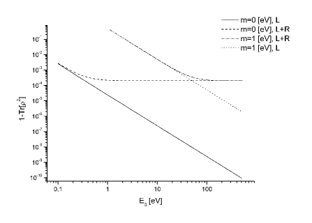
Figure 3: $1-Tr[\rho^{2}]$ as a function of the neutrino kinetic energy for the two lightest neutrino mass $m_{1}=0\ eV$ and $m_{1}=1\ eV$ with only Left ($\varepsilon_{L}=1,\varepsilon_{R}=0.)$ and the Left- and Right-currents ($\varepsilon_{L}=1,\varepsilon_{R}=0.01$).

In Fig. 3, we plot $1-Tr[(\varrho^{\alpha})^{2}]$ as a function of the kinetic neutrino energy for two values of the lightest neutrino mass, $m_{1}=0\ eV$ and $m_{1}=1\ eV$ in two cases, when only Left-Handed chiral interactions are present (only $\varepsilon_{L}\neq 0$), and when Left- and Right-current exist ($\varepsilon_{L}\neq 0$ and $\varepsilon_{R}\neq 0$). The masses of the heavier neutrinos and the vector Left-Handed mixing ($U_{L}$) are taken from the oscillation data [15]. We assume a normal mass hierarchy with $m^{2}_{\odot}$ = $8.0\times 10^{-5}eV^{2}$, $m^{2}_{atm}$ = $2.5\times 10^{-3}eV^{2}$ and mixing angles, $sin^{2}\theta_{12}=0.31,\,sin^{2}\theta_{23}=0.44,\,sin^{2}\theta_{13}=0.009$ and $\delta_{CP}=0$ (central values are taken). The mixing in the Right-Handed vector ($U_{R}$) and scalar interactions ($V_{L,R}$) we take to be the same as in the L-H case ($V_{L}=V_{R}=U_{R}=U_{L}$). As we will see, by taking the same mixing matrices, we ignore the QM mixing caused by different mass states, and assume possible mixing effects are caused only by different helicity states. If the production process is described by the SM interaction (only L-H vector interaction), the state is strongly mixed for very small neutrino energies (continuous line and dotted line). The effect of the mixture depends on the lightest neutrino mass (as we see from the Fig. 3) and depends also slightly on the mass hierarchy and chosen particle momentum uncertainties (not shown).

If the neutrinos’ energies increase, their state becomes pure. For relativistic neutrinos where masses and momentum uncertainties can be neglected, the density matrix takes the form:

$$\varrho^{\alpha}(+1,i;+1,k)=\frac{1}{N_{\alpha}}\big{(}A_{\varepsilon_{R}^{2}}\,\varepsilon_{R}^{2}\,U_{\alpha i}^{R*}U_{\alpha k}^{R}+A_{\eta_{L}^{2}}\,\eta_{L}^{2}\,V_{\alpha i}^{L*}V_{\alpha k}^{L}+A_{\varepsilon_{R}\eta_{L}}\,\varepsilon_{R}\eta_{L}\,(U_{\alpha i}^{R*}V_{\alpha k}^{L}+V_{\alpha i}^{L*}U_{\alpha k}^{R})\big{)},$$ (20)

$$\varrho^{\alpha}(+1,i;-1,k)=\varrho^{\alpha}(-1,k;+1,i)^{*}=$$ (21)

$$\frac{1}{N_{\alpha}}\big{(}A_{\varepsilon_{L}\varepsilon_{R}}\,\varepsilon_{R}\varepsilon_{L}\,U^{R*}_{\alpha i}U^{L}_{\alpha k}+A_{\varepsilon_{R}\eta_{R}}\,\varepsilon_{R}\eta_{R}\,U^{R*}_{\alpha i}V^{R}_{\alpha k}+A_{\varepsilon_{L}\eta_{L}}\,\varepsilon_{L}\eta_{L}\,V^{L*}_{\alpha i}U^{L}_{\alpha k}\big{)},$$

$$\varrho^{\alpha}(-1,i;-1,k)=\frac{1}{N_{\alpha}}\big{(}A_{\varepsilon_{L}^{2}}\,\varepsilon_{L}^{2}\,U_{\alpha i}^{L*}U_{\alpha k}^{L}+A_{\eta_{R}^{2}}\,\eta_{R}^{2}\,V_{\alpha i}^{R*}V_{\alpha k}^{R}+A_{\varepsilon_{L}\eta_{R}}\,\varepsilon_{L}\eta_{R}\,(U_{\alpha i}^{L*}V_{\alpha k}^{R}+V_{\alpha i}^{R*}U_{\alpha k}^{L})\big{)},$$ (22)

and

$$\ \ N_{\alpha}=A_{\varepsilon_{L}^{2}}\,\varepsilon_{L}^{2}\,+A_{\eta_{R}^{2}}\,\eta_{R}^{2}\,+A_{\varepsilon_{R}^{2}}\,\varepsilon_{R}^{2}\,+A_{\eta_{L}^{2}}\,\eta_{L}^{2}\,+$$ (23)

$$A_{\varepsilon_{R}\eta_{L}}\,\varepsilon_{R}\eta_{L}\,(V^{L}U^{R{\dagger}}+U^{R}V^{L{\dagger}})_{\alpha\alpha}+A_{\varepsilon_{L}\eta_{R}}\,\varepsilon_{L}\eta_{R}\,(V^{R}U^{L{\dagger}}+U^{L}V^{R\dagger})_{\alpha\alpha},$$

where the A factors (not given here) depend on the neutrino energy and scattering angles. We see that, in the SM where only $\varepsilon_{L}\neq 0$:

$$\varrho^{\alpha}(-1,i;-1,k)=U_{\alpha i}^{L*}U_{\alpha k}^{L},$$ (24)

and all other elements of density matrix are equal zero. Such a density matrix describes pure states equivalent to the MNSP mixture Eq. (1). Relativistic neutrinos in the SM model are produced in the pure states described by the MNSP mixture. The situation changes if any NP participates in the neutrino production process. Then, the states are not pure - even for relativistic neutrinos. A departure from the pure state depends on two properties of the system: the helicity mixing and the mass mixing. The first is obvious - neutrinos in two helicity states are produced which, in a natural way, gives the mixed state. The second effect is more mysterious and appears only if the mixing matrices are not the same. In order to investigate both effects, we can construct separately two density matrices for two subsystems - the first for the helicity subsystem and the second for the mass. For the helicity subsystem, the density matrix is given by:

$$\varrho^{\alpha,spin}_{\lambda,\eta}=\sum_{i=1}^{3}\varrho^{\alpha}(\lambda,i;\eta,i),$$ (25)

and, for the mass subsystem:

$$\varrho^{\alpha,mass}_{i,k}=\sum_{\lambda=\pm 1}\varrho^{\alpha}(\lambda,i;\lambda,k).$$ (26)

With reference to the helicity subsystem, $1-Tr[(\varrho^{\alpha,spin})^{2}]$ is different then zero even if all mixing matrices are equal, and it is a second order effect in the NP parameters:

$$1-Tr[(\varrho^{\alpha,spin})^{2}]\approx O(\varepsilon_{R}^{2},\eta_{R}^{2},\eta_{L}^{2}).$$

In Fig. 3, we see (dashed line $(m_{1}=0\,eV)$ and dashed - doted line $(m_{1}=1\,eV)$ that above the non-relativistic region, where even the L-H vector current produces neutrinos with h=+1/2, the state mixture is almost constant and of the order of $\varepsilon_{R}^{2}\approx$ 0.0001. Generally, the mixture of the neutrino states is, in a good approximation, proportional to the probability squared that neutrinos with negative helicity are produced.

$$Tr[(\varrho^{\alpha})^{2}]\approx(Tr[\varrho^{\alpha}\widehat{P}_{-}])^{2},$$ (27)

where the $\widehat{P}_{-}$ is the projection operator on the negative helicity state, $(\widehat{P}_{-})_{\lambda,\,i\,;\,\eta,\,k}=\delta_{\lambda,-1}\delta_{\eta,-1}\delta_{i,k}$.

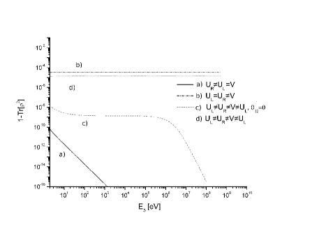
Figure 4: 1-$Tr[(\varrho^{\alpha,mass})^{2}]$ as a function of the kinetic neutrino energy for various mixing matrices in the vector and scalar Lagrangian. For the parameter which defines New Physics, we take $\varepsilon_{R}=0.01,\eta_{L}=\eta_{R}=0.02$. All matrices are parameterized in the same way as the standard $U_{L}$ matrix.   a) $sin^{2}\theta_{12}=0.87,sin^{2}\theta_{23}=0.09,sin^{2}\theta_{13}=0.23$, $\delta_{CP}=0.5$ for $U_{R}$ and $V_{L}=V_{R}=U_{L}$;   b) $V_{L}=V_{R}$ as $U_{R}$ in the case a) and $U_{R}=U_{L}$;   c) $V_{L}=V_{R}$ the same as in b) and $sin^{2}\theta_{12}=0,sin^{2}\theta_{23}=0.09,sin^{2}\theta_{13}=0.71$, $\delta_{CP}=0.8$ for $U_{R}$;   d) $V_{L}=V_{R}$ as in the case b) and $sin^{2}\theta_{12}=0.01,sin^{2}\theta_{23}=0.09,sin^{2}\theta_{13}=0.71$, $\delta_{CP}=0.8$ for $U_{R}$.

In Fig. 4, we depicted the effect of neutrino state mixtures caused by the mass mixing. First, for relativistic neutrinos, there is no mixture if all mixing matrices are the same:

$$Tr[(\varrho^{\alpha,mass})^{2}]=1,$$

if $U_{R}=V_{R}=V_{L}=U_{L}$. We see also that the size of the mixture depends on the shape of the chosen mixing matrices. For some mixing matrices, the mixture can be large and of the order of $O(\varepsilon_{R}^{2},\eta_{R}^{2},\eta_{L}^{2})$.

Both sources of state mixtures, helicity mixing and mass mixing, can have comparable effects. For example, the dotted-dashed line in Fig. 4, where we take $U_{R}=U_{L}\neq V_{L}=V_{R}$, indicates that the departure of $Tr[(\varrho^{\alpha,mass})^{2}]$ from unity is maximal. Here, we parameterize the V matrices in the same way as the standard $U_{L}$ matrix and take $sin^{2}\theta_{12}=0.87,sin^{2}\theta_{23}=0.09,sin^{2}\theta_{13}=0.23$ and $\delta_{CP}=0.5$. If, instead, we take $V_{L}=V_{R}=U_{L}\neq U_{R}$ (the continuous line in Fig. 4), the mixture caused by mixing between different states of neutrino masses is marginal. The neutrino mixing in the scalar sector has a decisive role.

3 Conclusions

We have constructed the density matrix for neutrinos created in any production process. Numerical calculations have been performed for the elementary reaction $e^{-}+u\rightarrow\nu_{i}+d$. The density matrix has been calculated in the total Center of Mass system. Beyond this, we have shown that the Lorentz transformation to Laboratory system (the rest frame of a detector) has negligible effects on the density matrix for experimentally interesting neutrinos. For neutrinos with energies close to their masses, their states must be described by a mixed density matrix. In this region, the effect depends on the lightest neutrino mass, the mass hierarchy, and the particles’ momenta uncertainties given in wave packets. It was shown that, for relativistic neutrinos, mixing of the states depends on the mechanism of the production process. For the $\nu SM$, where only a Left-Handed vector current is in effect, neutrinos are produced in a pure state with extreme accuracy. In this way, the assumption about so-called flavour states as in the Maki-Nakagawa-Sakata-Pontecorvo mixture of the mass states, is justified. If NP interactions also influence the neutrino production process, the assumption about purity of neutrino production states is not legitimate. Departure from pure states is caused by two things: the possible production of neutrinos in two helicity states caused, for example, by Right-Handed currents or by scalar interactions, and by their mixing given by different mixing matrices in the various sectors of the production mechanism. Separate density matrices for the helicity subsystem and mass subsystem were constructed. Both of these effects have been investigated numerically and analytically in the case of relativistic and non-relativistic neutrinos.

Acknowledgments: This work has been partially supported by the Polish Ministry of Science under grant No.1 P03 B 049 26, and by the European Community’s Marie-Curie Research Training Network under contract MRTN-CT-2006-035505 ”Tools and Precision Calculations for Physics Discoveries at Colliders”

References

- [1] Fukuda, Y. et al. (Super-Kamiokande), Phys. Rev. Lett. 81 (1998) 1562-1567; Davis, R., Prog. Part. Nucl. Phys. 32 (1994) 13-32; Hosaka, J. et al. (Super-Kamkiokande), Phys. Rev. D73 (2006) 112001; Phys. Rev. Lett. 89 (2002) 011301.
- [2] B. Kayser, Phys. Rev. D 24 (1981) 110.
- [3] Z. Maki, M. Nakagawa and S. Sakata, Prog.Theor. Phys. 28 (1962) 870.
- [4] B. Pontecorvo, J. Expetl. Theoret. 33 (1957) 549 and ibid. 34 (1958) 247.
- [5] S. Eliezer and A.R. Swift, Nucl. Phys. B105 (1976) 45; H. Fritzsch and P. Minkowski, Phys.Lett. B62 (1976) 72; S.M. Bilenky and B. Pontecorvo, Sov. J. Nucl.Phys. 24 (1976) 316; S.M. Bilenky and B. Pontecorvo, Nuovo Cim. Lett. 17 (1976) 569.
- [6] see e.g. S. Bilenky, C. Giunti and W. Grimus, Prog. Part. Nucl. Phys. 43 (1999) 1.
- [7] M.Blasone, G.Vitiello, Annals Phys. 244 (1995) 283; Blasone, P.A.Henning and G. Viliello, Phys.Lett.B 451 (1999) 140; K.Fujii, C.Habe and T. Yabuki, Phys.Rev. D59 (1999) 113003 and Phys.Rev.D64 (2001) 013011; M.Binger and C.R.Ji, Phys.Rev. D60 (1999) 056005; C.R.Ji and Y.Mishchenko, Phys.Rev. D64 (2001) 076004; D.Boyanovsky and C.M.Ho, Phys.Rev D69 (2004) 125012.
- [8] Kiers, N. Weiss, Phys. Rev. D57 (1998) 3091; C. Giunti, J.Phys. G34 (2007) 93; C.Giunty, Eur. Phys. J. C39 (2005) 377.
- [9] Y.Grossman, Phys.Lett. B359 (1995) 141.
- [10] C. Giunti, JHEP 0211 (2002) 017.
- [11] M. Beuthe, Phys.Rept. 375 (2003) 105; Ch. Cardall, Phys.Rev. D61 (2000) 073006; M. Zralek, Acta Phys. Polon. B29 (1998) 3925.
- [12] E. P. Wigner, Ann. Math. 40, 149 (1939) 204.
- [13] C. Giunti, C. W. Kim and U. W. Lee, Phys. Lett. B 274 (1992) 87; Y. Takeuchi, Y. Tazaki, S. Y. Tsai, T. Yamazaki, Prog. Theor. Phys. 105 (2001) 471-482; M. Nauenberg, Phys. Lett. B447 (1999) 23-30.
- [14] J.C. Pati and A. Salam,Phys.Rev. D10 (1974) 277; R.N. Mohapatra and J.C. Pati, Phys.Rev. D11 (1975) 2558; G. Sanjanovic, Nucl.Phys Nucl. Phys. B153 (1979) 334; P.Duka, J. Gluza and M. Zralek, Annals of phys. 280 (2000) 336.
- [15] G.L. Fogli et all, Prog.Part.Nucl.Phys. 57 (2006) 742-795.