Forecasting the Evolution of Dynamical Systems from Noisy Observations

Abstract

We consider the problem of designing almost optimal predictors for dynamical systems from a finite sequence of noisy observations and incomplete knowledge of the dynamics and the noise. We first discuss the properties of the optimal (Bayes) predictor and present the limitations of memory-free forecasting methods, and of any finite memory methods in general. We then show that a nonparametric support vector machine approach to forecasting can consistently learn the optimal predictor for all pairs of dynamical systems and bounded observational noise processes that possess summable correlation sequences. Numerical experiments show that this approach adapts the memory length of the forecaster to the complexity of the learning task and the size of the observation sequence.

Our goal is to design almost optimal predictors for dynamical systems conditioned only on a finite sequence of observed noisy measurements of its evolution and imperfect knowledge of the dynamics and noise. Suppose that $F:X\to X$ is a map on a compact subset $X\subset\mathbb{R}^{d}$ such that the associated dynamical system ${\mathcal{D}}:=(F^{i})_{i\geq 0}$, where $F^{i}=F\circ F^{i-1}$, has an ergodic measure $\mu$. For example, if $X$ is compact and $F$ is continuous such a measure always exists. Moreover, let ${\mathcal{E}}:=(\varepsilon_{i})_{i\geq 0}$ be an $\mathbb{R}^{d}$-valued i.i.d. process with respect to the distribution $\nu$ that is independent of the process ${\mathcal{D}}$. We assume that all observations of the dynamical system are perturbed by the process ${\mathcal{E}}$, i.e. all observations are of the form

$$z_{i}:=F^{i}(x_{0})+\varepsilon_{i}\,,$$ (1)

where $x_{0}$ is the unknown initial point of the trajectory. Let us now assume that we have a sequence of observations $z_{1},\dots,z_{m}$ and we wish to predict the observation $z_{m+l}$, or the true state $x_{m+l}$, after some time $l$ as best as possible. Then one possible formalization of this problem is to look for a minimizer $f^{*}_{m,l}$, called the Bayes forecaster, of the risk functional

$${{\cal R}_{m,l}(f)}=\int_{\mathbb{R}^{d}}\int_{\mathbb{R}^{(m+1)d}}\bigl{\|}F^{m+l}(x)+\varepsilon_{m+l}$$ (2)

$$-f\bigl{(}F(x)+\varepsilon_{1},\dots,F^{m}(x)+\varepsilon_{m}\bigr{)}\bigr{\|}_{p}^{p}\,\nu^{m+1}(d\varepsilon)\mu(dx)\,,$$

which describes the average discrepancy (measured in the $\|\cdot\|_{p}$-norm) between the predictions of $f:\mathbb{R}^{md}\to\mathbb{R}^{d}$ and the observations (we have made a time-shift by $m+1$ in order to handle non-invertible maps $F$). To attain this goal we want to design a learning method $\cal{L}$, which assigns to each observed trajectory $T_{n}=\{z_{0},\dots,z_{n}\}$, $n\geq m$, a forecaster $f_{T_{n}}$ and which is consistent, i. e.

$$\lim_{n\to\infty}{{\cal R}_{m,l}(f_{T_{n}})}={{\cal R}_{m,l}^{*}}$$ (3)

holds in probability, where ${{\cal R}_{m,l}^{*}}={{\cal R}_{m,l}(f_{m,l}^{*})}$ is the minimum risk (the Bayes risk).

Most classical forecasting methods use a Markov state-space approach to modeling dynamic systems and require a model of both the flow $F$ and the observational noise $\nu$. These methods usually attempt to estimate the probability density function (PDF) of the state based on all the available information, i. e. $p(X_{m}|Z_{1}^{m})$, where $Z_{1}^{m}:=(Z_{1},\dots,Z_{m})$ and $(Z_{i})$ denotes the stochastic process that generates the observations. Then, an optimal (with respect to any criterion) forecaster may be obtained from the PDF, including $\mathbb{E}(X_{m+l}|Z_{1}^{m})=\int p(X_{m}|Z_{1}^{m})F^{l}(X_{m})dX_{m}$. Known as nonlinear filters, these methods estimate recursively in time this distribution and consist of essentially two steps: a prediction step, that uses the system model to propagate the state PDF to the next observation time, and an update step, that uses the latest observation to modify the prediction PDF using Bayes’ rule. Except in a few special cases, including linear Gaussian state space models (Kalman filter) and hidden finite-state space Markov chains, the recursive propagation of the posterior PDF cannot be determined analytically Maybeck (1979). Consequently, various approximations strategies to the optimal solutions have been developed. The most popular algorithms, the extended and the unscented Kalman filter, rely on anlytical approximations of the flow or/and finite moment approximations of the posterior PDF. Alternatively, sequential Monte Carlo methods, have conceptually the advantage of not being subject to the assumptions of linearity or Gaussianity in the model, but are computationally very expensive and suffer from the degeneracy of the algorithm Doucet et. al. (2000).

Notwithstanding their significant merits, there are many difficulties in these approaches to forecasting. First, due to their reliance on system and noise models they are sensitive to model errors. Second, instead of solving the function estimation problem directly, for which the available information might suffice, they estimate densities as a first step, which is a harder and more general problem that requires a large number of observations to be solved well. Third, by relying on a Markov state-space approach to forecasting they heavily restrict the class of functions available for forecasting. In order to further appreciate this aspect, and to better understand our proposed approach, let us now describe the structure of the optimal forecasters in more detail for the special case $p=2$. If the noise has no systematic bias, i.e. $\mathbb{E}_{\nu}\varepsilon_{i}=0$, simple algebra then shows that $f^{*}_{m,l}$ is not only the optimal forecaster for the observable state $z_{m+l}$ but also for the true state $x_{m+l}$. Moreover, it is well known that $f^{*}_{m,l}=\mathbb{E}(Z_{m+l}|Z_{1}^{m})$, but this closed form does in general not solve the issue of actually computing $f_{m,l}^{*}$ since for many cases this computation is intractable even with perfect knowledge of $F$, $\mu$ and $\nu$. However, if the noise has a density $\vartheta$ with respect to the Lebesgue measure, $f^{*}_{m,l}$ can be expressed by a more tractable formula,

$$f_{m,l}^{*}(z_{1},\ldots,z_{m})=$$ (4)

$$\frac{\int_{\mathbb{R}^{d}}\vartheta(z_{1}-F(x))\cdots\vartheta(z_{m}-F^{m}(x))F^{m+l}(x)d\mu(x)}{\int_{\mathbb{R}^{d}}\vartheta(z_{1}-F(x))\cdots\vartheta(z_{m}-F^{m}(x))d\mu(x)}\,.$$

When perfect knowledge of the system is available, the above equation describes how to build the optimal predictor. Even though these assumptions are rarely met in practice the above result points to a number of interesting and very general conclusions with regard to forecasting the future of a dynamical system based on noisy observations:

1) In general the flow $F$ is not the optimal predictor. Indeed Eq. (4) clearly shows that the flow $F$ is in general not the optimal one-step predictor based only on a noisy estimate of the present state of the system, i.e. $F\neq f^{*}_{1,1}$. A good example is provided by the logistic map, defined as $F(x)=1-ax^{2},$ $x\in[-1,1]$, which is known to be ergodic and has an invariant measure given by $\mu(x)=1/\pi(1-x^{2})^{1/2}$ Beck and Schlögl (1993). As we can clearly see from Fig. (1), the true dynamical behavior $F$ (continuous line) and the best forecaster $f_{1,1}^{*}$ (dashed line) disagree. However, in the absence of observational noise, we obviously obtain $F=f^{*}_{1,1}$ from Eq. (2), i.e. $F$ is the optimal, memoryless, one-step ahead predictor.

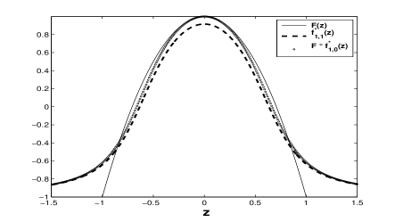
Figure 1: Comparison of three, memoryless, forecasting strategies for one-step ahead predictions for the logistic map and large Gaussian noise ($\sigma=0.2$): the true dynamical behavior, $F$ (continuous line), the best forecaster (dashed), and $F$ composed with the best memory-free denoiser, $f^{*}_{1,0}$ (dotted).

2) Recursive forecast is worse than direct forecast. Since in general for $l$ step ahead predictors we have $f_{m,l}^{*}\neq(f_{m,1}^{*})^{l}$ we see that iterating one-step-ahead forecasts is in general worse than directly forecasting $l$-steps ahead. In Fig. (2), where we plot the direct two-step ahead forecaster as well as the recursive forecaster obtained by iterating the optimal one-step ahead Bayes predictor, illustrates this effect for the logistic map. In general, as the forecasting time increases the iterated forecasters become more and more inadequate. Of course, for noiseless observations direct and recursive predictors have the same forecasting performance.

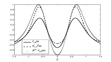
Figure 2: Comparison of the direct (continuous line) and recursive forecaster (dashed line) for two-step ahead predictors for the logistic map with large Gaussian noise with $\sigma=0.2$. Also shown is $F^{2}$ composed with the best memory-free denoiser, $f^{*}_{1,0}$ (dotted line).

3) Forecasts based on denoising the present state are not optimal. By choosing $l=0$ in Eq. (4) we obtain an optimal estimate (optimal denoiser) of the present state of the dynamical system based on a history of length $m$ rem . Now a common forecasting strategy is to estimate the present system state first and then apply the dynamics $F^{l}$ to this estimate. It should be is clear from our discussion so far that even if the estimate of the present state is optimal it still approximates the true state: therefore, this forecaster is not the optimal $l$-step ahead forecaster based on histories of length $m$. The dotted line in Fig. (1), which is $F$ composed with the best memory-free denoiser, $f^{*}_{1,0}$, and the one in Fig. (2), which is $F^{2}$ composed with $f^{*}_{1,0}$, illustrate the principal limit of memory-free, and of any finite memory denoising, followed by propagating the dynamics.

4) Memory improves forecasting performance. Indeed, building one-step ahead predictors using the past $m$ states is a minimization of the risk functional over the space of all measurable functions $f:\mathbb{R}^{m}\to\mathbb{R}$. This function space is a subset of the space of measurable functions $f:\mathbb{R}^{m+1}\to\mathbb{R}$ which is the hypothesis space for the best one-step ahead predictor using the past $m+1$ states. Therefore, we necessarily have ${{\cal R}_{m,l}^{*}}\geq{{\cal R}_{m+1,l}^{*}}$, i.e. by increasing the memory we can decrease the best possible prediction error: building forecasters that use information from the recent past of the dynamical system can substantially improve the forecasting performance. Indeed, as Table 1 shows, using histories of increased length reduces the Bayes risk for predictors of the logistic map.

History	Forecaster	$l=1$	$l=2$	$l=3$
$m=1$	$f_{1,1}^{*}$	0.0171	0.0774	0.2082
	$F\circ f_{1,0}^{*}$	0.0171	0.0792	0.2605
	$F$	0.0222	0.1716	3.8374
$m=2$	$f_{2,1}^{*}$	0.0132	0.0543	0.1584
	$F\circ f_{2,0}^{*}$	0.0132	0.0555	0.1868

Table 1: Risks of the optimal predictor, $f_{1,1}^{*}$, the denoised true dynamic, $F\circ f_{1,0}^{*}$, and the true dynamic $F$ for histories of length $m=1,2$ and for the logistic map with Gaussian noise with $\sigma=0.05$.

The last two features clearly show the limitations of memory-free forecasting methods, and of any finite memory methods in general, because they demonstrate that optimal estimators are non-Markovian in the original state space even though the underlying dynamical system is deterministic. Unfortunately, it is not clear how prior knowledge about the system can be used to build non-Markovian forecasters. For this reason, we propose to build nonparametric predictors without making any assumptions about the form of the dynamics or the noise, while only assuming that the process described by (1) is bounded, ergodic, and has sufficiently fast decay of correlations. While nonparametric methods that are proven to work in a certain statistical sense different from (2) for arbitrary, unknown stationary ergodic processes $(Z_{i})$ exist Györfi et al. (2002), these methods require very large data segments for acceptable precision. Approaches for forecasting goals closer to (2) were considered by, e.g., Modha and Masry (1998); Meir (2000) but unfortunately these methods require certain mixing conditions that cannot be satisfied by dynamical systems.

The approach we propose uses support vector machine (SVM) forecasters Schölkopf and Smola (2002) . For simplicity we only describe the least squares loss, $p=2$, and memoryless, $m=1$, one-step ahead forecasters, $l=1$, and consider $d=1$, but generalizations are straightforward. An SVM forecaster assigns to each finite sequence $T_{n}$ a function $f_{n,1,1,\lambda,\gamma}:X\to\mathbb{R}$ from a reproducing kernel Hilbert space (RKHS) $H_{\gamma}$ Cucker and Smale (2002) that solves

$$\min_{f\in H_{\gamma}}\Bigl{(}\lambda\|f\|_{H_{\gamma}}^{2}+\frac{1}{n}\sum_{i=0}^{n-1}\bigl{(}z_{i+1}-f(z_{i})\bigr{)}^{2}\Bigr{)}\,,$$ (5)

where $\lambda>0$ is a free regularization parameter. Here, we choose the RKHS of a Gaussian kernel $k_{\gamma}:X\times X\to\mathbb{R}$ defined by $k_{\gamma}(x,x^{\prime})=\exp(-\gamma^{2}\|x-x^{\prime}\|_{2}^{2})$, where $\gamma>0$ is a free parameter called the width, but other choices of kernels are possible as well. It can be shown that the function minimizing the regularized empirical error (5) exists, is unique, and has the form $f_{n,1,1,\lambda,\gamma}=\sum_{i=1}^{n}\alpha^{*}_{i}k_{\gamma}(z_{i},\cdot)$, where $\alpha^{*}_{1},\ldots,\alpha^{*}_{n}$ is the unique solution of the well-posed linear system in $\mathbb{R}^{n}$

$$(\lambda nI+K)\alpha^{*}=Z\,.$$ (6)

Here $I$ is the $n\times n$ identity matrix, $K$ is the $n\times n$ matrix whose entry $(i,j)$ is $k_{\gamma}(z_{i},z_{j})$, where $i,j=0,1,\ldots,n-1$, and $Z$ is the $n\times 1$ vector $(z_{1},\ldots,z_{n})^{T}$ Cucker and Smale (2002).

Unfortunately, standard learning theory cannot make conclusions on the behavior of ${{\cal R}_{1,1}(f_{n,1,1,\lambda,\gamma})}$, since the input/output pairs $(z_{i},z_{i+1})$ are clearly not i.i.d. samples. On the other hand, because the observational noise process is weakly mixing and the dynamical system is ergodic, the stochastic process $\bar{Z}_{i}=(F^{i},\varepsilon_{i},\varepsilon_{i+1})$ defined by these pairs is ergodic. Thus, according to Birkhoff’s ergodic theorem, it satisfies the following law of large numbers (LLN)

$$\lim_{n\to\infty}\frac{1}{n}\sum_{i=1}^{n}h\circ\bar{Z}_{i}(\omega)=\mathbb{E}_{\mu\otimes\nu}h\,,$$ (7)

$\mu\otimes\nu$-almost everywhere, for all $h\in L_{1}(\mu\otimes\nu)$ defined by $h\circ\bar{Z}_{i}=h(z_{i},z_{i+1})$. In particular, this holds for $h(z_{i},z_{i+1})=(z_{i+1}-f(z_{i}))^{2}$ for any $f\in H_{\gamma}$. Therefore, the results in Steinwart et al. (2006) show that there exists a null-sequence $(\lambda_{n})$, depending on ${\mathcal{D}}$ and ${\mathcal{E}}$, for which the SVM forecaster is consistent. We keep $\gamma$ constant, but we could as well find a sequence of the regularization parameter and the kernel width, $(\lambda_{n},\gamma_{n})$, ensuring consistency as long as $\lim_{n\to\infty}\lambda_{n}\gamma_{n}^{d}=0$. This result even holds for unbounded, but integrable, i.i.d. noise processes.

In order to a-priori determine for a given sample size $n$ the regularization sequence $(\lambda_{n},\gamma_{n})$, the convergence speed of the LLN that the observation-generating process satisfies is necessary. However, the general negative results from Nobel (1999) strongly suggest that there exist neither a universal, i.e. system and noise independent, sequence $(\lambda_{n},\gamma_{n})$ nor any other universal forecaster. However, the situation changes dramatically, if one restricts considerations to dynamical systems whose stochasticity can be described by, e.g., convergence rates of the correlations

$$\operatorname{cor}(\psi,\varphi,n):=\int\psi\cdot\varphi\circ F^{n}\,d\mu-\int\psi\,d\mu\int\varphi\,d\mu\,$$ (8)

for $n\to\infty$. Indeed, we recently showed the existence of a universal sequence $(\lambda_{n},\gamma_{n})$ that yields an SVM which is consistent for all pairs of ergodic dynamical systems and bounded, i.i.d observational noise processes satisfying $\sum_{n=0}^{\infty}|\operatorname{cor}(\psi,\varphi,n)|<\infty$ for all Lipschitz continuous $\psi$ and $\varphi$ Steinwart and Anghel (2007). To be more specific, the corresponding SVM is consistent if, e.g., we use the least squares loss and sequences $\lambda_{n}:=n^{-\alpha}$ and $\gamma_{n}:=n^{\beta}$, $n\geq 1$, for fixed $\alpha$ and $\beta$ satisfying $3\alpha>8d\beta>0$ and $11\alpha+4\beta<2$. Moreover, if the noise process is also centered then this SVM actually learns to forecast the next true state.

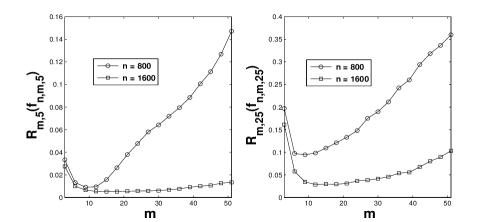
Figure 3: Performance of SVM forecasters for $l=5$ (left) and $l=25$ (right) steps ahead forecasts of the $x$ coordinate of the Lorenz dynamics with Gaussian noise with $\sigma=0.05$. The circles and squares report, as a function of the memory length $m$, the average risk of 25 SVM forecasters built from different samples of size $n=800$ and $n=1600$ for each $m$.

Let us now apply this nonparametric approach to predicting the evolution of the $x$-coordinate of the Lorenz system described by the following set of differential equations, $\dot{x}=a(y-x)$, $\dot{y}=bx-y-xz$, $\dot{z}=xy-cz$, where the parameters are set at the standard values $a=10$, $b=28$, and $c=8/3$. The evolution is sampled at time steps of $\tau=0.01$ and the observational error is i.i.d Gaussain noise. We compute SVM forecasters using memories of increasing length and for training data of two different sizes $n=800$ and $n=1600$. Since in estimating the convergence speed of (7) we are using a loose concentration result, a suitable regularization parameter and kernel width sequence cannot be chosen a-priori. Hence, we have adopted a grid search in $(\lambda,\gamma)$ space and a 4-fold cross-validation technique Györfi et al. (2002) to choose $(\lambda_{n},\gamma_{n})$ for a given sample size $n$. Finally, we use $(\lambda_{n},\gamma_{n})$ for an estimate $f_{n,1,1,\lambda_{n},\gamma_{n}}$ constructed from (6) using the whole sample $T_{n}$ (to simplify notation, we henceforward omit the dependence of $f_{n,1,1}$ on the regularization parameters $(\lambda_{n},\gamma_{n})$). This approach adapts the regularization parameters and the complexity of the SVM forecasters to the amount of available empirical data. The risk of each forecaster is estimated by the prediction error over a large test set ($10^{5}$ input/output pairs) chosen independent of the training set $T_{n}$. Note that ${{\cal R}_{m,l}(f)}\geq\sigma^{2}$, where $\sigma$ is the standard deviation of the noise.

As Fig. (3) shows for $l\in\{5,25\}$, by increasing the memory of the predictor we obtain forecasters with improved performance. However, for a given sample size $n$, there is an optimal memory length $m$ and increasing memory length beyond this value produces poorer forecaster due to their increased complexity for the available data. Moreover the memory of the best forecaster increases with sample size from $m\approx 9$ for $n=800$ to $m\approx 18$ for $n=1600$, as shown for $5$-step ahead forecasters, while the memory increases from $m\approx 9$ for $n=800$ to $m\approx 12$ for $n=1600$, for $25$-step ahead forecasters. This reflects the fact that with increased information we can build more complex and, therefore, better predictors. Since forecasting further into the future is a more difficult problem, the performance of the predictor decreases when we keep the same sample size but attempt to make $25$-steps ahead predictions. Furthermore, as the right plot in Fig. 3 reveals, for the same sample size $n$ the memory of the best forecaster reduces in order to accommodate the increased complexity of the learning task.

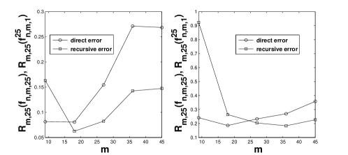
Figure 4: Performance of direct and recursive SVM forecasters for $l=25$ steps ahead forecasts of the $x$ coordinate of the Lorenz dynamics with Gaussian noise with $\sigma=0.20$ (left) and $\sigma=0.05$ (right). The circles and squares report, as a function of the memory length $m$, the averages forecasting risk of 30 direct and recursive SVM forecasters built from different samples of size $n=800$ for each $m$.

In the limit $n\rightarrow\infty$ direct forecasts are better than recursive forecasts because the SVM forecaster approaches the Bayes forecaster. However, for finite sample sizes this is not always the case. Indeed, as Fig. (4) shows for $n=800$ there is a memory size at which the risk of the direct forecaster, $f_{n,m,25}$, is larger than that of the recursive, $f_{n,m,1}^{25}$, $25$-steps ahead forecaster. Moreover, the crossover depends on the amount of noise and increases as noise variance increases while keeping the same sample size $n$. By increasing the sample size though, the crossover increases such that in the limit of infinite sample size direct forecasters always perform better than recursive forecasters, as is expected.

To conclude, we have described the assumptions under which non-parametric SVM forecasters can consistently learn the optimal predictors. For example, for bounded noise, SVM forecasters are consistent for all pairs of dynamical systems and observational noise processes that possess summable correlation sequences. Hence, the SVM forecasters possess a weak form of universality for a large class of stochastic processes. This includes systems with smooth uniformly expanding dynamics or smooth hyperbolic dynamics, systems perturbed by dynamic noise, as well as ”parabolic” or ”intermittent” systems which have a polynomial decay of correlations Baladi (2000). Remarkably, for some dynamical systems it seems possible to decide on the summability of the correlation sequence from observations. Indeed, for piecewise expanding maps rigorous estimates of the asymptotic rate of decay of correlations for a given function is numerically feasible Liverani (2001).

We also notice that in the presence of observational noise the task of forecasting is different from the task of modelling the underlying nonlinear dynamics from data. Indeed, finding the simplest model consistent with the observations, which is the ultimate goal of modelling Kantz and Schreiber (2004), is highly unsuitable for forecasting. This is clearly illustrated by noticing the significant increase of forecasting skill in Fig. (3) when using a memory length which is much larger than the minimal time delay embedding necessary to reconstruct a modelling phase space equivalent to the original state space of the Lorenz system.

Finally, we note that our analysis remains valid for stationary nonergodic processes. Since a nonergodic stationary process has an ergodic decomposition, a realization of the time series falls with probability one into an invariant event on which the process is ergodic and stationary. For this reason, the proposed learning algorithm can be applied to a time series sequence generated by that event as though it were the process universe.

References

- Maybeck (1979) P. S. Maybeck, Stochastic models, Estimation, and Control (Academic Press, Inc., 1979).
- Doucet et. al. (2000) A. Doucet et. al., Statistics and Computing 10, 197 (2000).
- Beck and Schlögl (1993) C. Beck and F. Schlögl, Thermodynamics of Chaotic Systems (Cambridge University Press, 1993).
- (4) In order to obtain the optimal denoiser we have to minimize a modified risk functional, i.e. which assumes, unrealistically, exact knowledge of the state, , that we want to estimate by denoising. Nevertheless, by carrying out the minimization we obtain Eq. (4) with , which is computationally feasible when perfect knowledge about the dynamics and the noise is assumed.
- Györfi et al. (2002) L. Györfi et al., A Distribution-free Theory of Nonparametric Regression (Springer, New York, 2002).
- Modha and Masry (1998) D. Modha and E. Masry, IEEE Transactions on Information Theory 44, 117 (1998).
- Meir (2000) R. Meir, Machine learning 39, 5 (2000).
- Schölkopf and Smola (2002) B. Schölkopf and A. Smola, Learning with Kernels (MIT Press, Cambridge, MA, 2002).
- Cucker and Smale (2002) F. Cucker and S. Smale, Bull. Amer. Math. Soc. 39, 1 (2002).
- Steinwart et al. (2006) I. Steinwart et al. (2006), arXiv:0707.0303, submitted to the J. Multivariate Anal.
- Nobel (1999) A. Nobel, Ann. Statist. 27, 262 (1999).
- Steinwart and Anghel (2007) I. Steinwart and M. Anghel (2007), arXiv:0707.0322, submitted to the Annals of Statistics.
- Baladi (2000) V. Baladi, Positive Transfer Operators and Decay of Correlations (World Scientific, 2000).
- Liverani (2001) C. Liverani, Nonlinearity 14, 463 (2001).
- Kantz and Schreiber (2004) H. Kantz and T. Schreiber, Nonlinear Time Series Analysis (Cambridge University Press, 2004), 2nd ed.