Effect of Holstein phonons on the electronic properties of graphene

Abstract

We obtain the self-energy of the electronic propagator due to the presence of Holstein polarons within the first Born approximation. This leads to a renormalization of the Fermi velocity of one percent. We further compute the optical conductivity of the system at the Dirac point and at finite doping within the Kubo-formula. We argue that the effects due to Holstein phonons are negligible and that the Boltzmann approach which does not include inter-band transition and can thus not treat optical phonons due to their high energy of $\hbar\omega_{0}\sim 0.1-0.2$eV, remains valid.

1 Introduction

Three years ago, Geim, Novoselov and co-workers have succeeded in isolating and contacting a single layer of graphite (graphene).[1] Contrary to common wisdom, this experiment showed that true two-dimensional lattices are thermodynamically stable. [2, 3] This stability comes about because the system gently crumples to the third direction forming ripples. [4] It is therefore an important problem to study the effect of out-plane phonons on the electronic properties of the system. Contrary to two-dimensional electron-systems in semiconductor heterostructures, where (scalar) electrons interact with bulk[5] or surface[6] phonons, in graphene there are two-dimensional in-plane as well as out-of-plane vibrational modes to which Dirac (spinor) fermions will couple.

There are two different vertex-types modeling the interaction of electrons with optical phonons. First, due to the atomic displacement within the plane, the tunneling-matrix element between two carbon atoms varies. This gives rise to a Su-Schrieffer-Heeger type coupling (current-current coupling).[7] The two-dimensional gauge field is composed by the longitudinal optical (LO) and transverse optical (TO) phonons which are degenerate at $q=0$. This vertex type is also found from symmetry arguments.[8] There are also out-of-plane vibrations. These lattice displacements are symmetric with respect to their neighboring atoms and thus couple to the electronic densities. The optical (ZO) modes can then be described within the Holstein model.[9] For a recent account on the Green’s function of the Holstein polaron, see Ref. [10] and references therein.

Out-of-plane modes are energetically smaller than in-plane vibrations due to the hybridization of the $sp^{2}$-orbitals within the graphene sheet. A tight-binding calculation including nearest and second-nearest neighbors yields $\omega_{\rm ZO}\approx\omega_{\rm LO}/2$ for the optical branch close to the $\Gamma$-point.[11] For a first-principle calculation of the phonon-spectra, see the work by Wirtz and Rubio.[12] The effect of the electron-phonon coupling on the local density of states of zig-zag graphene ribbons has been studied by Sasaki et al..[13] The effect of the optical phonons on the Raman spectrum of disordered graphene was studied by Castro Neto and Guinea. [14]

The effect of Holstein phonons on transport properties has been receiving renewed interest in the context of the one-dimensional Holstein-Hubbard model.[15] Here, we will discuss Holstein phonons in graphene for the following reason. It is currently believed that transport properties can be well described within a semi-classical Boltzmann approach.[16, 17, 18] This implies well-defined quasi-particles, i.e., only one band is considered and inter-band transitions are ruled out. Doing so, several scattering mechanisms have been discussed, ranging from local defects (vacancies or substitutions), long-ranged Coulomb impurities in the substrate or due to adsorbed atoms to acoustical phonons.[19, 20]

Optical phonons cannot be treated within the one-band Boltzmann approach[21] since they would induce interband-transitions at typical densities of $n\lower 3.50006pt\hbox{$\stackrel{{\scriptstyle\textstyle<}}{{\sim}}$}5\times 10^{12}$cm^-2. It is therefore crucial to assess this scattering mechanism via the Kubo-formalism. In section II, we present our model for Holstein phonons and calculate the electronic self-energy within the first Born approximation in section III. We further compute the optical conductivity in section IV, using the full Greens function, but neglecting vertex corrections. We close with conclusions and outlook.

2 The effective model

In two-dimensional graphene sheets, first-principle calculations reveal that the Born-Oppenheimer approximation is not valid for doped graphene sheets.[22] Fröhlich polarons[23] are thus not a good starting point to describe electron-lattice interaction in graphene. Here, we present the study of the electron-lattice coupling due to localized Holstein-phonons in a two-dimensional honeycomb lattice, thus treating the ZO-phonons (out-of-plane vibrations).

The honeycomb lattice (the lattice of graphene) is made of two interpenetrating triangular lattices, defining two non-equivalent sites, usually labeled as $A$ and $B$ sites.[24] The model Hamiltonian for ZO-polarons in graphene reads as follows:

$$H-t\sum_{i,\sigma\bm{\delta}}\left[a^{\dagger}_{\sigma}(\bm{R}_{i})b_{\sigma}(\bm{R}_{i}+\bm{\delta})+{\rm H.c.}\right]+\sum_{\bm{q}}\omega_{\bm{q}}c^{\dagger}_{\bm{q}}c_{\bm{q}}+V_{ep}$$ (1)

where $a^{\dagger}_{\sigma}(\bm{R}_{i})$ ($b^{\dagger}_{\sigma}(\bm{R}_{i})$) creates an electron at an atom of the $A$(B) sub-lattice and $c^{\dagger}_{\bm{q}}$ are creation phonon operators. The energy $\omega_{\bm{q}}$ is the dispersion of the ZO-phonon and $V_{ep}$ the electron-phonon interaction. We model the coupling to the ZO-phonons as the usually density-density coupling[25]

$$V_{ep}=D\sum_{\sigma,i,j}\left[a^{\dagger}_{\sigma}(\bm{R}_{i})a_{\sigma}(\bm{R}_{i})+b^{\dagger}_{\sigma}(\bm{R}_{i})b_{\sigma}(\bm{R}_{i})-1\right]Q_{j}\,,$$ (2)

with $Q_{j}$ defined as

$$Q_{j}=\sum_{\bm{q}}X_{\bm{q}}e^{i\bm{q}\cdot\bm{R}_{j}}(c_{\bm{q}}+c^{\dagger}_{-\bm{q}})\,,$$ (3)

and

$$X_{\bm{q}}=\sqrt{\frac{\hbar^{2}}{2MN\omega_{\bm{q}}}}$$ (4)

and $M$ the ion’s mass and $N$ the number of unit cells in the crystal. Note that we couple the density with respect to the half-filled band such that particle-hole symmetry is conserved by reversing the sign of the coupling constant. In the following, though, we shall neglect this shift in the bosonic operators.

The effect of Holstein polarons is obtained using $\omega_{\bm{q}}\simeq\omega_{0}$ and transforming the operators in Hamiltonian (1) to momentum space. This gives

$$H=-t\sum_{\bm{q},\sigma}\left(\phi_{\bm{q}}a^{\dagger}_{\bm{q},\sigma}b_{\bm{q},\sigma}+{\rm H.c.}\right)+\sum_{\bm{q}}\omega_{0}c^{\dagger}_{\bm{q}}c_{\bm{q}}+V_{ep}\,,$$ (5)

with $\phi_{\bm{q}}=\sum_{\bm{\delta}}e^{-i\bm{\delta}\cdot\bm{q}}$, $\bm{\delta}$ the vectors connecting the three nearest neighbors on the honeycomb lattice, and $V_{ep}$ given by

$$V_{ep}=D\sum_{\bm{p},\bm{q},\sigma}X_{\bm{q}}\left(a^{\dagger}_{\bm{p},\sigma}a_{\bm{p}+\bm{q},\sigma}+b^{\dagger}_{\bm{p},\sigma}b_{\bm{p}+\bm{q},\sigma}\right)\left(c_{\bm{q}}+c^{\dagger}_{-\bm{q}}\right)\;.$$ (6)

Let us comment on the coupling constant $D$. Due to the mirror symmetry of the graphene-sheet, one might think that the linear coupling to lattice displacements is zero. But the mirror symmetry is broken for samples where graphene lies on top of a SiO₂- or SiC-substrate (for a discussion, see Ref. [8]). To quantify the coupling constant in terms of the dimensionless constant $g=\sqrt{N}DX_{0}/\omega_{0}$, we assume that the coupling mechanism is due to a variation of the hopping matrix element. This yields $g$ of the order of unity.[14]

3 Second order perturbation theory

If the phonon energy scale is much smaller than the electronic energy scale, Migdal’s theorem states that it is sufficient to calculate the lowest-order self-energy diagram.[26] This diagram can further be calculated using the bare electron Greens function. Still, the importance of electron-phonon coupling also depends on the dimensionality of the system. E.g., in self-assembled quantum dots, vertex ”corrections” to the polarization of an electron-hole pair give rise to charge-cancellation,[27] thus changing the optical conductivity significantly.[28] Also for $A_{3}{\rm C}_{60}$ ($A$=K,Rb)[29] and for general one-dimensional systems,[30] Migdal’s theorem is not valid. Furthermore, electron-electron interaction can affect the effective electron-phonon interaction.[15]

In graphene sheets, electron-electron interaction is generally neglected, i.e., one assumes a “normal” ground-state at zero doping (one electron per unit cell) - characterized by a semi-metal. Since the average kinetic and interaction energy per particle both scale with $\sqrt{n}$ where $n$ is the carrier density, the interaction does not become important at finite doping, either. Electron-electron interaction is also neglected in recent works on localization[31] even though disorder enhances the effect of interaction.[32] The same should hold for the electron-phonon vertex corrections which results in an effective electron-electron interaction and we thus believe that the assumption of Migdal’s theory is a good starting point to discuss the Holstein-phonons in graphene.

Because of the existence of two sub-lattices, the Green’s function needs to be written as a $2\times 2$ matrix:

$$\bm{G}_{\sigma}(\bm{k},\tau)=\left(\begin{array}[]{cc}G_{AA,\sigma}(\bm{k},\tau)&G_{AB,\sigma}(\bm{k},\tau)\\ G_{BA,\sigma}(\bm{k},\tau)&G_{BB,\sigma}(\bm{k},\tau)\end{array}\right)\,,$$ (9)

with

$$G_{AA,\sigma}(\bm{k},\tau) = -\langle{\cal T}a_{\bm{k},\sigma}(\tau)a_{\bm{k},\sigma}^{{\dagger}}(0)\rangle\,,$$

$$G_{AB,\sigma}(\bm{k},\tau) = -\langle{\cal T}a_{\bm{k},\sigma}(\tau)b_{\bm{k},\sigma}^{{\dagger}}(0)\rangle\,,$$

$$G_{BA,\sigma}(\bm{k},\tau) = -\langle{\cal T}b_{\bm{k},\sigma}(\tau)a_{\bm{k},\sigma}^{{\dagger}}(0)\rangle\,,$$

$$G_{BB,\sigma}(\bm{k},\tau) = -\langle{\cal T}b_{\bm{k},\sigma}(\tau)b_{\bm{k},\sigma}^{{\dagger}}(0)\rangle\,,$$ (10)

where $\tau$ is the “imaginary” time, and ${\cal T}$ is the time ordering operator.

Up to second order in perturbation theory, and after transforming the time dependence of the Green’s function to Matsubara frequencies, we obtain the following result:

$${\bm{G}}={\bm{G}^{(0)}}+{\bm{G}^{(0)}}{\bm{\Sigma}}{\bm{G}^{(0)}}\,,$$ (11)

where the matrix ${\bm{\Sigma}}$ is defined as

$$\bm{\Sigma}=\left(\begin{array}[]{cc}\Sigma_{AA}&\Sigma_{AB}\\ \Sigma_{BA}&\Sigma_{BB}\end{array}\right)\,,$$ (12)

and the matrix element $\Sigma_{\alpha\beta}$ is defined by ($\alpha,\beta=A,B$)

$$\Sigma_{\alpha\beta}(i\omega_{n},\bm{p})=-\frac{1}{\beta}\sum_{\bm{q},\nu}D^{2}X^{2}_{\bm{q}}D^{(0)}(\bm{q},i\nu)G^{(0)}_{\alpha\beta}(\bm{p}-\bm{q},i\omega_{n}-i\nu).$$ (13)

Because both $X_{\bm{q}}$ and $D^{(0)}(\bm{q},i\nu)$ are momentum independent, i.e., we set $\omega_{\bm{q}}=\omega_{0}$ and the phonon propagator $D^{(0)}(\bm{q},i\nu)$ is given by

$$D^{(0)}(\bm{q},i\nu)=\frac{2\omega_{0}}{(i\nu)^{2}-\omega^{2}_{0}}\,,$$ (14)

the matrix elements of the self energy matrix can be written in a simplified form, reading $\Sigma_{\alpha\beta}(i\omega_{n})=-\frac{1}{\beta}\sum_{\bm{q},\nu}D^{2}X^{2}_{0}D^{(0)}(i\nu)G^{(0)}_{\alpha\beta}(\bm{q},i\omega_{n}+i\nu)\;$ where $X_{0}$ is $X_{\bm{q}}$ with $\omega_{\bm{q}}$ replaced by $\omega_{0}$. Notice that we neglected the constant shift in the self-energy due to the shift of the bosonic displacement operator, still present in Eq. (13). This is consistent since we also neglected the Hartree correction to the self energy.

From the above we can write down a Dyson equation for the electronic propagator, given by

$${\bm{G}}={\bm{G}^{(0)}}+{\bm{G}^{(0)}}{\bm{\Sigma}}{\bm{G}}\,,$$ (15)

which has to be solved for ${\bm{G}}$. The equation giving the Matsubara Green’s function for the free electronic system reads

$$\left(\begin{array}[]{cc}i\omega_{n}&-t\phi(\bm{k})\\ -t\phi^{\ast}(\bm{k})&i\omega_{n}\end{array}\right){\bm{G}^{(0)}(i\omega_{n},\bm{k})}={\bm{1}}\,,$$ (16)

and ${\bm{1}}$ is the $2\times 2$ unit matrix. Within the Dirac cone approximation, which applies in a range of 1 eV, one has $\Sigma_{AB}(i\omega_{n})=\Sigma_{BA}(i\omega_{n})=0$. Also the following result holds $\Sigma_{AA}(i\omega_{n})=\Sigma_{BB}(i\omega_{n})=\Sigma(i\omega_{n})$ leading to a simplified form for the Dyson equation (15), which can be readily solved, giving

$${\bm{G}}=\frac{\left(\begin{array}[]{cc}i\omega_{n}-\Sigma(i\omega_{n})&t\phi(\bm{k})\\ t\phi^{\ast}(\bm{k})&i\omega_{n}-\Sigma(i\omega_{n})\end{array}\right)}{(i\omega_{n}-\Sigma)(i\omega_{n}-\Sigma)-t^{2}|\phi|^{2}}\;.$$ (17)

The matrix elements of Eq. (17) can be put into a simpler form reading

$${G}_{AA}(\omega_{n},{\bm{k}}) = \sum_{j=\pm 1}\frac{1/2}{i\omega_{n}-\Sigma(i\omega_{n})-jt|\phi(\bm{k})|}\,,$$ (18)

$${G}_{AB}(\omega_{n},{\bm{k}}) = \sum_{j=\pm 1}\frac{je^{i\delta(\bm{k})}/2}{i\omega_{n}-\Sigma(i\omega_{n})-jt|\phi(\bm{k})|}\,,$$ (19)

$${G}_{BA}(\omega_{n},\bm{k}) = \sum_{j=\pm 1}\frac{je^{-i\delta(\bm{k})}/2}{i\omega_{n}-\Sigma(i\omega_{n})-jt|\phi(\bm{k})|}\,,$$ (20)

$${G}_{BB}(\omega_{n},{\bm{k}}) = {G}_{AA}(\omega_{n},\bm{k})\,.$$ (21)

The summation over the bosonic frequency $\nu$ in Eq. (3) can be performed using standard methods leading to

$$\Sigma(i\omega_{n})=\sum_{\bm{q},j=\pm 1}D^{2}X^{2}_{0}\frac{1}{2}\left(\frac{N_{0}+n_{F}(jt|\phi(\bm{q})|)}{i\omega_{n}-jt|\phi(\bm{q})|+\omega_{0}}+\frac{N_{0}+1-n_{F}(jt|\phi(\bm{q})|)}{i\omega_{n}-jt|\phi(\bm{q})|-\omega_{0}}\right)\,.$$ (22)

The integrals over the momentum variable in Eq. (22) can be easily computed at zero temperature and within the Dirac cone approximation, yielding an explicit form for the self energy.

3.1 Zero doping

At zero temperature and zero chemical potential (that is at the neutrality point) the self energy, denoted by $\Sigma\rightarrow\Sigma_{0}$, has a simplified form reading

$$\Sigma_{0}(i\omega_{n})=\frac{g^{2}\omega^{2}_{0}}{N\hbar^{2}}\sum_{\bm{q}}\frac{1}{2}\left(\frac{1}{i\omega_{n}-t|\phi(\bm{q})|/\hbar-\omega_{0}/\hbar}+\frac{1}{i\omega_{n}+t|\phi(\bm{q})|/\hbar+\omega_{0}/\hbar}\right)$$ (23)

where we have introduced the missing $\hbar$’s omitted in the beginning of this section and $g$ denotes a dimensionless coupling constant of order unity, defined below Eq. (6). Performing the analytical continuation $i\omega_{n}\rightarrow\omega+i\delta$ and computing the momentum integral in Eq. (23) one obtains the retarded self energy, $\Sigma^{\rm ret}(\omega)$, of the polaron problem, which reads

$$\Sigma_{0}^{\rm ret}(\omega)=\frac{A_{c}}{2\pi}\left(\frac{g\omega_{0}}{\hbar}\right)^{2}\left(-\frac{\omega}{v^{2}_{F}}\ln\left|\frac{(v_{F}k_{c})^{2}}{\omega^{2}-(\omega_{0}/\hbar)^{2}}\right|\right.$$

$$+ \left.\frac{\omega_{0}/\hbar}{v_{F}^{2}}\ln\left|\frac{\omega+\omega_{0}/\hbar}{\omega-\omega_{0}/\hbar}\right|\right)-i\pi\frac{A_{c}}{2\pi}\left(\frac{g\omega_{0}}{\hbar}\right)^{2}$$

$$\times \left[\left(\frac{\omega}{v^{2}_{F}}-\frac{\omega_{0}}{v^{2}_{F}\hbar}\right)\theta(\omega-\omega_{0}/\hbar)\theta(v_{F}k_{c}+\omega_{0}/\hbar-\omega)\right.$$

$$- \left.\left(\frac{\omega}{v^{2}_{F}}+\frac{\omega_{0}}{v^{2}_{F}\hbar}\right)\theta(-\omega-\omega_{0}/\hbar)\theta(v_{F}k_{c}+\omega_{0}/\hbar+\omega)\right]\,,$$

with $\pi k_{c}^{2}=(2\pi)^{2}/A_{c}$, $A_{c}=a^{2}3\sqrt{3}/2$, and $a=1.42$ Å.

One can easily obtain the renormalization of the electronic spectrum due to the retarded self-energy induced by the phonons, using Rayleigh-Schrödinger perturbation theory.[25] In this scheme, the $\omega$ dependence of the self-energy is replace by the bare electronic dispersion. Close to the Dirac point, the dispersion is simply given by $\omega=\pm v_{F}k$ where the upper (lower) sign holds for electrons (holes) and we obtain the new energy spectrum $E(\bm{k})$ from

$$E(\bm{k})=v_{F}\hbar k+\hbar\Re\Sigma_{0}^{\rm ret}(v_{F}k)\,$$ (25)

for the conduction band and

$$E(\bm{k})=-v_{F}\hbar k+\hbar\Re\Sigma_{0}^{\rm ret}(-v_{F}k)\,$$ (26)

for the valence band. Electron-hole symmetry is thus preserved, if $\Re\Sigma_{0}^{\rm ret}(x)=-\Re\Sigma_{0}^{\rm ret}(-x)$ which is the case (see Eq. (3.1)).

Considering that $v_{F}k$ is the smallest energy in the problem, that is $k$ is very close to the Dirac point, we obtain for $\Re\Sigma_{0}^{\rm ret}(v_{F}k)$ the result

$$\Re\Sigma_{0}^{\rm ret}(v_{F}k)=-v_{F}k\frac{A_{c}}{\pi v_{F}^{2}}\left(\frac{g\omega_{0}}{\hbar}\right)^{2}\ln\frac{v_{F}k_{c}}{\omega_{0}/\hbar}\,.$$ (27)

Considering the out-of-plane optical mode of graphene[12], which has an energy of $\omega_{ZO}\simeq 0.1$ eV and using $g^{2}=10$ we obtain

$$\frac{A_{c}}{\pi v_{F}^{2}}\left(\frac{g\omega_{0}}{\hbar}\right)^{2}\ln\frac{v_{F}k_{c}}{\omega_{0}/\hbar}\simeq 0.02\;.$$ (28)

In Fig. 1, the renormalized energy dispersion is shown for various values of the coupling constant. We also included a large coupling constant $g=10$ for better illustration of the effect of the electron-phonon interaction.

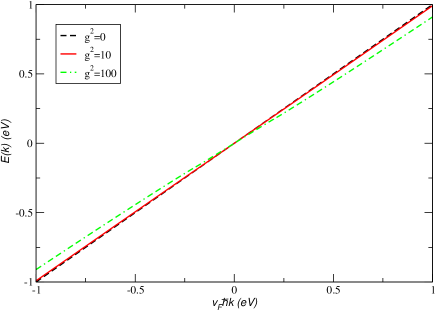
Figure 1: (Color online) Renormalized energy band at the neutrality point, given by $E(\bm{k})=\pm v_{F}\hbar k\pm\hbar\Re\Sigma_{0}^{\rm ret}(v_{F}k)$ for two different values of the coupling constant $g$.

3.2 Finite doping

At finite doping, the one-particle dispersion $j|\phi(\bm{k})|$ must be replaced by $j|\phi(\bm{k})|-\mu$ in Eqs. (18) - (21) and Eq. (22), where $\mu=\hbar v_{F}k_{F}$ denotes the Fermi energy. The retarded self-energy can then be written as $\Sigma_{\mu}^{\rm ret}(\omega)=\Sigma_{0}^{\rm ret}(\omega+\mu/\hbar)+\Delta\Sigma(\omega+\mu/\hbar)$ where we have

$$\Delta\Sigma(\omega)=\frac{A_{c}}{2\pi}\left(\frac{g\omega_{0}}{\hbar}\right)^{2}\left(-\frac{\omega_{0}/\hbar}{v_{F}^{2}}\ln\left|\frac{(\mu/\hbar-\omega)^{2}-(\omega_{0}/\hbar)^{2}}{\omega^{2}-(\omega_{0}/\hbar)^{2}}\right|\right.$$

$$\left.-\frac{\omega}{v_{F}^{2}}\ln\left|\frac{(\mu/\hbar-\omega-\omega_{0}/\hbar)(\omega-\omega_{0}/\hbar)}{(\mu/\hbar-\omega+\omega_{0}/\hbar)(\omega+\omega_{0}/\hbar)}\right|\right)-$$

$$i\pi\frac{A_{c}}{2\pi}\left(\frac{g\omega_{0}}{\hbar}\right)^{2}\left[\left(\frac{\omega}{v^{2}_{F}}+\frac{\omega_{0}}{v^{2}_{F}\hbar}\right)\theta(\omega+\omega_{0}/\hbar)\theta(\mu/\hbar-\omega_{0}/\hbar-\omega)\right.$$

$$\left.-\left(\frac{\omega}{v^{2}_{F}}-\frac{\omega_{0}}{v^{2}_{F}\hbar}\right)\theta(\omega-\omega_{0}/\hbar)\theta(\mu/\hbar+\omega_{0}/\hbar-\omega)\right]\,.$$ (29)

We note that for finite doping $\Sigma_{\mu}^{\rm ret}(\omega)$ diverges logarithmically at $\omega=\pm\omega_{0}/\hbar$.

4 Optical conductivity

In this section we want to compute the optical conductivity of graphene and study how the conductivity of the system is affected by the out-of-plane (ZO) phonons. To determine the conductivity one needs to know the current operator $j_{x}$, which is composed of the paramagnetic and diamagnetic contributions $j_{x}=j_{x}^{P}+A_{x}(t)j_{x}^{D}$, each of them given by[33]

$$j^{P}_{x}=-\frac{itea}{2\hbar}\sum_{\bm{k},\sigma}\left[(\phi(\bm{k})-3)a_{\sigma}^{\dagger}(\bm{k})b_{\sigma}(\bm{k})-(\phi^{\ast}(\bm{k})-3)b^{\dagger}_{\sigma}(\bm{k})a_{\sigma}(\bm{k})\right]\,,$$ (30)

and

$$j^{D}_{x}=-\frac{te^{2}a^{2}}{4\hbar^{2}}\sum_{\bm{k},\sigma}\left[(\phi(\bm{k})+3)a_{\sigma}^{\dagger}(\bm{k})b_{\sigma}(\bm{k})+(\phi^{\ast}(\bm{k})+3)b^{\dagger}_{\sigma}(\bm{k})a_{\sigma}(\bm{k})\right]\,.$$ (31)

The Kubo formula for the conductivity is given by[34]

$$\sigma_{xx}(\omega)=\frac{<j^{D}_{x}>}{iA_{s}(\omega+i0^{+})}+\frac{\Lambda_{xx}(\omega+i0^{+})}{i\hbar A_{s}(\omega+i0^{+})}\,,$$ (32)

with $A_{s}=N_{c}A_{c}$ the area of the sample, and $A_{c}$ the area of the unit cell, from which it follows that

$$\Re\sigma(\omega)=D\delta(\omega)+\frac{\Im\Lambda_{xx}(\omega+i0^{+})}{\hbar\omega A_{s}}\,,$$ (33)

where $D$ is the charge stiffness which reads

$$D=-\pi\frac{<j^{D}_{x}>}{A_{s}}-\pi\frac{\Re\Lambda_{xx}(\omega+i0^{+})}{\hbar A_{s}}\,.$$ (34)

The incoherent contribution to the conductivity $\Lambda_{xx}(\omega+i0^{+})$ is obtained from $\Lambda_{xx}(i\omega_{n})$, with this latter quantity defined as

$$\Lambda_{xx}(i\omega_{n})=\int_{0}^{\beta}d\,\tau e^{i\omega_{n}\tau}<T_{\tau}j^{P}_{x}(\tau)j^{P}_{x}(0)>\,.$$ (35)

The relevant quantity $\Im\Lambda_{xx}(\omega+i0^{+})$ is given by

$$\Im\Lambda_{xx}(\omega+i0^{+})=\frac{t^{2}e^{2}a^{2}}{16\hbar^{2}}\int\frac{d\,\epsilon}{2\pi\hbar}\sum_{\bm{k}}\sum_{\lambda_{1},\lambda_{2}=\pm 1}$$

$$\left[n_{F}(\epsilon)-n_{F}(\epsilon+\omega\hbar)\right]A^{\lambda_{1}}(\bm{k},\omega+\epsilon/\hbar)A^{\lambda_{2}}(\bm{k},\epsilon/\hbar)f(\bm{k},\lambda_{1},\lambda_{2})\,,$$ (36)

with $A^{\lambda}(\bm{k},\omega)$ given by

$$A^{\lambda}(\bm{k},\omega)=-2\Im G^{\lambda}_{R}(\bm{k},\omega+i0^{+})\,,$$ (37)

$G^{\lambda}(\bm{k},i\omega)$ given by

$$G^{\lambda}(\bm{k},i\omega_{n})=\frac{1}{i\omega_{n}-\Sigma(i\omega_{n})-(\lambda t|\phi(\bm{k})|-\mu)/\hbar}\,,$$ (38)

and $f(\bm{k},\lambda_{1},\lambda_{2})$ given by

$$f(\bm{k},\lambda_{1},\lambda_{2})=2|\phi(\bm{k})-3|^{2}-\lambda_{1}\lambda_{2}\left[(\phi^{\ast}(\bm{k})-3)^{2}\frac{\phi^{2}(\bm{k})}{|\phi(\bm{k})|^{2}}+(\phi(\bm{k})-3)^{2}\frac{(\phi^{\ast}(\bm{k}))^{2}}{|\phi(\bm{k})|^{2}}\right].$$ (39)

Using the fact that

$$\sum_{\bm{k}}\phi(\bm{k})g(|\phi(\bm{k})|)=\sum_{\bm{k}}\phi^{\ast}(\bm{k})g(|\phi(\bm{k})|)=\frac{1}{3}\sum_{\bm{k}}|\phi(\bm{k})|^{2}g(|\phi(\bm{k})|)$$ (40)

where $g(|\phi(\bm{k})|)$ is an arbitrary function of the absolute value of $\phi(\bm{k})$, and the fact that in the Dirac cone approximation one has

$$\frac{\phi^{2}(\bm{k})}{|\phi(\bm{k})|^{2}}\simeq e^{i2\pi/3}[\cos(2\theta)-i\sin(2\theta)]\,,$$ (41)

and a similar expression for the complex conjugate expression $[\phi^{\ast}(\bm{k})]^{2}/|\phi(\bm{k})|^{2}$, one obtains a simplified expression for (36), given by

Figure 2: (Color online) Optical conductivity for two different values of the coupling constant $g$ at zero doping ($T=\Gamma=10^{-4}$eV). Inset: The relative conductivity $\Delta\sigma=\sigma(g=10)-\sigma(g=0)$ with and without $\Re\Sigma(\omega)$.

$$\Im\Lambda_{xx}(\omega+i0^{+})=\frac{t^{2}e^{2}a^{2}}{16\hbar^{2}}\int\frac{d\,\epsilon}{2\pi\hbar}\sum_{\bm{k}}\sum_{\lambda_{1},\lambda_{2}=\pm 1}$$

$$\left[n_{F}(\epsilon)-n_{F}(\epsilon+\omega\hbar)\right]A^{\lambda_{1}}(\bm{k},\omega+\epsilon/\hbar)A^{\lambda_{2}}(\bm{k},\epsilon/\hbar)$$

$$[18-2|\phi(\bm{k})|^{2}(\lambda_{1}\lambda_{2}+1)]\,.$$ (42)

The expression (42) is valid only in the Dirac cone approximation, and therefore one must replace $t|\phi(\bm{k})|$ by $v_{F}\hbar k$ and the integral over the momentum can be easily done. If one ignores the effect of phonons the calculation is straightforward, leading to a conductivity of the form (at zero doping)[33]

$$\Re\sigma(\omega)=\frac{\pi}{2}\frac{e^{2}}{h}\left(1-\frac{(\hbar\omega)^{2}}{18t^{2}}\right)\tanh\left(\frac{\omega\hbar}{4k_{B}T}\right)\,.$$ (43)

One should note that from Eq. (43) one has $\Re\sigma(0)=0$ for finite $T$. This is not seen in Fig. 2 because the temperature scale is very small.

The solution of Eq. (42) allows us to determine the optical conductivity taking into account the effect of Holstein phonons. In addition, we mimic the effect of impurities by adding a small imaginary part $\Gamma$ to the self-energy

$$\Im\Sigma(\omega)=\Im\Sigma_{ep}(\omega)-\Gamma\,,$$ (44)

where $\Im\Sigma_{ep}(\omega)$ is obtained from Eq. (3.1).

There are two types of momentum integrals in (42), which have the form

$$I_{n}(\epsilon/\hbar,\omega,\lambda_{1},\lambda_{2})=\int^{k_{c}}_{0}dk\frac{k^{2n+1}}{[(A-\lambda_{1}k)^{2}+B^{2}][(C-\lambda_{2}k)^{2}+D^{2}]}\,,$$ (45)

with $n=0,1$. The analytical expressions are given in the appendix. The final energy integration can be done numerically.

In Fig. 2, the conductivity is shown for various coupling constants $g$ at zero doping and low temperature $T$ and damping $\Gamma$ due to impurity scattering. There is a drop of the conductivity (relative to the conductivity of a clean system) starting at around the phonon energy $\omega_{0}$ and reaching a constant value for $\omega\lower 3.50006pt\hbox{$\stackrel{{\scriptstyle\textstyle>}}{{\sim}}$}2\omega_{0}$. Without the real part of the electronic self-energy, there is a pronounced peak at twice the phonon energy. This is shown in the inset of Fig. 2, where we plot $\Delta\sigma=\sigma(g=10)-\sigma(g=0)$ for $T=\Gamma=0.0001$eV and including, respectively, not including $\Re\Sigma(\omega)$ in the above expressions. It is thus crucial to include the full self energy in the renormalization of the particle Green’s function.

We thus obtain as main result that there remains no pronounced structure in the conductivity due to ZO-phonons if the full self-energy is used. We attribute this fact to the apparently asymmetric way the self-energy enters in the Green’s function with respect to the electron (j=1) and hole (j=-1) channel which destroys possible interferences between the two carriers (see Eq. (3.1)).

In Figs. 3 and 4, the optical conductivity is shown for different values of the coupling constant $g$ at $\mu=0.05$eV and $\mu=0.1$eV, respectively. The insets show the relative conductivity due to the electron-phonon interaction, $\Delta\sigma=\sigma(g=10)-\sigma(g=0)$, including, respectively, not including $\Re\Sigma(\omega)$ in the above expressions. Again we see a distinct difference in the result due to the renormalization of the electron-hole spectra.

It is clear that the results at finite chemical potential are markedly different from the results at the neutrality point. At finite chemical potential the system is characterized by a Drude like behavior followed by a strong increase of the conductivity when the photon frequency reach the value of twice the chemical potential. At zero doping there is no Drude weight and the system response is characterized only by inter-band transitions. We see only weak renormalization of the Drude peak due to the Holstein phonons as well as negligible effects at finite frequencies. We note that the results for $\Re\sigma(\omega)$ when $g=0$ were first obtained by Peres et al.[24] and by Gusynin et al..[35]

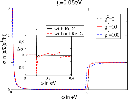
Figure 3: (Color online) Optical conductivity for two different values of the coupling constant $g$ at $\mu=0.05$eV ($T=\Gamma=10^{-4}$eV. Inset: The relative conductivity $\Delta\sigma=\sigma(g=10)-\sigma(g=0)$ with and without $\Re\Sigma(\omega)$.

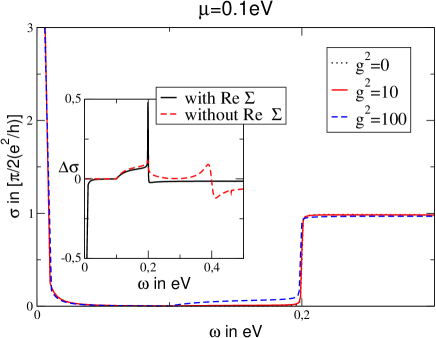
Figure 4: (Color online) Optical conductivity for two different values of the coupling constant $g$ at $\mu=0.1$eV ($T=\Gamma=10^{-4}$eV. Inset: The relative conductivity $\Delta\sigma=\sigma(g=10)-\sigma(g=0)$ with and without $\Re\Sigma(\omega)$.

5 Summary

In this paper, we have calculated the effect of Holstein polarons on the electronic properties of graphene. Holstein polarons arise through the coupling of out-of-plane optical (ZO) modes to the conduction electrons, described as Dirac Fermions. Throughout this work, we assumed Migdal’s theorem to be valid and calculated the electronic self-energy within the first Born approximation. We find that the Fermi velocity becomes renormalized within 1 %.

The main purpose of this work was to assess the effect of Holstein phonons on the conductivity within the Kubo-formula. Due to the large phonon-energy, electron scattering from Holstein phonons induces interband transitions for usual carrier densities (corresponding to a gate voltage of $\sim 50$V) and can thus not be treating within the one-band Boltzmann approach. We thus calculated the optical conductivity within the Kubo-formula, employing the full Green’s function but neglecting vertex corrections. We find a pronounced kink-like peak at twice the ZO-phonon energy if only the imaginary part of the self-energy is considered. This peak vanishes when the real part of the self-energy is included. Further, we see only weak renormalization of the Drude peak due to the Holstein phonons as well as negligible effects at finite frequencies. We conclude that scattering from Holstein-phonons can be neglected in usual transport properties.

The effect of lattice vibrations on the electronic properties of graphene is still not fully understood. Especially the coupling of substrate phonons[36] or in-plane oscillations to the conduction electrons is interesting. In the later case, this will lead to a non-diagonal electronic self-energy due to the current-current coupling.

Appendix A Momentum integrals

The momentum integrals have the form ($n=0,1$)

$$I_{n}=\int\frac{k^{2n+1}dk}{[(A-k)^{2}+B^{2}][(C-k)^{2}+D^{2}]}\;.$$ (46)

The general solution yields

$$I_{n} = \frac{-1}{G}\Big{[}F_{1}^{n}\tan^{-1}\left(\frac{A-k}{B}\right)+F_{2}^{n}\tan^{-1}\left(\frac{C-k}{D}\right)$$ (47)

$$- F_{3}^{n}\ln\left((A-k)^{2}+B^{2}\right)-F_{4}^{n}\ln\left((C-k)^{2}+D^{2}\right)\Big{]}$$

where the denominator reads $G=(B^{2}+(A-C)^{2})^{2}+2((A-C)^{2}-B^{2})D^{2}+D^{4}$ and the factors are given by

$$F_{1}^{0} = 4D(A^{3}-2A^{2}C-2B^{2}C+A(B^{2}+C^{2}+D^{2}))\;,$$

$$F_{2}^{0} = 4B((B^{2}+(A-C)^{2})C+(-2A+C)D^{2})\;,$$

$$F_{3}^{0} = -F_{4}^{0}=2BD(-A^{2}-B^{2}+C^{2}+D^{2})$$

and

$$F_{1}^{1} = 4D(A^{5}-2A^{4}C+2B^{4}C+A^{3}(2B^{2}+C^{2}+D^{2})+AB^{2}(B^{2}-3(C^{2}+D^{2})))\;,$$

$$F_{2}^{1} = 4B((B^{2}+(A-C)^{2})C^{3}+C(-3(A^{2}+B^{2})+2C^{2})D^{2}+(2A+C)D^{4})\;,$$

$$F_{3}^{1} = 2BD(A^{4}-4A^{3}C-4AB^{2}C+B^{2}(B^{2}-C^{2}-D^{2})+A^{2}(2B^{2}+3(C^{2}+D^{2})))\;,$$

$$F_{4}^{1} = 2BD(C^{2}(3(A^{2}+B^{2})-4AC+C^{2})-(A^{2}+B^{2}+4AC-2C^{2})D^{2}+D^{4})\;.$$

References

References

- [1] K. S. Novoselov, A. K. Geim, S. V. Morozov, D. Jiang, Y. Zhang, S. V. Dubonos, I. V. Grigorieva, and A. A. Firsov, Science 306, 666 (2004).
- [2] A. K. Geim and K. S. Novoselov, Nature Materials 6, 183 (2007).
- [3] G. E. Stein, E. J. Kramer, X. Li, and J. Wang, Phys. Rev. Lett. 98, 086101, (2007).
- [4] J. C. Meyer, A. K. Geim, M. I. Katsnelson, K. S. Novoselov, T. J. Booth, and S. Roth, Nature 446, 60 (2007).
- [5] W. Xiaoguang, F. M. Peeters, J. T. Devreese, Phys. Rev. B 31, 3420 (1985); S. Das Sarma and B. A. Mason, Ann. Phys. (N.Y.) 163, 78 (1985).
- [6] A. K. Sood, J. Menéndez, M. Cardona, and K. Ploog, Phys. Rev. Lett. 54, 2111 (1985); C. Trallero-Giner, F. García-Moliner, V. R. Velasco, and M. Cardona, Phys. Rev. B 45, 11944 (1992); A. J. Shields, M. Cardona, and K. Eberl, Phys. Rev. Lett. 72, 412 (1994).
- [7] W. P. Su, J. R. Schrieffer, and A. J. Heeger, Phys. Rev. Lett. 42, 1698 (1979).
- [8] J. L. Mañes, Phys. Rev. B 76, 045430 (2007).
- [9] T. Holstein, Ann. Phys. (N.Y.) 8, 325 (1959); 8, 343 (1959).
- [10] G. L. Goodvin, M. Berciu, and G. A. Sawatzky, Phys. Rev. B 74, 245104 (2006).
- [11] L. A. Falkovsky, cond-mat/0702409.
- [12] L. Wirtz and A. Rubio, Solid State Comm. 131, 141 (2004).
- [13] K. Sasaki, K. Sato, J. Jiang, R. Saito, S. Onari, and Y. Tanaka, Phys. Rev. B 75, 235430 (2007).
- [14] A. H. Castro Neto and F. Guinea, Phys. Rev. B 75, 045404 (2007).
- [15] A. Alvermann, D. M. Edwards, and H. Fehske, Phys. Rev. Lett. 98, 056602 (2007).
- [16] K. Nomura and A. H. MacDonald, Phys. Rev. Lett. 96, 256602 (2006).
- [17] S. Adam, E. H. Hwang, V. M. Galitski, and S. Das Sarma, Proc. Natl. Acad. Sci. USA 104, 18392 (2007).
- [18] N. M. R. Peres, J. M. B. Lopes dos Santos, and T. Stauber, Phys. Rev. B 76, 073412 (2007).
- [19] T. Stauber, N. M. R. Peres, and F. Guinea, Phys. Rev. B 76, 205423 (2007).
- [20] E. H. Hwang, S. Adam, S. Das Sarma, and A. K. Geim, Phys. Rev. B 76, 195421 (2007).
- [21] For a two-band formulation of the Botzmann equation, see M. Auslender and M. I. Katsnelson, arXiv:0707.2804.
- [22] M. Lazzeri and F. Mauri, Phys. Rev. Lett 97, 266407 (2006).
- [23] H. Fröhlich, Adv. Phys. 3, 325 (1954).
- [24] N. M. R. Peres, F. Guinea,and A. H. Castro Neto, Phys. Rev. B 73, 125411 (2006).
- [25] G. D. Mahan, Many-Particle Physics, (Kluwer/Plenum, 3ed).
- [26] A. B. Migdal, Zh. Eksp. Teor. Fiz. 34, 1438 (1958) [Sov. Phys. JETP 7, 996 (1958)].
- [27] S. Schmitt-Rink, D. A. B. Miller, and D. S. Chemla, Phys. Rev. B 35, 8113 (1987).
- [28] T. Stauber and R. Zimmermann, Phys. Rev. B 73, 115303 (2006).
- [29] O. Gunnarsson, V. Meden, and K. Schönhammer, Phys. Rev. B 50, 10462 (1994).
- [30] V. Meden, K. Schönhammer, and O. Gunnarsson, Phys. Rev. B 50, 11179 (1994).
- [31] I. L. Aleiner and K. B. Efetov, Phys. Rev. Lett. 97, 236801 (2006).
- [32] T. Stauber, F. Guinea, and M. A. H. Vozmediano, Phys. Rev. B 71, 041406(R) (2005).
- [33] N. M. R. Peres and T. Stauber, Int. J. Mod. Phys. B (in press), arXiv:0801.1625.
- [34] I. Paul and G. Kotliar, Phys. Rev. B 67, 115131 (2003).
- [35] V. P. Gusynin, S. G. Sharapov, and J. P. Carbotte, Phys. Rev. Lett. 96, 256802 (2006).
- [36] S. Fratini and F. Guinea, arXiv:0711.1303 (unpublished).