Embedded Rank Distance Codes for ISI channels

Abstract

Designs for transmit alphabet constrained space-time codes naturally lead to questions about the design of rank distance codes. Recently, diversity embedded multi-level space-time codes for flat fading channels have been designed from sets of binary matrices with rank distance guarantees over the binary field by mapping them onto QAM and PSK constellations. In this paper we demonstrate that diversity embedded space-time codes for fading Inter-Symbol Interference (ISI) channels can be designed with provable rank distance guarantees. As a corollary we obtain an asymptotic characterization of the fixed transmit alphabet rate-diversity trade-off for multiple antenna fading ISI channels. The key idea is to construct and analyze properties of binary matrices with a particular structure induced by ISI channels.

1 Introduction

Over the past decade significant progress has been made in constructing space-time codes that achieve the optimal rate-diversity trade-off for flat-fading channels when there are transmit alphabet constraints [18, 15]. Far less attention has been given to space-time code design and analysis for fading channels with memory, i.e., Inter-Symbol Interference (ISI) channels which are encountered in broadband multiple antenna communications. There have been several constructions of space-time codes for fading ISI channels using multi-carrier techniques (see for example [17] and references therein). However, since these inherently increase the transmit alphabet size, and the right framework to study such constructions is through the diversity-multiplexing trade-off [19]. We examined diversity embedded codes for ISI channels in [7], by considering the diversity-multiplexing trade-off.

As in space-time code design for flat-fading channels, it is natural to ask for a characterization of the rate-diversity trade-off for ISI channels with transmit alphabet constraints. The problem of constructing space-time codes with fixed transmit alphabet constraints is partially motivated by the need to control the transmit spectrum as well as the peak-to-average (PAR) ratio of the transmitted signal. For example, if we restrict transmission to PSK alphabet, it is clear that we have a unit peak-to-average ratio (PAR) making it possible to use efficient non-linear amplifiers (requiring small PAR), which are more efficient and hence suitable for mobile devices. Another important reason to consider this problem is a fundamental theoretical question, which is motivated by the origins of space-time codes for flat-fading channels in [18] where the constructions were for fixed transmit alphabet. For this constraint, there exists a trade-off between rate and diversity, for the flat-fading case. In this paper we ask the corresponding question for fading ISI channels. Since space-time code design with diversity order guarantees requires control over the rank distance of the codewords [18], the main topic of this paper is to design codes with rank distance guarantees for ISI channels.

Diversity embedded codes were introduced in [2] which allowed different parts of a message to have different diversity order guarantees. These codes allowed diversity to be viewed as a systems resource that can be allocated judiciously to achieve a target rate-diversity trade-off in wireless communications. A class of such multi-level diversity embedded codes suitable for flat-fading channels was constructed in [5, 1, 6]. In this paper we extend these constructions to ISI channels.

The corresponding question, of what is studied in this paper, can be also be posed in the context of the trade-off between diversity and multiplexing rate. Such an information-theoretic question, for the flat-fading case, has been posed and partially answered in [3, 4]. For scalar ISI channels, we have studied code designs for rate-growth (multiplexing rate) codes and the diversity embedding properties in [7]. There we have shown that the diversity multiplexing trade-off for the scalar ISI channel is actually successively refinable. However, the code designs and criteria for the rate-growth codes are quite different from those needed for the fixed rate, transmit alphabet constrained codes, which are the focus of this paper.

For the case of a scalar ISI channel with $\nu+1$ taps and a single transmit antenna, it can be shown by a simple argument (see for example [19]) that an uncoded transmission scheme can achieve a diversity order of $(\nu+1)$. The best case scenario for the rate-diversity trade-off for ISI channels with multiple transmit antennas would be similar to the flat-fading case, but with a $(\nu+1)-$fold increase in the diversity order. However, in the multiple transmit antenna case, it is not obvious that a space-time code designed for a flat-fading channel can achieve such a $(\nu+1)-$fold increase in the diversity order. All that can be guaranteed is that a space-time code that achieves diversity order $d$ over a flat-fading channel will still achieve diversity order $d$ over a fading ISI channel [18]. In particular in Example 1 of Section 7 we provide an example of a code which achieves particular points on rate-diversity trade-off for flat-fading channels and fails to do so in the case of ISI channels. Therefore, the design of codes for fading ISI channels cannot be immediately done by using the codes for flat-fading channels. However, in this paper we see that codes designed for the fading ISI channel can be used successfully to achieve the rate-diversity trade-off for the flat-fading case as well.

A finite alphabet construction to exploit the potential diversity gain from ISI channels with $M_{t}$ multiple transmit antennas was proposed in [9] for the maximal diversity case. But the rate of the code for this construction was $1/M_{t}$ as opposed to the maximal potential rate of $1$. In this paper we show that as the transmission block size increases we can construct codes that have rate $1$ and achieve the maximal diversity order of $(\nu+1)M_{t}$. We characterize the rate diversity tradeoff for the ISI channels and construct codes which achieve this tradeoff (asymptotically in block size). We build on the construction technique introduced in [6] to design diversity embedded codes for ISI channels that guarantee multiple reliability (diversity) levels. Given that we can achieve a $(\nu+1)-$fold increase in the diversity order for ISI channels, this flexibility could be quite important.

The main contributions of this paper are as follows. We extend the rate-diversity trade-off bound from [18] and develop the diversity embedded code design criteria for fading ISI channels in Section 2. The basic multi-level construction of diversity-embedded space-time code for fading ISI channels is given in Section 3. We also show that this construction can be specialized to asymptotically achieve the diversity-rate trade-off for ISI channels. The key ingredient is the construction of binary codes for ISI channels with rank-distance guarantees, and this is done in Section 5 and Section 6. This is perhaps the most important technical contribution of this paper. We also construct of convolutional codes suitable for transmission over the ISI channel in Section 4. In Section 7 we give examples of codes constructed by the method given in the paper along with their numerical performance.

2 Problem Statement and code design criteria

In Section 2.1, we define the ISI channel model . Section 2.2 recalls the code design criteria for diversity embedded codes for flat-fading channels given in [6] and extends it to the fading ISI case. These criteria give the connection between embedded rank-distance codes and diversity-embedded space-time codes. The rate-diversity trade-off for flat-fading channels is reviewed in Section 2.3, and a simple upper bound for the corresponding trade-off for the fading ISI case is established. The subsections 2.4 and 2.5 are based on [6] and reproduced here for completeness. In Section 2.4, we review the principle of set-partitioning and give algebraic properties of such partitions in Section 2.5. These properties would be useful in lifting rank properties of binary matrices over binary fields to the complex domain, thereby giving provable diversity embedded code constructions.

2.1 Channel Model

Our focus in this paper is on the quasi-static frequency selective (ISI) channel with $(\nu+1)$ taps where we transmit information coded over $M_{t}$ transmit antennas and have $M_{r}$ antennas at the receiver. Furthermore, we make the standard assumption that the transmitter has no channel state information, whereas the receiver is able to perfectly track the channel. The code is designed over a large enough block size $T\geq T_{thr}$ transmission symbols, where $T_{thr}$ is specified in the constructions given in Section 3. The received vector at time $n$ after demodulation and sampling can be written as,

$${\bf y}[n]={\bf H}_{0}{\bf x}[n]+{\bf H}_{1}{\bf x}[n-1]+\ldots+{\bf H}_{\nu}{\bf x}[n-\nu]+{\bf z}[n]$$ (1)

where, ${\bf y}\in{\rm{\bf C}\mkern-9.0mu\rule{0.50003pt}{6.02773pt}\mkern 10.0mu}^{M_{r}\times 1}$, ${\bf H}_{l}\in\mathbb{C}^{M_{r}\times M_{t}}$ represents the matrix ISI channel, ${\bf x}[n]\in{\rm{\bf C}\mkern-9.0mu\rule{0.50003pt}{6.02773pt}\mkern 10.0mu}^{M_{t}\times 1}$ is the space-time coded transmission sequence at time $n$ with transmit power constraint $P$ and ${\bf z}\in{\rm{\bf C}\mkern-9.0mu\rule{0.50003pt}{6.02773pt}\mkern 10.0mu}^{M_{t}\times 1}$ is assumed to be additive white (temporally and spatially) Gaussian noise with variance $\sigma^{2}$. The matrix ${\bf H}_{l}$ consists of fading coefficients $h_{ij}$ which are i.i.d. $\mathcal{C}\mathcal{N}(0,1)$ and fixed for the duration of the block length ($T$).

Consider a transmission scheme in which we transmit over a period $T-\nu$ and send (fixed) known symbols for the last $\nu$ transmissions. For the period of communication we can equivalently write the received data as,

$$\underbrace{\left[\begin{array}[]{ccc}{\bf y}[0]&\ldots&{\bf y}[T-1]\end{array}\right]}_{\mathbf{Y}} =\underbrace{\left[\begin{array}[]{ccc}{\bf H}_{0}&\ldots&{\bf H}_{\nu}\end{array}\right]}_{\mathbf{H}}\underbrace{\left[\begin{array}[]{ccccccc}{\bf x}[0]&{\bf x}[1]&\ldots&{\bf x}[T-\nu-1]&0&\ldots&0\\ 0&{\bf x}[0]&{\bf x}[1]&\ldots&{\bf x}[T-\nu-1]&0&0\\ \ldots&&\vdots&\ddots&.&.&\vdots\\ 0&\ldots&0&{\bf x}[0]&{\bf x}[1]&\ldots&{\bf x}[T-\nu-1]\end{array}\right]}_{\mathbf{X}}+{\bf Z}$$ (8)

i.e.,

$${\bf Y} ={\bf H}{\bf X}+{\bf Z}$$ (9)

where ${\bf Y}\in\mathbb{C}^{M_{r}\times T}$, ${\bf H}\in\mathbb{C}^{M_{r}\times(\nu+1)M_{t}}$, ${\bf X}\in\mathbb{C}^{(\nu+1)M_{t}\times T}$, ${\bf Z}\in\mathbb{C}^{M_{r}\times T}$. Notice that the structure in (8) is different from the flat-fading case, since the channel imposes a Toeplitz structure on the equivalent space-time codewords $\mathbf{X}$ given in (8)-(9). This structure makes the design of space-time codes different than in the flat-fading case. For reference, the space-time codeword is completely determined by the matrix ${\bf X}^{(1)}$ given by,

$$\mathbf{X}^{(1)} =\left[\begin{array}[]{ccccccc}{\bf x}[0]&{\bf x}[1]&\ldots&{\bf x}[T-\nu-1]&0&\ldots&0\end{array}\right]$$ (11)

2.2 Diversity-embedded code design criteria

A scheme with diversity order $d$ has an error probability at high SNR behaving as $\bar{P}_{e}(\mbox{SNR})\approx\mbox{SNR}^{-d}$ [18]. More formally,

Definition 1

A coding scheme which has an average error probability $\bar{P}_{e}(\mbox{SNR})$ as a function of SNR that behaves as

$$\lim_{\mbox{SNR}\rightarrow\infty}\frac{\log(\bar{P}_{e}(\mbox{SNR}))}{\log(\mbox{SNR})}=-d$$ (12)

is said to have a diversity order of $d$.

The fact that the diversity order of a space-time code is determined by the rank of the codeword difference matrix is well known [18, 10]. Therefore, for flat-fading channels, it has been shown that the diversity order achieved by a space-time code is given by [18]

$$d=M_{r}\min_{\mbox{${\bf C}$}_{1}\neq\mbox{${\bf C}$}_{2}}\mbox{rank}(\mbox{${\bf C}$}_{1}-\mbox{${\bf C}$}_{2})\;,$$ (13)

where $\mbox{${\bf C}$}_{1},\mbox{${\bf C}$}_{2}\in{\rm{\bf C}\mkern-9.0mu\rule{0.50003pt}{6.02773pt}\mkern 10.0mu}^{M_{t}\times T}$ are the space-time codewords. Clearly the analysis in [18, 10] can be easily extended to fading ISI channels, and we can write

$$d=M_{r}\min_{\mbox{${\bf X}$}_{1}\neq\mbox{${\bf X}$}_{2}}\mbox{rank}(\mbox{${\bf X}$}_{1}-\mbox{${\bf X}$}_{2})\;,$$ (14)

where $\mbox{${\bf X}$}_{1},\mbox{${\bf X}$}_{2}\in\mathbb{C}^{(\nu+1)M_{t}\times T}$ are matrices with structure given in (8).

It is easy to see from the structure of ${\bf X}$ in (8) that the rank of the matrix ${\bf X}$ is at most $(\nu+1)$ times the rank of the matrix ${\bf X}^{(1)}$ (see (11)), i.e.,

$${\rm rank}(\mathbf{X}) \leq(\nu+1){\rm rank}({\bf X}^{(1)})$$ (15)

The codebook structure proposed in [6] takes two information streams and outputs the transmitted sequence $\{\mbox{${\bf x}$}(k)\}$. The objective is to ensure that each information stream gets the designed rate and diversity levels. Let ${\mathcal{E}}$ denote the message set from the first information stream and ${\mathcal{F}}$ denote that from the second information stream. Then analogous to Definition 1, we can write the diversity order for the messages as,

$$D_{a}=\lim_{\mbox{SNR}\rightarrow\infty}\frac{\log\bar{P}_{e}(\mathcal{E})}{\log(\mbox{SNR})},\,\,D_{b}=\lim_{\mbox{SNR}\rightarrow\infty}\frac{\log\bar{P}_{e}(\mathcal{F})}{\log(\mbox{SNR})}.$$ (16)

Design criteria for fading ISI channels:

The space-time codeword for fading ISI channels have the structure given in (8). To translate this to the diversity embedded case, we annotate it with given messages $\mbox{${\bf a}$}\in{\mathcal{E}},\mbox{${\bf b}$}\in\mathcal{F}$, as $\mbox{${\bf X}$}_{\mbox{${\bf a}$},\mbox{${\bf b}$}}$. Clearly we can then translate the code design criterion from (14) to diversity embedded codes for ISI channels as,

$$\min_{\mbox{${\bf a}$}_{1}\neq\mbox{${\bf a}$}_{2}\in{\mathcal{E}}}\min_{\mbox{${\bf b}$}_{1},\mbox{${\bf b}$}_{2}\in{\mathcal{F}}}\mbox{rank}(\mbox{${\bf X}$}_{\mbox{${\bf a}$}_{1},\mbox{${\bf b}$}_{1}}-\mbox{${\bf X}$}_{\mbox{${\bf a}$}_{2},\mbox{${\bf b}$}_{2}}))\geq D_{a}/M_{r}$$ (17)

In an identical manner, we can show for the message set $\mathcal{F}$, we need the following to hold.

$$\min_{\mbox{${\bf b}$}_{1}\neq\mbox{${\bf b}$}_{2}\in{\mathcal{F}}}\min_{\mbox{${\bf a}$}_{1},\mbox{${\bf a}$}_{2}\in{\mathcal{E}}}\mbox{rank}(\mbox{${\bf X}$}_{\mbox{${\bf a}$}_{1},\mbox{${\bf b}$}_{1}}-\mbox{${\bf X}$}_{\mbox{${\bf a}$}_{2},\mbox{${\bf b}$}_{2}}))\geq D_{b}/M_{r}.$$ (18)

As one can easily see, these are simple generalizations of the diversity-embedded code design criteria developed in [2] to the fading ISI case.

2.3 Rate-Diversity Trade-off for Flat Fading Channels

For a given diversity order, it is natural to ask for upper bounds on achievable rate. For a flat Rayleigh fading channel, this has been examined in [18] where the following result was obtained.

Theorem 2

( [18, 14]) Given a constellation of size $|\mathcal{A}|$ and a system with diversity order $qM_{r}$, then the rate $R$ that can be achieved is given by

$$R\leq(M_{t}-q+1)$$ (19)

in symbols per transmission, i.e., the rate is $R\log_{2}|\mathcal{A}|$ bits per transmission.

Just as Theorem 2 shows the trade-off between achieving high-rate and high-diversity given a fixed transmit alphabet constraint for a flat fading channel, there also exists a trade-off between achievable rate and diversity for frequency selective channels, and we aim to characterize this trade-off. A corollary will be an upper bound on the performance of diversity embedded codes for ISI channels. This can be seen by observing that we can easily extend the proof in [18, 14] to the case where we have the Toeplitz structure as given in (8). Note that the diversity order of the codes for fading ISI channel is given by the rank of the corresponding (Toeplitz) codeword difference matrix. Since this rank is upper bounded as seen in (15), we see that we immediately obtain a trivial upper bound for the rate-diversity trade-off for th fading ISI case as follows.

Lemma 3

If we use a constellation of size $|\mathcal{A}|$ and the diversity order of the system is $q(\nu+1)M_{r}$, then the rate $R$ in symbols per transmission that can be achieved is upper bounded as

$$R\leq(M_{t}-q+1).$$ (20)

Note that in Theorem 8, we establish a corresponding lower bound that asymptotically (in block size) matches this upper bound. Note that due to the zero padding structure for ISI channels, the effective rate $R^{eff}$ is going to be smaller than the rate of space-time code. Since we do not utilize $\nu$ transmissions over a block of $T$ transmissions for each of the antennas we can only hope for a rate $R$ asymptotically in transmission block size $T$.

2.4 Set Partitioning of QAM and QPSK Constellations

Let $\Gamma_{1},\ldots,\Gamma_{L}$ be a $L$-level partition where $\Gamma_{i}$ is a refinement of partition $\Gamma_{i-1}$. We view this as a rooted tree, where the root is the entire signal constellation and the vertices at level $i$ are the subsets that constitute the partition $\Gamma_{i}$. In this paper we consider only binary partitions, and therefore subsets of partition $\Gamma_{i}$ can be labeled by binary strings $a_{1},\ldots,a_{i}$, which specify the path from the root to the specified vertex.

Signal points in QAM constellations are drawn from some realization of the integer lattice $\mathbb{Z}^{2}$. We focus on the particular realization shown in Figure 1, where the integer lattice has been scaled by $\left[\begin{array}[]{cc}1&1\\ 1&-1\end{array}\right]$ to give the lattice $D_{2}=\{(a,b)|a,b\in\mathbb{Z},a+b\equiv 0(\mathrm{mod}2)\}$, and then translated by $(1,0)$. The constellation is formed by taking all the points from $\Lambda$ that fall within a bounding region $\mathcal{R}$. The size of the constellation is proportional to the area of the bounding region, and in Figure 1, the bounding region encloses $16$ points.

Binary partitions of QAM constellations are typically based on the following chain of lattices

$$D_{2}\supset 2\mathbb{Z}^{2}\supset 2D_{2}\supset 4\mathbb{Z}^{2}\supset\ldots 2^{i-1}D_{2}\supset 2^{i}\mathbb{Z}^{2}\supset 2^{i}D_{2}\supset\ldots$$

In Figure 1, the subsets at level 1 are, to within translation, cosets of $2\mathbb{Z}^{2}$ in $D_{2}$ and the subsets at level 2 are cosets of $2D_{2}$. In general the subsets at level $2i$ are pairs of cosets of $2^{i}D_{2}$ where the union is a coset of $2^{i}\mathbb{Z}^{2}$, and the subsets at level $2i+1$ are pairs of cosets of $2^{i+1}\mathbb{Z}^{2}$ where the union is a coset of $2^{i}D_{2}$. Note that implicit in Figure 1 is a binary partition of QPSK, where the points $1,-1,i,-i$ are labeled $00,01,11,10$ respectively. Binary partitions of PSK constellations are described in Section 2.5.

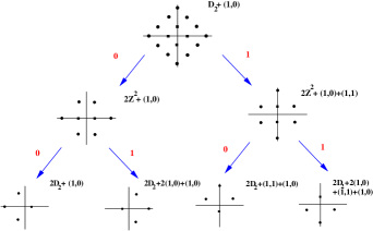
Figure 1: A binary partition of a QAM constellation

2.5 Algebraic properties of binary partitions

The QAM constellations can be represented through a lattice chain $\Lambda|\Lambda_{1}|\Lambda_{2}|\ldots$, where $\Lambda=\mathbb{Z}^{2}$ is the integer lattice. The lattices in the chain are produced with the generator matrix $\mbox{${\bf G}$}^{k}$ where $\mbox{${\bf G}$}=\left[\begin{array}[]{cc}1&1\\ 1&-1\end{array}\right]$. Given this, we can represent the $2^{k}$-QAM constellation as $\Lambda|\Lambda_{k}$, i.e., the coset representatives of $\Lambda$ in $\Lambda_{k}$. The lattice $\Lambda$ can also be written as the set of Gaussian integers $Z[i]=\{a+bi:a,b\in\mathbb{Z}\}$. Similarly we can write the lattice $\Lambda_{k}$ as $\{(a+bi)(1-i)^{k}:a,b\in\mathbb{Z}\}$. This decomposition of the QAM constellation is illustrated in Figure 2. Therefore, using this we can represent any point $s$ in a $2^{L}$-QAM constellation using a $L$-length bit string as

$$s-c(L)\equiv\sum_{l=0}^{L-1}b_{l}(1-i)^{l}\hskip 14.45377pt\mbox{mod }(1-i)^{L},$$ (21)

where we define $f\equiv g\hskip 14.45377pt\mbox{mod }(1-i)^{L}$ if there exist $c,d\in\mathbb{Z}$ such that $f=(c+di)(1-i)^{L}+g$. Also in (21) the constant $c(L)=\frac{1}{2}$ for odd $L$ and $\frac{1}{2}(1+i)$ for even $L$.

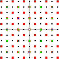
Figure 2: Decomposition for QAM constellations

Binary partitions of PSK constellations are based on a chain of subfields of the cyclotomic field $\mathbb{Q}(\xi_{2^{L}})$ obtained by adjoining $\xi_{2^{L}}=\exp(2\pi i/2^{L})$ to the rational field $\mathbb{Q}$. Analogous to (21), points in the $2^{L}$-PSK constellation can be represented as

$$s=\prod_{l=0}^{L-1}(\xi^{2^{l}})^{b_{l}},$$ (22)

where $\xi=\xi_{2^{L}}=\exp(2\pi i/2^{L})$ and $\xi^{2^{L}}$ is a primitive element for $\mathbb{Q}(\xi_{2^{L-l}})$. Note that $1-\xi$ is prime in $\mathbb{Z}[\xi]$ and the quotient $\mathbb{Z}[\xi]/(1-\xi)$ is the field $\mathbb{Z}_{2}$.

The field $\mathbb{Q}(\xi_{2^{L}})$ is a degree $2^{L-1}$ extension of $\mathbb{Q}$. Every rational number is a quotient $a/b$, where $a,b\in\mathbb{Z}$, and every complex number in $\mathbb{Q}(i)$ is a quotient $a/b$, where $a,b$ are Gaussian integers. In general every complex number in $\mathbb{Q}(\xi_{2^{L}})$ is a quotient $a/b$, where $a,b$ are integer linear combinations of $1,\xi_{2^{L}},\ldots,\xi_{2^{L}}^{2^{L-1}-1}$ and $b\neq 0$. For more details about cyclotomic fields see [20]. Note that $\xi_{2^{L}}^{2^{L-1}}=-1$, so that $\xi_{2^{L}}^{j}=-\xi_{2^{L}}^{2^{L-1}+j}$, for $j=0,1,\ldots,2^{L-1}-1$.

We have a chain of fields

$$\mathbb{Q}=\mathbb{Q}(\xi_{2})\subset\mathbb{Q}(i)=\mathbb{Q}(\xi_{4})\subset\mathbb{Q}(\xi_{8})\ldots\subset\mathbb{Q}(\xi_{2^{L}}).$$

These observations can be used to establish the performance of the multi-level diversity embedded codes [5, 6].

3 Diversity embedded codes for ISI channels

In this section we will first recall the construction of multi-level (non-linear) space-time codes for transmission over flat fading channels that are matched to a binary partition of a QAM or PSK constellation (see [6]). We will give the construction and refer the reader to [6] for proofs of code performance for the flat-fading case. Following this we will use the structure imposed by the ISI on the space time code as in (8) to construct multilevel codes suitable for ISI channels using binary matrices which are constructed in Section 6.

3.1 Multi-Level Constructions for Flat Fading Channels

Given an L-level binary partition of a QAM or PSK signal constellation, a space-time codeword is an array $\mbox{${\bf K}$}=\{\mbox{${\bf K}$}_{1},\mbox{${\bf K}$}_{2},\ldots,\mbox{${\bf K}$}_{L}\}$ determined by a sequence of binary matrices, where matrix, $\mbox{${\bf K}$}_{i}$ specifies the space-time array at level $i$. A multi-level space-time code is defined by the choice of the constituent sets of binary matrices $\mathcal{K}_{1},\mathcal{K}_{2},\ldots,\mathcal{K}_{L}$. These sets of binary matrices provide rank guarantees necessary to achieve the diversity orders required for each message set. For $i=1,\ldots,L$ the binary matrix $\mbox{${\bf K}$}_{i}$ is required to be in the set $\mathcal{K}_{i}$.

Given message sets $\{\mathcal{E}_{i}\}_{i=1}^{L}$, they are mapped to the space-time codeword ${\bf X}$ as shown below.

$$\{\mathcal{E}\}_{i=1}^{L}\stackrel{{\scriptstyle f_{1}}}{{\longrightarrow}}\mbox{${\bf K}$}=\left[\begin{array}[]{ccc}K(1,1)&\ldots&K(1,T)\\ \vdots&\vdots&\vdots\\ K(M_{t},1)&\ldots&K(M_{t},T)\end{array}\right]\stackrel{{\scriptstyle f_{2}}}{{\longrightarrow}}\mbox{${\bf X}$}=\left[\begin{array}[]{ccc}x(1,1)&\ldots&x(1,T)\\ \vdots&\vdots&\vdots\\ x(M_{t},1)&\ldots&x(M_{t},T)\end{array}\right]$$ (29)

where the matrix ${\bf K}$ is specified by $K(m,n)\in\{0,1\}^{\log(|\mathcal{A}|)}$ i.e., binary string and $x(m,n)\in\mathcal{A}$. This construction is illustrated in Figure 3 for a constellation size of $L$ bits.

In summary, given the message set, we first choose the matrices $\mbox{${\bf K}$}_{1},\ldots.\mbox{${\bf K}$}_{L}$. The first mapping $f_{1}$ is obtained by taking matrices and constructing the matrix $\mbox{${\bf K}$}\in{\rm{\bf C}\mkern-9.0mu\rule{0.50003pt}{6.02773pt}\mkern 10.0mu}^{M_{t}\times T}$ each of whose entries is constructed by concatenating the bits from the corresponding entries in the matrices $\mbox{${\bf K}$}_{1},\ldots.\mbox{${\bf K}$}_{L}$ into $L$-length bit-string. This matrix is then mapped to the space-time codeword through a constellation mapper $f_{2}$, for example the set-partition mapping given in Section 2.4. Using this sequence of $L$ matrices, we obtain the space-time codeword as seen in Figure 3.

Figure 3: Schematic representation of the multi-level code construction.

For flat fading channels the sets $\mathcal{K}_{l},l=1,\ldots,L$ are binary $M_{t}\times T$ matrices such that for any distinct pair of matrices $\mbox{${\bf A}$},\mbox{${\bf B}$}\in\mathcal{K}$ the rank of $\mbox{${\bf A}$}-\mbox{${\bf B}$}$ is at least $M_{t}-d$. The size of $\mathcal{K}$ is at most $2^{(d+1)T}$ since the first $d+1$ rows of ${\bf A}$ and ${\bf B}$ must be distinct, and there is a classical example [8] that achieves the bound (this construction was also given in [14, 15]).

With the rate achieved on the $l^{th}$ layer defined as $R_{l}=\frac{1}{T}\log|\mathcal{K}_{l}|$ it can be shown [6] that this construction for QAM constellations achieves the rate-diversity tuple $(R_{1},M_{r}d_{1}(\nu+1),\ldots,$ $R_{L},M_{r}d_{L}(\nu+1))$, with the overall equivalent single layer code achieving rate-diversity point, $(\sum_{l}R_{l},M_{r}d_{L}(\nu+1))$. Optimal decoding employs a maximum-likelihood decoder which jointly decodes the message sets. This is the decoder for which the performance is summarized in Theorem 4.

Theorem 4

[6] Let $\mathcal{C}$ be a multi-level space-time code for a QAM or $M$-PSK constellation of size $2^{L}$ with $M_{t}$ transmit antennas that is determined by constituent sets of binary matrices $\mathcal{K}_{l},l=1,\ldots,L$ with binary rank guarantees $d_{1}\geq d_{2}\ldots\geq d_{L}$. For joint maximum-likelihood decoding, the input bits that select the codeword from the $i$th matrix $\mathcal{K}_{i}$ are guaranteed diversity $d_{i}M_{r}$ in the complex domain when transmitted over a flat fading channel.

3.2 Multi-Level Construction for ISI Channels

In this section we use the idea of multi-level diversity embedded codes for flat fading channels as in Section 3.1 and the structure imposed by the ISI on the space time code as in (8) to motivate construction and analysis of a class of binary matrices as follows.

We apply the idea suggested by the constructions of multi-level codes for flat-fading channels to the fading ISI case. We do this by applying a zero padding as seen in (11) along with mappings of binary matrices to the transmit signal alphabet. That is, we use the mapping given in (29) for a block size of $T$ with the constraint that the last $\nu$ entries of the mapping lead to given alphabets (taken to be zero without loss of generality). This is combined with binary sets $\mathcal{K}_{\nu,d}$, which we specify in definition 5. This means that over a time period $T$, we transmit a sequence ${\bf x}[0],{\bf x}[1],\ldots,{\bf x}[T-\nu-1]$ which are mapped from the inputs bits using a structure given in (29). Therefore, given that we transmit the sequence shown in (31),

$$\mathbf{X}^{(1)} =\left[\begin{array}[]{ccccccc}{\bf x}[0]&{\bf x}[1]&\ldots&{\bf x}[T-\nu-1]&0&\ldots&0\end{array}\right],$$ (31)

we need a mapping from a binary matrix as in (29). For a constellation of size $2^{L}$, we do this by taking message sets $\{\mathcal{E}_{i}\}_{i=1}^{L}$ and mapping them to a codeword with the structure given in (31) as follows,

$$\{\mathcal{E}_{i}\}_{i=1}^{L}\stackrel{{\scriptstyle f_{1}}}{{\longrightarrow}}\mbox{${\bf K}$}^{(1)}=\left[\begin{array}[]{ccc}K(1,1)&\ldots&K(1,T)\\ \vdots&\vdots&\vdots\\ K(M_{t},1)&\ldots&K(M_{t},T)\end{array}\right]\stackrel{{\scriptstyle f_{2}}}{{\longrightarrow}}\mbox{${\bf X}$}^{(1)}=\left[\begin{array}[]{ccccccc}{\bf x}[0]&{\bf x}[1]&\ldots&{\bf x}[T-\nu-1]&0&\ldots&0\end{array}\right]$$ (36)

where the $(m,n)^{th}$ entry of $\mbox{${\bf K}$}^{(1)}$ is given by $K(m,n)\in\{0,1\}^{\log(|\mathcal{A}|)}$ i.e., binary string. Since the mapping $f_{2}$ is just the set-partitioning mapping specified in Section 2.4, we need the last $\nu$ columns of $\mbox{${\bf K}$}^{(1)}$ to be given constants for all choices of the message sets $\{\mathcal{E}_{i}\}_{i=1}^{L}$. That is, we need the following structure for the matrix $\mbox{${\bf K}$}^{(1)}$,

$$\mathbf{K}^{(1)} =\left[\begin{array}[]{ccccccc}{\bf k}[0]&{\bf k}[1]&\ldots&{\bf k}[T-\nu-1]&\mathbf{0}&\ldots&\mathbf{0}\end{array}\right],$$ (38)

where, as before, $\{{\bf k}[i]\}$ are columns of binary strings of length $L$, and with no loss of generality, we have specified the last $\nu$ columns of $\mbox{${\bf K}$}^{(1)}$ to be the zero strings.

Given that we have an ISI channel, the transmitted codeword with the structure given in (31) gives an equivalent codeword matrix with a Toeplitz structure, as specified in (8). This Toeplitz structure is equivalent to mapping a Toeplitz matrix ${\bf K}$ of binary strings with the structure

$${\bf K} =\left[\begin{array}[]{ccccccc}{\bf k}[0]&{\bf k}[1]&\ldots&{\bf k}[T-\nu-1]&\mathbf{0}&\ldots&\mathbf{0}\\ \mathbf{0}&{\bf k}[0]&{\bf k}[1]&\ldots&{\bf k}[T-\nu-1]&\mathbf{0}&\mathbf{0}\\ \ldots&&\vdots&\ddots&.&.&\vdots\\ \mathbf{0}&\ldots&\mathbf{0}&{\bf k}[\mathbf{0}]&{\bf k}[1]&\ldots&{\bf k}[T-\nu-1]\end{array}\right],$$ (43)

to ${\bf X}$ using the constellation mapping $f_{2}$. Therefore, as in the flat fading case, given the message set, we first choose the binary matrices $\mbox{${\bf K}$}_{1}^{(1)},\ldots.\mbox{${\bf K}$}_{L}^{(1)}$, each of which have the structure specified below in (45). These put together give us the matrix of binary strings $\mbox{${\bf K}$}^{(1)}$. This in turn, due to the ISI channel, is relates to ${\bf K}$, the Toeplitz matrix of binary strings, given above in (43). Therefore, the choice of matrices $\mbox{${\bf K}$}_{1}^{(1)},\ldots.\mbox{${\bf K}$}_{L}^{(1)}$, for the ISI case, naturally is equivalent to a choice of Toeplitz binary matrices, $\mbox{${\bf K}$}_{1},\ldots.\mbox{${\bf K}$}_{L}$, as specified in (50) below.

Therefore, for the multi-level coding structure we have used, analogous to the flat fading case studied in [6], we need to study the rank properties of sets of binary Toeplitz matrices as specified below. Consider the matrix $\mathbf{B}\in\mathbb{F}_{2}^{M_{t}\times T}$, with the following structure,

$$\mathbf{B} =\left[\begin{array}[]{ccccccc}{\bf c}[0]&{\bf c}[1]&\ldots&{\bf c}[T-\nu-1]&\mathbf{0}&\ldots&\mathbf{0}\end{array}\right],$$ (45)

where $\mathbf{c}[n]\in\mathbb{F}_{2}^{M_{t}\times 1},\,\,n=0,\ldots,T-\nu-1$. We define a mapping $\Theta:\mathbb{F}_{2}^{M_{t}\times T}\rightarrow\mathbb{F}_{2}^{(\nu+1)M_{t}\times T}$ by,

$$\Theta\left(\mathbf{B}\right) =\left[\begin{array}[]{ccccccc}{\bf c}[0]&{\bf c}[1]&\ldots&{\bf c}[T-\nu-1]&\mathbf{0}&\ldots&\mathbf{0}\\ \mathbf{0}&{\bf c}[0]&{\bf c}[1]&\ldots&{\bf c}[T-\nu-1]&\mathbf{0}&\mathbf{0}\\ \ldots&&\vdots&\ddots&.&.&\vdots\\ \mathbf{0}&\ldots&\mathbf{0}&{\bf c}[\mathbf{0}]&{\bf c}[1]&\ldots&{\bf c}[T-\nu-1]\end{array}\right]$$ (50)

Definition 5

Define $\mathcal{K}_{\nu,d}\subset\{\mathbf{B}:\mathbf{B}\in\mathbb{F}_{2}^{M_{t}\times T}\}$ to be the set of binary matrices of the form given in (45) if for some fixed $T_{thr}$ they satisfy the following properties for $T\geq T_{thr}$.

• For any distinct pair of matrices $\mbox{${\bf A}$},\mbox{${\bf B}$}\in\mathcal{K}_{\nu,d}$ the rank of $\left[\Theta(\mbox{${\bf A}$})-\Theta(\mbox{${\bf B}$})\right]$ is at least $d(\nu+1)$.

• $|\mathcal{K}_{\nu,d}|\geq 2^{T(M_{t}-d+1)-\nu M_{t}}$.

Note that in Section 3.1 the first step in code construction was constructing the sets $\mathcal{K}_{l},l=1,\ldots,L$ from which the matrices $\mbox{${\bf K}$}_{1},\ldots.\mbox{${\bf K}$}_{L}$ were chosen. In the case of flat fading channels there are constructions by [8] but these do not satisfy the rank guarantee properties in Definition 5. We will postpone the construction of such sets of binary matrices $\{\mathcal{K}_{\nu,d}\}$ to Section 6, where we show that we can set $T_{thr}=R\nu+(M_{t}-1)(\nu+1)(2^{R}-1)$. More formally, in Section 6, we show that,

Lemma 6

For block size $T\geq T_{thr}=R\nu+(M_{t}-1)(\nu+1)(2^{R}-1)$, there exist sets of binary matrices $\mathcal{K}_{\nu,d}$ which satisfy the requirements of Definition 5.

Adapted easily from [6] we can state the formal construction guarantee for the diversity embedded code for transmission over the ISI channel as follows.

Theorem 7

Let $\mathcal{C}$ be a multi-level space-time code for a QAM or PSK constellation of size $2^{L}$ with $M_{t}$ transmit antennas that is determined by constituent sets of binary matrices $\mathcal{K}_{l}=\mathcal{K}_{\nu,d_{l}},l=1,\ldots,L$, such that $d_{1}\geq d_{2}\ldots\geq d_{L}$. For joint maximum-likelihood decoding, the input bits that select the codeword from the $l$th set $\mathcal{K}_{l}$ are guaranteed diversity $d_{l}(\nu+1)M_{r}$ in the complex domain when transmitted over an ISI channel with $\nu+1$ taps.

The proof of the Theorem 7 follows from the same techniques as in [6] by mapping binary matrices with desired rank guarantees to rank guarantees in complex domain. In particular, given sets of (Toeplitz) binary matrices $\mathcal{K}_{l}=\mathcal{K}_{\nu,d_{l}},l=1,\ldots,L$, which have rank guarantees of $\{d_{l}\}$, given the set-partitioning mapping $f_{2}$, we can lift the binary rank properties to the complex domain. Therefore, the main challenge, addressed in this paper, is the construction of such sets of binary matrices with rank guarantees.

Therefore the codewords from $l$th layer achieve a rate $R_{l}=\frac{1}{T}\log|\mathcal{K}_{\nu,d_{l}}|$ and diversity order $d_{l}(\nu+1)M_{r}$. From Definition 5 it follows that the size of $\mathcal{K}_{\nu,d_{l}}$ can be made at least as large as $2^{T\left(M_{t}-d_{l}+1\right)-\nu M_{t}}$. Similar to [6] this construction for QAM constellations achieves the rate-diversity tuple $(R_{1},M_{r}d_{1}(\nu+1),\ldots,R_{L},M_{r}d_{L}(\nu+1))$, with the overall equivalent single layer code achieving rate-diversity point, $(\sum_{l}R_{l},M_{r}d_{L}(\nu+1))$.

In particular, we can construct a space-time code by choosing identical diversity requirements for all the layers, i.e., $d_{1}=d_{2}=\ldots=d_{L}$. From this we conclude that the rate diversity tradeoff for the ISI channel can be characterized as follows:

Theorem 8

(Rate Diversity Tradeoff for ISI Channels) Consider transmission over a $\nu$ tap ISI channel with $M_{t}$ transmit antennas from a QAM or PSK signal constellation $\mathcal{A}$ with $|\mathcal{A}|=2^{L}$ and communication over a time period $T$ such that $T\geq T_{thr}$. For diversity order $d_{isi}=d(\nu+1)M_{r}$, the rate diversity tradeoff is given by,

$$(M_{t}-d+1)-\frac{\nu}{T}M_{t} \leq R^{eff}\leq\left(M_{t}-d+1\right).$$

The lower bound follows directly from Theorem 7 and the upper bound follows from lemma 3. Note that the bounds in the above theorem are tight as $T\rightarrow\infty$.

4 Diversity Embedded Trellis Codes

The construction of diversity embedded trellis codes for ISI channels is quite similar to the construction of block codes. Again the idea is to construct binary convolutional codes with the following properties.

Definition 9

Define $\mathcal{P}_{\nu,d}\subset\{\mathbf{B}:\mathbf{B}\in\mathbb{F}_{2}^{M_{t}\times T}\}$ to be the set of binary matrices of the form given in (45) if for some fixed $T_{thr}$ they satisfy the following properties for $T\geq T_{thr}$

• For any distinct pair of matrices $\mbox{${\bf A}$},\mbox{${\bf B}$}\in\mathcal{P}_{\nu,d}$ the rank of $\Gamma(\mbox{${\bf A}$})-\Gamma(\mbox{${\bf B}$})$ is at least $d(\nu+1)$.

• $\log|\mathcal{P}_{\nu,d}|\geq R(T-\nu-(\nu+1)(M_{t}-1)(2^{R}-1)(2^{R-1}))$, where $R=M_{t}-d+1$.

Using these sets of matrices obtained by appropriately choosing the underlying convolutional codes the diversity embedding properties are ensured.

We will postpone the construction of such sets of binary matrices to Section 4.1 where using Lemma 6 along with particular choices of convolutional codes we show the following result.

Lemma 10

For block size $T\geq T_{thr}=(2^{R}-1)\nu+(2^{R}-1)(\nu+1)\left((M_{t}-2)(2^{R}-1)+R\right)$, where $R=M_{t}-d+1$, there exist sets of binary matrices $\mathcal{P}_{\nu,d}$ which satisfy the requirements of Definition 9.

As in the case of block codes in Section 3, given a $L$-level binary partition of a QAM or PSK signal constellation, a diversity embedded convolutional space-time codeword is defined by an array $\mbox{${\bf P}$}=\{\mbox{${\bf P}$}^{(1)},\mbox{${\bf P}$}^{(2)},\ldots,\mbox{${\bf P}$}^{(L)}\}$ determined by a sequence of binary matrices, where matrix, $\mbox{${\bf P}$}^{(i)}$ specifies the space-time array at level $i$. Adapted easily from [6] we can state the formal construction guarantee for the diversity embedded trellis code for ISI channels as follows.

Theorem 11

Let $\mathcal{C}$ be a multi-level space-time code for a QAM or PSK constellation of size $2^{L}$ with $M_{t}$ transmit antennas that is determined by constituent sets of binary matrices $\mathcal{P}_{l}=\mathcal{P}_{\nu,d_{l}},l=1,\ldots,L$, such that $d_{1}\geq d_{2}\ldots\geq d_{L}$. For joint maximum-likelihood decoding, the input bits that select the codeword from the $l$th set $\mathcal{P}_{l}$ are guaranteed diversity $d_{l}(\nu+1)M_{r}$ in the complex domain.

The proof of the Theorem 11 follows from the same techniques as in [6] by mapping binary matrices with desired rank guarantees to rank guarantees in complex domain. As in the proof of Theorem 7, the main difficulty is in constructing these sets of binary matrices with thee given rank guarantees, using convolutional codes. We give such a construction in Section 4.1. Therefore the codewords from $l$th layer achieve a rate $R_{l}=\frac{1}{T}\log|\mathcal{P}_{\nu,d_{l}}|$ and diversity order $d_{l}(\nu+1)M_{r}$. From Definition 9 it follows that the size of $\mathcal{P}_{\nu,d_{l}}$ can be made at least as large as $2^{R(T-\nu-(\nu+1)(M_{t}-1)(2^{R}-1)(2^{R-1}))}$, which in the limit as $T\rightarrow\infty$ tends to $2^{R}$. Similar to [6] this construction for QAM constellations achieves the rate-diversity tuple $(R_{1},M_{r}d_{1}(\nu+1),\ldots,R_{L},M_{r}d_{L}(\nu+1))$, with the overall equivalent single layer code achieving rate-diversity point, $(\sum_{l}R_{l},M_{r}d_{L}(\nu+1))$.

We illustrate the idea by examining the construction for each of the layers. The construction is shown in Figure 4. Given the input stream for each layer $i$, the first block in the figure maps these inputs to the coefficients of $R_{i}$ polynomials $u_{i,j}(D),j=1,\ldots,R_{i}$ in $\mathbb{F}_{2}[D]$. The second block multiplies the input vector $\{u_{i,j}(D)\}_{j=1}^{R_{i}}$ by the generator matrix ${\bf G}_{i}(D)$, with special structure which we define in the following subsection, and generates a vector ${\bf u}_{i}(D)$ of polynomials. The final block $\Omega$ then maps this vector ${\bf p}_{i}(D)$ to a binary matrix ${\bf P}_{i}\in\mathbb{F}_{2}^{M_{t}\times T}$.

We define the set $\mathcal{P}_{i}=\mathcal{P}_{\nu,i}$ to be the set of all output matrices ${\bf P}_{i}$ for all possible inputs on the stream $i$. Note that these sets satisfy the properties in Definition 9.

Figure 4: Binary matrices for each layer

4.1 Binary Convolutional Codes

Explicit construction of full diversity maximum rate binary convolutional codes was first shown in [11]. This was extended for general points on the rate diversity tradeoff for flat fading channels in [15]. We will give constructions for such sets of binary matrices for ISI channels in this section.

Consider the construction for a particular layer above. We will see the construction of rate $R$ symbols per transmission, and rank distance of $(\nu+1)(M_{t}-R+1)$ binary codes for transmission over the ISI channel. Represent the generator matrix or transfer function matrix ${\bf G}$ for this code by an $R\times M_{t}$ generator matrix given by,

$${\bf G} =\left[\begin{array}[]{cccc}g_{1}^{(1)}(D)&g_{1}^{(2)}(D)&\cdots&g_{1}^{(M_{t})}(D)\\ g_{2}^{(1)}(D)&g_{2}^{(2)}(D)&\cdots&g_{2}^{(M_{t})}(D)\\ \vdots&\ddots&\ddots&\vdots\\ g_{R}^{(1)}(D)&g_{R}^{(2)}(D)&\cdots&g_{R}^{(M_{t})}(D)\end{array}\right]$$ (55)

Denoting $\xi=D^{(\nu+1)(2^{R}-1)}$ we choose

$$g_{l}^{(q)}(D)=\xi^{(q-1)2^{(l-1)}}.$$ (56)

The input message polynomial is represented by the vector of message polynomial

$${\bf u}(D) =\left[\begin{array}[]{cccc}u_{1}(D)&u_{2}(D)&\cdots&u_{R}(D)\end{array}\right]^{t}$$ (58)

where $u_{i}(D)\in\mathbb{F}_{2}[D]$. The code polynomial vector is given by

$${\bf p}(D) ={\bf G}^{t}(D){\bf u}(D)$$

$$=\left[\begin{array}[]{cccc}p_{1}(D)&p_{2}(D)&\cdots&p_{M_{t}}(D)\end{array}\right]^{t}.$$ (60)

The $M_{t}\times T$ code matrix which is actually transmitted on the antenna is given by

$${\bf P} =\left[\begin{array}[]{ccc}p_{1}^{0}&\cdots&p_{1}^{T-1}\\ \vdots&\ddots&\vdots\\ p_{M_{t}}^{0}&\cdots&p_{M_{t}}^{T-1}\end{array}\right]$$ (64)

where $p_{i}^{j}$ is the $j^{th}$ coefficient of the polynomial $p_{i}$ in (4.1). We make a distinction between ${\bf p}(D)$ which is a vector of polynomials in $D$ and ${\bf P}$ which is a binary matrix. This mapping is denoted by $\Omega$ i.e. $\Omega({\bf p}(D))={\bf P}$

Note that in order that the matrix ${\bf P}$ satisfies the structure in (45) we require the $\nu$ largest coefficients of each $p_{i}(D)$ in (4.1) to be zero, i.e.,

$$p_{i}^{j} =0\qquad\forall\,i\in\{1,\ldots,M_{t}\}\ {\rm and}\ \forall\,j\in\{T-\nu-1,\ldots,T-1\}.$$ (65)

With this constraint we get that,

$$deg(u_{i}(D)) \leq T-1-\nu-\max_{u,v}deg(g_{u}^{(v)})$$

$$=T-1-\nu-(\nu+1)(M_{t}-1)(2^{R}-1)(2^{R-1})$$

where the last equality follows from our particular choice of $g_{u}^{(v)}$ given in (56). Note that this convolutional code corresponds to a effective rate of

$$R^{eff} =\frac{\log\left(2^{T-1-\nu-(\nu+1)(M_{t}-1)(2^{R}-1)(2^{R-1})+1}\cdot 2^{R}\right)}{T}$$

$$=\frac{R\left(T-\nu-(\nu+1)(M_{t}-1)(2^{R}-1)(2^{R-1})\right)}{T}\quad bits/Tx$$ (66)

which asymptotically tends to $R$ as $T\rightarrow\infty$.

Also, observe that,

$$\Theta({\bf P}) =\left[\begin{array}[]{c}\Omega({\bf p}(D))\\ \Omega(D{\bf p}(D))\\ \vdots\\ \Omega(D^{\nu}{\bf p}(D))\end{array}\right].$$ (71)

From this we can conclude that,

$$\Theta({\bf P})) =\Omega\left(\tilde{{\bf G}}^{t}(D){\bf u}(D)\right)$$

where $\tilde{{\bf G}}\in\mathbb{F}_{2}^{R\times(\nu+1)M_{t}}$ is given by,

$$\tilde{{\bf G}} =\left[\begin{array}[]{ccccccccccc}g_{1}^{(1)}(D)&g_{1}^{(2)}(D)&\cdots&g_{1}^{(M_{t})}(D)&Dg_{1}^{(1)}(D)&\cdots&Dg_{1}^{(M_{t})}(D)&\cdots&D^{\nu}g_{1}^{(1)}(D)&\cdots&D^{\nu}g_{1}^{(M_{t})}(D)\\ g_{2}^{(1)}(D)&g_{2}^{(2)}(D)&\cdots&g_{2}^{(M_{t})}(D)&Dg_{2}^{(1)}(D)&\cdots&Dg_{2}^{(M_{t})}(D)&\cdots&D^{\nu}g_{2}^{(1)}(D)&\cdots&D^{\nu}g_{2}^{(M_{t})}(D)\\ \vdots&\ddots&\ddots&\vdots&&&&&&&\\ g_{R}^{(1)}(D)&g_{R}^{(2)}(D)&\cdots&g_{R}^{(M_{t})}(D)&Dg_{R}^{(1)}(D)&\cdots&Dg_{R}^{(M_{t})}(D)&\cdots&D^{\nu}g_{R}^{(1)}(D)&\cdots&D^{\nu}g_{R}^{(M_{t})}(D)\end{array}\right]$$ (76)

With our particular choice of $g_{l}^{(q)}(D)$, given in (56), we can write this as,

$$\tilde{{\bf G}}^{t} =\left[\begin{array}[]{cccc}1&\ldots&1&1\\ \xi&\xi^{2}&\ldots&\xi^{2^{R-1}}\\ \xi^{2}&(\xi^{2})^{2}&\ldots&(\xi^{2})^{2^{R-1}}\\ \vdots&&\vdots&\\ \xi^{(M_{t}-1)}&(\xi^{(M_{t}-1)})^{2}&\ldots&(\xi^{(M_{t}-1)})^{2^{R-1}}\\ D&\ldots&D&D\\ &\vdots&&\vdots\\ D\xi^{(M_{t}-1)}&D(\xi^{(M_{t}-1)})^{2}&\ldots&D(\xi^{(M_{t}-1)})^{2^{R-1}}\\ &\vdots&&\vdots\\ &\vdots&&\vdots\\ D^{\nu}\xi^{(M_{t}-1)}&D^{\nu}(\xi^{(M_{t}-1)})^{2}&\ldots&D^{\nu}(\xi^{(M_{t}-1)})^{2^{R-1}}\\ \end{array}\right]$$ (88)

Define the polynomial

$$f(x)=\sum_{l=0}^{R-1}u_{l}(D)x^{2^{l}},$$ (89)

where $\{u_{l}(D)\}_{l=0}^{R-1}\in\mathbb{F}_{2}[D]$. Then from (88) with $\xi=D^{(\nu+1)(2^{R}-1)}$ we have,

$$\tilde{{\bf G}}^{t}(D){\bf u}(D) =\left[\begin{array}[]{c}f(1)\\ f(\xi)\\ \vdots\\ f(\xi^{(M_{t}-1)})\\ Df(1)\\ \vdots\\ D^{\nu}f(\xi^{(M_{t}-1)})\end{array}\right]$$

The proof now that the left null space of $\Omega\left(\tilde{{\bf G}}^{t}(D){\bf u}(D)\right)$ over $\mathbb{F}_{2}$ is of dimension at most $d(\nu+1)$ is the same as the proof of Theorem 21 by choosing $T$ such that,

$$T \geq(2^{R}-1)\nu+(2^{R}-1)(\nu+1)\left((M_{t}-2)(2^{R}-1)+R\right).$$

Therefore, given the result of Theorem 21, which is proved in Section 6.3, we can prove the rank guarantees of the convolutional codes.

5 Rate Guarantees

In this section we will give background needed for construction of binary codes $\mathcal{K}_{\nu,d}$ with properties given in Definition 5. We start in Section 5.1 with a representation of $\mathcal{K}_{\nu,d}$ in terms of polynomials over $\mathbb{F}_{2^{T}}$ which will be useful in proving the construction of binary codes $\mathcal{K}_{\nu,d}$. In Section 5.2 we will list some definitions which we will use in proving rank guarantees in Section 6. Note that these definitions are not required for constructing $\mathcal{K}_{\nu,M_{t}}$, i.e., maximal rank sets, for which the proof is much simpler as seen in Section 6.1. Finally in Section 5.3 we will show that $|\mathcal{K}_{\nu,d}|\geq 2^{RT-\nu M_{t}}$, where $R=M_{t}-d+1$. The rank properties of $\mathcal{K}_{\nu,d}$ are given in Section 6.

5.1 Polynomial representation

Given a rate $R$, we define the linearized polynomial

$$f(x)=\sum_{l=0}^{R-1}f_{l}x^{2^{l}},$$ (90)

where $\{f_{l}\}_{l=0}^{R-1}\in\mathbb{F}_{2^{T}}$. To develop the binary matrices with structure given in (45), we define $\mbox{${\bf c}$}_{f}\in\mathbb{F}_{2^{T}}^{M_{t}}$

$$\mathbf{c}_{f} =\left[\begin{array}[]{cccc}f(1)&f(\xi)&\ldots&f(\xi^{(M_{t}-1)})\end{array}\right]^{t}.$$ (92)

where $\xi=\alpha^{(2^{R}-1)(\nu+1)}$, and $\alpha$ is a primitive element of $\mathbb{F}_{2^{T}}$. Let $\mathbf{f}^{(0)}(\xi^{i})$ and $\mathbf{f}^{(k)}(\xi^{i})$ be the representations of $f(\xi^{i})$ and $\alpha^{k}f(\xi^{i})$ in the basis $\{\alpha^{0},\alpha^{1},\ldots,\alpha^{T-1}\}$ respectively i.e., $\mathbf{f}^{(0)}(\xi^{i}),\mathbf{f}^{(k)}(\xi^{i})\in\mathbb{F}_{2}^{1\times T}$ . We obtain a matrix representation $\mbox{${\bf C}$}_{f}\in\mathbb{F}_{2}^{M_{t}\times T}$ of $\mathbf{c}_{f}$ as,

$$\mathbf{C}_{f} =\left[\begin{array}[]{cccc}\mathbf{f}^{(0)t}(1)&\mathbf{f}^{(0)t}(\xi)&\ldots&\mathbf{f}^{(0)t}(\xi^{(M_{t}-1)})\end{array}\right]^{t}.$$ (94)

Now, in order to get the structure required in (45), we need to study the requirements of $f$ so that the last $\nu$ elements in $\mathbf{C}_{f}$ are $0$ for all the $M_{t}$ rows. Note that the $j^{th}$ row of $\mathbf{C}_{f}$ is given by the binary expansion of $f(\xi^{j-1})\in\mathbb{F}_{2^{T}}$ in terms of the basis $\{\alpha^{0},\alpha,\ldots,\alpha^{T-1}\}$, where $\alpha$ is a primitive element of $\mathbb{F}_{2^{T}}$. The coefficients in this basis expansion can be obtained using the trace operator described below for completeness.

Consider an extension field $\mathbb{F}_{2^{T}}$ of the base field $\mathbb{F}_{2}$. If $\alpha\in\mathbb{F}_{2^{T}}$ is a primitive element of $\mathbb{F}_{2^{T}}$ then $(\alpha^{0},\alpha^{1},\ldots,\alpha^{T-1})$ form a basis of $\mathbb{F}_{2^{T}}$ over $\mathbb{F}_{2}$ and any element $\beta\in\mathbb{F}_{2^{T}}$ can be uniquely represented in the form,

$$\beta=\beta_{0}\alpha^{0}+\beta_{1}\alpha^{1}+\ldots\beta_{T-1}\alpha^{T-1}\quad{\rm with}\ \beta_{i}\in\mathbb{F}_{2},\ {\rm for}\ 0\leq i\leq(T-1).$$

To solve for the coefficients $\beta_{i}$ we will use the trace function and trace dual bases. Note that for any element $\beta\in\mathbb{F}_{2^{T}}$ the trace of the element $\beta$ relative to the base field $\mathbb{F}_{2}$ is defined as,

$${\rm Tr}_{2^{T}/2}\left(\beta\right) =\beta+\beta^{2}+\beta^{2^{2}}+\ldots+\beta^{2^{T-1}}.$$

Given that $\beta,\tilde{\beta}\in\mathbb{F}_{2^{T}}$ the trace function satisfies the following properties,

• ${\rm Tr}_{2^{T}/2}(\beta)\in\mathbb{F}_{2}$.

• ${\rm Tr}_{2^{T}/2}(\beta+\tilde{\beta})={\rm Tr}_{2^{T}/2}(\beta)+{\rm Tr}_{2^{T}/2}(\tilde{\beta})$.

• ${\rm Tr}_{2^{T}/2}(\lambda\beta)=\lambda{\rm Tr}_{2^{T}/2}(\beta)$, if $\lambda\in\mathbb{F}_{2}$.

Also given the basis $(\alpha^{0},\alpha^{1},\ldots,\alpha^{T-1})$ the corresponding trace dual basis $(\theta_{0},\theta_{1},\ldots,\theta_{T-1})$ is defined to be the unique set of elements which satisfy the following relation for $0\leq i,j\leq(T-1)$,

$${\rm Tr}_{2^{T}/2}\left(\theta_{i}\alpha^{j}\right) =\begin{cases}0&{\rm for}\ i\neq j\\ 1&{\rm for}\ i=j\end{cases}$$

The fact that the trace dual basis exists and is unique can be found in standard references such as [13, 16]. Therefore given $\beta\in\mathbb{F}_{2^{T}}$, we can find $\beta_{i}$ by using the properties of the trace function and noting that,

$${\rm Tr}_{2^{T}/2}\left(\theta_{i}\beta\right) ={\rm Tr}_{2^{T}/2}\left(\theta_{i}\sum_{j=0}^{T-1}\beta_{j}\alpha^{j}\right)=\sum_{j=0}^{T-1}{\rm Tr}_{2^{T}/2}\left(\theta_{i}\beta_{j}\alpha^{j}\right)=\sum_{j=0}^{T-1}\beta_{j}{\rm Tr}_{2^{T}/2}\left(\theta_{i}\alpha^{j}\right)=\beta_{i}$$

where the last equality follows from the definition of the trace dual basis. Therefore binary matrix $\mathbf{B}$ given in (45) can be represented in terms of the set $\mathcal{S}$ defined as

$$\mathcal{S} =\left\{f:f\in\mathbb{F}_{2^{T}}^{R},{\rm Tr}_{2^{T}/2}\left(\theta_{i}f(\xi^{j})\right)=0\,\,\forall i\in\{T-\nu,\ldots,T-1\}\,\,{\rm and}\,\,\forall j\in\{1,\ldots,M_{t}\}\right\}$$ (95)

Associate to $f\in\mathcal{S}$ the codeword vector $\mathbf{u}_{f}\in\mathbb{F}_{2^{T}}^{(\nu+1)M_{t}\times 1}$ given by,

$$\mathbf{u}_{f} =\left[\begin{array}[]{cccc}\mathbf{c}^{t}_{f}&\alpha\mathbf{c}^{t}_{f}&\ldots&\alpha^{\nu}\mathbf{c}^{t}_{f}\end{array}\right]^{t}$$ (97)

Associate with every such codeword $\mathbf{u}_{f}$ the codeword matrix $\mathbf{U}_{f}\in\mathbb{F}_{2}^{(\nu+1)M_{t}\times T}$ given by the representation of each element of $\mathbf{u}_{f}$ in the basis $\{\alpha^{0},\alpha^{1},\ldots,\alpha^{T-1}\}$.

Since $f\in\mathcal{S}$ we know that the last $\nu$ elements in $\mathbf{C}_{f}$ are $0$ for all the $M_{t}$ rows. Therefore we can see that $\mathbf{f}^{(k)}(\xi^{i})$ is a cyclic shift by $k$ positions of $\mathbf{f}(\xi^{i})$. Hence, for $i\in\{0,1,\ldots,\nu\}$ we can write,

$$\mathbf{C}_{f}^{(i)} =\left[\begin{array}[]{cccc}\mathbf{f}^{(i)t}(1)&\mathbf{f}^{(i)t}(\xi)&\ldots&\mathbf{f}^{(i)t}(\xi^{(M_{t}-1)})\end{array}\right]^{t},$$ (99)

where $\mathbf{C}_{f}^{(i)}$ represents the matrix obtained by a cyclic shift of all the rows of the matrix $\mathbf{C}_{f}$ by $i$ positions.

For transmission over an ISI channel, as seen in Section 3.2, it can be shown from equation (8) that the effective binary transmitted codeword matrix for a particular $f$ is of the form

$$\mathbf{U}_{f} =\left[\begin{array}[]{cccc}\mathbf{C}_{f}^{t}&\mathbf{C}_{f}^{(1)t}&\ldots&\mathbf{C}_{f}^{(\nu)t}\end{array}\right]^{t}$$ (101)

Clearly we see that $\mathcal{K}_{\nu,d}=\left\{\mathbf{C}_{f}:f\in\mathcal{S},\mbox{rank}(\mbox{${\bf U}$}_{f})\geq d(\nu+1)\right\}$. We will show in 6.3 that indeed for $R=M_{t}-d+1$ that $\mathcal{K}_{\nu,d}=\left\{\mathbf{C}_{f}:f\in\mathcal{S}\right\}$, i.e., $\mbox{rank}(\mbox{${\bf U}$}_{f})\geq d(\nu+1),\forall f\in\mathcal{S}$.

5.2 Notation and Definitions

We will need the following definitions in the construction of the basis vectors of the null space of $\mbox{${\bf U}$}_{f}$.

1. We define a set $\Gamma\subseteq\mathbb{F}_{2^{T}}$ which will be used extensively in the proof in Section 6 as,

   $$\Gamma=\{\gamma\in\mathbb{F}_{2^{T}}:\gamma=\sum_{t=0}^{\nu}\delta_{t}\alpha^{t},\delta_{t}\in\mathbb{F}_{2}\}.$$ (102)

2. Given a binary vector $\mathbf{b}\in\mathbb{F}_{2}^{(\nu+1)M_{t}\times 1}$ define $\Psi:\mathbb{F}_{2}^{(\nu+1)M_{t}\times 1}\rightarrow\Gamma^{1\times M_{t}}$ as,

   $$\Psi(\mathbf{b}) =\underbrace{\left[\begin{array}[]{ccc}\sum_{i=0}^{\nu}b_{iM_{t}+1}\alpha^{i}&\ldots&\sum_{i=0}^{\nu}b_{iM_{t}+M_{t}}\alpha^{i}\end{array}\right]}_{\mathbf{g}}$$ (104)

   Note that the mapping $\Psi$ is a one-to-one mapping between $\mathbf{b}$ and $\mathbf{g}$, due to the linear independence of $\{\alpha^{0},\alpha,\ldots,\alpha^{\nu}\}$.

3. For a given fixed $\mathbf{c}_{f}\in\mathbb{F}_{2^{T}}^{M_{t}\times 1}$ define $\mathcal{G}_{f}\subseteq\Gamma^{1\times M_{t}}$ such that,

   $$\mathcal{G}_{f}=\{\mathbf{g}\in\Gamma^{1\times M_{t}}:\mathbf{g}\mathbf{c}_{f} =0\}$$ (105)

4. Motivated by the mapping in (104), for each $\mathbf{g}^{(i)}\in\mathcal{G}_{f}$ we will use the following representation:

   $$\mathbf{g}^{(i)} = \left[\begin{array}[]{ccc}g_{0}^{(i)}&\ldots&g_{M_{t}-1}^{(i)}\end{array}\right]$$ (107)

   $$g_{k}^{(i)} = \sum_{j=0}^{\nu}\delta_{k,j}^{(i)}\alpha^{j}\quad{\rm where}\,\,\delta_{k,j}^{(i)}\in\mathbb{F}_{2}$$

5. For an element $\gamma\in\Gamma$ given by $\gamma=\sum_{j=0}^{\nu}\delta_{j}\alpha^{j}$, define

   $$deg(\gamma)=\max_{j}\left\{j:\delta_{j}\neq 0\right\}$$ (108)

6. For each $\mathbf{g}\in\mathcal{G}_{f}$ define,

   $$deg(\mathbf{g})=\max_{k}\left\{j:\delta_{k,j}\neq 0\right\}$$ (109)

7. For each $\mathbf{g}^{(i)}\in\mathcal{G}$ define a function $\Phi:\Gamma^{1\times M_{t}}\rightarrow\mathbb{F}_{2}^{1\times M_{t}}$ by,

   $$\Phi(\mathbf{g}^{(i)}) =\left[\begin{array}[]{cccc}\delta_{0,0}^{(i)}&\delta_{1,0}^{(i)}&\ldots&\delta_{M_{t}-1,0}^{(i)}\end{array}\right]$$ (111)

8. Given a set of elements $\mathbf{g}^{(1)},\mathbf{g}^{(2)},\ldots,\mathbf{g}^{(d)}\in\Gamma^{1\times M_{t}}$ define,

   $$\mathcal{D}\left(\mathbf{g}^{(1)},\mathbf{g}^{(2)},\ldots,\mathbf{g}^{(d)}\right) =\left\{\mathbf{g}:\mathbf{g}=\sum_{i=1}^{d}\gamma_{i}\mathbf{g}^{(i)},\mbox{ where for all $i$, }\gamma_{i}\in\Gamma,\,\,\gamma_{i}\mathbf{g}^{(i)}\in\Gamma^{1\times M_{t}}\right\}$$ (112)

   Note that it then directly follows that,

   $$|\mathcal{D}\left(\mathbf{g}^{(1)},\mathbf{g}^{(2)},\ldots,\mathbf{g}^{(d)}\right)| \leq 2^{d(\nu+1)}.$$ (113)

5.3 Set cardinality

Using the polynomial representation given in Section 5.1, we can give a lower bound on the rate as follows.

Theorem 12

Consider $T>(\nu+1)M_{t}$ then a lower bound to the cardinality of the set $\mathcal{S}$ is given by $|\mathcal{S}|\geq 2^{RT-\nu M_{t}}$ or lower bound to effective rate $R_{eff}=\frac{1}{T}\log|\mathcal{S}|$ is, $R_{eff}=R-\frac{\nu M_{t}}{T}$.

Proof.   Let $\lambda_{\theta_{i},\beta_{j}}$ be the mapping,

$$\lambda_{\theta_{i},\beta_{j}}:\left[\begin{array}[]{cccc}f_{R-1}&\ldots&f_{1}&f_{0}\end{array}\right]^{t}\mapsto{\rm Tr}_{2^{T}/2}(\theta_{i}f(\beta_{j})),$$

for some $\beta_{j}\in\mathbb{F}_{2^{T}},j=1,\ldots,M_{t}$. This is homomorphism of the $\mathbb{F}_{2}$-vector space $\mathbb{F}_{2^{T}}^{R}$ into $\mathbb{F}_{2}$. The cardinality of the set $\mathcal{S}$ is given by,

$$|\mathcal{S}| =\left|\displaystyle\bigcap_{i,j}{\rm ker}(\lambda_{\theta_{i},\beta_{j}})\right|\,\,i\in\{T-\nu,\ldots,T-1\}\,\,{\rm\&}\,\,j\in\{1,\ldots,M_{t}\}$$

Note that the range space of $\lambda_{\theta_{i},\beta_{j}}$ is the range of the trace function, i.e., $\{0,1\}$. Noting that since $T>(\nu+1)M_{t}$ and the rank of the equivalent matrix transformation of $[\lambda_{\theta_{T-\nu},\beta_{1}},\ldots,\lambda_{\theta_{T-1},\beta_{M_{t}}}]^{t}$ at most $\nu M_{t}$ and therefore the null space is of dimension at least $RT-\nu M_{t}$. Therefore, we conclude that, $|\mathcal{S}|\geq 2^{RT-\nu M_{t}}$.  

The Theorem 12 implies that we do not lose too much, in terms of rate, by the zero padding at the end of the transmission block. In particular it is a constant factor which does not depend on $T$ and therefore can be made small by taking large enough $T$. Note that this lower bound could be loose, and we may not lose as much rate as $\frac{\nu M_{t}}{T}$

We still need to show that this set satisfies the rank guarantees, which we will do next in Section 6.

6 Rank Guarantees

In Section 5, see (95), we have already constructed codes (binary sets) $\mathcal{S}$ which satisfy the structure in (45) and that $|\mathcal{S}|\geq 2^{T(M_{t}-d+1)-\nu M_{t}}$. Therefore, this set $\mathcal{S}$ is a good candidate for the construction of $\mathcal{K}_{\nu,d}$, needed for the multilevel construction of Section 3.2. In this section we will prove that the set $\mathcal{S}$ in (95) also satisfies the rank guarantees given in Definition 5 and hence proving Lemma 6. To illustrate the proof techniques, we will first prove the rank guarantees for the maximal rank binary codes i.e., $\mathcal{K}_{\nu,M_{t}}$ in Section 6.1. However, the argument for arbitrary rank needs a more sophisticated argument. We will explore the structure of the null space of $\mbox{${\bf U}$}_{f}$ and find a basis for it in 6.2. Using the structure of the basis we will finally bound the cardinality and dimension of the null space giving the required rank guarantees for $\mathcal{K}_{\nu,d}$ with $T_{thr}=R\nu+(M_{t}-1)(\nu+1)(2^{R}-1)$.

6.1 Maximal rank distance codes

In this section we will show that that if $R=1$ then for all $f\in\mathcal{S},\mbox{rank}(\mbox{${\bf U}$}_{f})\geq M_{t}(\nu+1)$. In fact for this case $T_{thr}=M_{t}(\nu+1)$ is enough.

Theorem 13 ((Maximal rank distance codes))

Let $f(x)=f_{0}x$, as in (90) with $R=1$ and $T\geq M_{t}(\nu+1)$. Then for $\mathcal{S}$ defined in (95), $\frac{1}{T}\log|\mathcal{S}|\geq 1-\frac{\nu M_{t}}{T}$ and $\forall f\in\mathcal{S},\mbox{rank}(\mbox{${\bf U}$}_{f})\geq M_{t}(\nu+1)$ over the binary field.

Proof.   The rate lower bound is directly from Theorem 12. We prove the result by contradiction. Suppose that $\mathcal{O}=\{\mbox{${\bf U}$}_{f}:f\in\mathcal{S}\}$ has rank distance less than $(\nu+1)M_{t}$, then there exists a vector $\mbox{${\bf u}$}_{f}\neq\mathbf{0}$ for some $f\in\mathcal{S}$ such that the corresponding binary matrix $\mathbf{U}_{f}$ has binary rank less than $(\nu+1)M_{t}$ (as the code is linear). So there exists a non-trivial binary vector space $\mathcal{B}\subseteq\mathbb{F}_{2}^{T}$ such that for every $\mathbf{b}\in\mathcal{B}$,

$$\mathbf{b}^{t}\mathbf{U}_{f} = \mathbf{0}\iff\sum_{i=1}^{(\nu+1)M_{t}}b_{i}\mbox{${\bf U}$}_{f}(i,j)=0,\,\,\,j=1,\ldots,T,$$ (114)

where $\mbox{${\bf U}$}_{f}(i,j)$ is the $(i,j)^{t}h$ entry of $\mbox{${\bf U}$}_{f}$ and we have used $(\cdot)^{t}$ to denote vector transpose. Since each row of $\mbox{${\bf U}$}_{f}$ is an expansion of the rows of $\mbox{${\bf u}$}_{f}$ in the basis $\{\alpha^{0},\alpha,\ldots,\alpha^{T-1}\}$, we can write as operations over $\mathbb{F}_{2^{T}}$,

$$\mathbf{b}^{t}\mathbf{u}_{f} = \sum_{i=1}^{(\nu+1)M_{t}}b_{i}\mbox{${\bf u}$}_{f}(i)=\sum_{i=1}^{(\nu+1)M_{t}}b_{i}\sum_{j=1}^{T}\mbox{${\bf U}$}_{f}(i,j)\alpha^{j-1}=\sum_{j=1}^{T}\alpha^{j-1}\left[\sum_{i=1}^{(\nu+1)M_{t}}b_{i}\mbox{${\bf U}$}_{f}(i,j)\right],$$ (115)

where we have used the basis expansion. Due to the linear independence of $\{\alpha^{0},\alpha,\ldots,\alpha^{T-1}\}$, it is clear from (114) and (115)that,

$$\mathbf{b}^{t}\mathbf{U}_{f}=0\iff\mathbf{b}^{t}\mathbf{u}_{f}=0.$$ (116)

Now, we suppose that for $\mathbf{b}\neq\mathbf{0}$,

$$\mathbf{b}^{t}\mathbf{u}_{f} =\sum_{i=0}^{\nu}\sum_{k=0}^{M_{t}-1}b_{i+k(\nu+1)}\alpha^{i}f(\alpha^{k(\nu+1)})=\sum_{i=0}^{\nu}\sum_{k=0}^{M_{t}-1}b_{i+k(\nu+1)}\alpha^{i}f_{0}\alpha^{k(\nu+1)}$$

$$=f_{0}\left(\sum_{i=0}^{\nu}\sum_{k=0}^{M_{t}-1}b_{i+k(\nu+1)}\alpha^{i+k(\nu+1)}\right)=0$$ (117)

Thus, for every $\mathbf{b}\in\mathcal{B}$ the element $\left(\sum_{i=0}^{\nu}\sum_{k=0}^{M_{t}-1}b_{i+k(\nu+1)}\alpha^{i+k(\nu+1)}\right)$ is a zero of $f(x)$. But we know that $\{\alpha^{i+k(\nu+1)}\}$ are linearly independent for $k\in\{0,1,\ldots,M_{t}-1\}$ and $i\in\{0,1,\ldots,\nu\}$ as $T\geq(\nu+1)M_{t}$. Therefore there is only one trivial solution to the equation (117) i.e., $b_{i+k(\nu+1)}=0$ for $i=\{0,\ldots,\nu\},k=\{1,\ldots,\nu\}$. This contradicts the fact that the null space is non-trivial since we cannot have $\mathbf{b}\neq\mathbf{0}$ and $\mathbf{b}\in\mathcal{B}$. Hence all matrices in $\mathcal{O}$ have rank equal to $M_{t}(\nu+1)$.  

6.2 Minimal Basis Vectors

To prove the rank distance properties in this subsection we will show the existence of elements which satisfy the following properties.

Definition 14

(Properties of Minimal Basis Vectors) Given a fixed nonzero vector $\mathbf{c}_{f}\in\mathbb{F}_{2^{T}}^{M_{t}\times 1}$ define the associated $\mathcal{G}_{f}$ as in equation (105). Then the elements $\mathbf{g}^{(1)},\mathbf{g}^{(2)},\ldots,\mathbf{g}^{(d)}\in\mathcal{G}_{f}$ are called the minimal basis vectors if they satisfy the following properties:

1. For each $\mathbf{g}^{(i)}$, $\exists$ $k$ such that $\delta_{k,0}^{(i)}=1$, i.e., $\Phi(\mathbf{g}^{(i)})\neq\mathbf{0}$.

2. $\Phi(\mathbf{g}^{(1)}),\ldots,\Phi(\mathbf{g}^{(d)})$ are linearly independent over $\mathbb{F}_{2}$.

3. For all subsets $S\subseteq\{1,\ldots,d\}$ there do not exist $\left\{\gamma_{i}:i\in S,\gamma_{i}\in\Gamma\,\,{\rm and}\,\,\gamma_{i}\mathbf{g}^{(i)}\in\Gamma^{1\times M_{t}}\right\}$, such that,

   $$deg(\sum_{i\in S}\gamma_{i}\mathbf{g}^{(i)}) <\max_{i\in S}deg(\gamma_{i}\mathbf{g}^{(i)})$$

4. We have,

   $$\mathcal{G}_{f}=\mathcal{D}\left(\mathbf{g}^{(1)},\mathbf{g}^{(2)},\ldots,\mathbf{g}^{(d)}\right),$$ (118)

   where $\mathcal{D}(\cdot,\ldots,\cdot)$ is defined as in (112) as,

   $$\mathcal{D}\left(\mathbf{g}^{(1)},\mathbf{g}^{(2)},\ldots,\mathbf{g}^{(d)}\right) =\left\{\mathbf{g}:\mathbf{g}=\sum_{i=1}^{d}\gamma_{i}\mathbf{g}^{(i)},\mbox{ where for all $i$, }\gamma_{i}\in\Gamma,\,\,\gamma_{i}\mathbf{g}^{(i)}\in\Gamma^{1\times M_{t}}\right\}$$ (119)

To prove the existence of such minimal basis vectors, we need the following lemmas. We state the lemma 15 required in the proofs and then prove it in the appendix.

Lemma 15

Assume there exist $p$ elements $\mathbf{g}^{(1)},\ldots,\mathbf{g}^{(p)}\in\mathcal{G}_{f}$ which do not satisfy property (iii) i.e., for some subset $S\subseteq\{1,\ldots,p\}$ there exist $\left\{\gamma_{i}:i\in S,\gamma_{i}\in\Gamma\,\,{\rm and}\,\,\gamma_{i}\mathbf{g}^{(i)}\in\Gamma^{1\times M_{t}}\right\}$ such that,

$$deg(\sum_{i\in S}\gamma_{i}\mathbf{g}^{(i)}) <\max_{i\in S}deg(\gamma_{i}\mathbf{g}^{(i)}).$$

Then there exists a set $S^{\prime}\subseteq S$ and $k\in S$, $k\notin S^{\prime}$ such that,

$$deg\left(\mathbf{g}^{(k)}+\sum_{i\in S^{\prime}}\gamma_{i}\mathbf{g}^{(i)}\right) <deg\left(\mathbf{g}^{(k)}\right)$$

and

$$deg\left(\gamma_{i}\mathbf{g}^{(i)}\right) \leq deg\left(\mathbf{g}^{(k)}\right)\quad\forall i\in S^{\prime}$$

where by definition we have that $\gamma_{i}\mathbf{g}^{(i)}\in\Gamma^{1\times M_{t}}$ for all $i\in S^{\prime}$.

Lemma 16

If there exist $p$ elements $\mathbf{g}^{(1)},\ldots,\mathbf{g}^{(p)}\in\mathcal{G}_{f}$ satisfying (i), (ii) and (iii) in Definition 14 but not satisfying (iv) then it is possible to form $\tilde{\mathbf{g}}^{(1)},\ldots,\tilde{\mathbf{g}}^{(p)},\tilde{\mathbf{g}}^{(p+1)}$ satisfying (i), (ii) and,

$$\mathcal{D}(\mathbf{g}^{(1)},\ldots,\mathbf{g}^{(p)}) \subset\mathcal{D}(\tilde{\mathbf{g}}^{(1)},\ldots,\tilde{\mathbf{g}}^{(p)},\tilde{\mathbf{g}}^{(p+1)})$$ (120)

Proof.   Since we have $\mathbf{g}^{(1)},\ldots,\mathbf{g}^{(p)}$ satisfying (i), (ii) and (iii) but not satisfying (iv) there exists $\mathbf{g}^{(p+1)}\in\mathcal{G}_{f}$ such that $\mathbf{g}^{(p+1)}\notin\mathcal{D}(\mathbf{g}^{(1)},\ldots,\mathbf{g}^{(p)})$. If $\Phi(\mathbf{g}^{(p+1)})=\mathbf{0}$, then clearly we can write $\mathbf{g}^{(p+1)}=\alpha^{t}\breve{\mbox{${\bf g}$}}^{(p+1)}$, where $\Phi(\breve{\mbox{${\bf g}$}}^{(p+1)})\neq\mathbf{0}$, since we are only taking out the common $\alpha^{(\cdot)}$ factor out of $\mathbf{g}^{(p+1)}$. Note that clearly $\breve{\mbox{${\bf g}$}}^{(p+1)}\in\mathcal{G}_{f}$ and since $\mathbf{g}^{(1)},\ldots,\mathbf{g}^{(p)}$ satisfy (iii), we can show that $\breve{\mbox{${\bf g}$}}^{(p+1)}\notin\mathcal{D}(\mathbf{g}^{(1)},\ldots,\mathbf{g}^{(p)}).$

If $\Phi(\mathbf{g}^{(p+1)})$ is linearly independent of $\Phi(\mathbf{g}^{(1)}),\ldots,\Phi(\mathbf{g}^{(p)})$ then $(\mathbf{g}^{(1)},\ldots,\mathbf{g}^{(p+1)})$ satisfy (i) and (ii) and (120) follows directly by choosing $\tilde{\mathbf{g}}^{(i)}=\mathbf{g}^{(i)},i=1,\ldots p+1$.

If $\Phi(\mathbf{g}^{(1)}),\ldots,\Phi(\mathbf{g}^{(p+1)})$ are not linearly independent then,

$$w_{1}\Phi(\mathbf{g}^{(1)})+w_{2}\Phi(\mathbf{g}^{(2)})+\ldots w_{p+1}\Phi(\mathbf{g}^{(p+1)}) =0$$ (121)

for $w_{1},\ldots,w_{p+1}\in\mathbb{F}_{2}$ and not all equal to zero. Let $\mathbf{g}^{(k)}$ be such that $w_{k}\neq 0$ and

$$deg(\mathbf{g}^{(k)}) \geq deg(\mathbf{g}^{(i)})\quad\forall i,\,such\,\,that\,\,w_{i}=1$$ (122)

Since $w_{1},\ldots,w_{p+1}\in\mathbb{F}_{2}$, we see that, $w_{1}\Phi(\mathbf{g}^{(1)})+w_{2}\Phi(\mathbf{g}^{(2)})+\ldots w_{p+1}\Phi(\mathbf{g}^{(p+1)})=\Phi(w_{1}\mathbf{g}^{(1)}+\ldots+w_{p+1}\mathbf{g}^{(p+1)})=0$. Therefore, there is a common $\alpha^{(\cdot)}$ factor in $w_{1}\mathbf{g}^{(1)}+\ldots+w_{p+1}\mathbf{g}^{(p+1)}$ i.e., there is $\tilde{\mathbf{g}}^{(k)}$ and $t$ such that,

$$\left(w_{1}\mathbf{g}^{(1)}+\ldots+w_{k}\mathbf{g}^{(k)}+\ldots+w_{p+1}\mathbf{g}^{(p+1)}\right)=\alpha^{t}\tilde{\mathbf{g}}^{(k)},$$

where $t$ is chosen to be the minimum value such that $\Phi(\tilde{\mathbf{g}}^{(k)})\neq\mathbf{0}$. Using this we can define,

$$\tilde{\mathbf{g}}^{(k)} = \alpha^{-t}\left(w_{1}\mathbf{g}^{(1)}+\ldots+\mathbf{g}^{(k)}+\ldots+w_{p+1}\mathbf{g}^{(p+1)}\right)$$ (123)

$$\tilde{\mathbf{g}}^{(i)} = \mathbf{g}^{(i)}\quad\forall i\neq k,$$

where we have used the fact that $w_{k}=1$. Note that

$$deg(\tilde{\mathbf{g}}^{(k)}) \leq deg(\mathbf{g}^{(k)})-t$$ (124)

Clearly (i) is satisfied for $\tilde{\mathbf{g}}^{(1)},\ldots,\tilde{\mathbf{g}}^{(p+1)}$. Moreover, $\tilde{\mathbf{g}}^{(1)},\ldots,\tilde{\mathbf{g}}^{(p+1)}\in\mathcal{G}_{f}$ since $\mathbf{g}^{(1)},\ldots,\mathbf{g}^{(p+1)}\in\mathcal{G}_{f}$. We will now show that,

$$\mathcal{D}(\mathbf{g}^{(1)},\ldots,\mathbf{g}^{(p+1)}) \subset\mathcal{D}(\tilde{\mathbf{g}}^{(1)},\ldots,\tilde{\mathbf{g}}^{(p+1)})$$ (125)

Let $\mathbf{g}\in\mathcal{D}(\mathbf{g}^{(1)},\ldots,\mathbf{g}^{(p+1)})$, i.e.,

$$\mathbf{g} =\gamma_{1}\mathbf{g}^{(1)}+\ldots+\gamma_{p+1}\mathbf{g}^{(p+1)}$$ (126)

such that $\gamma_{i}\mathbf{g}^{(i)}\in\Gamma^{1\times M_{t}}$. Note the important fact that since $\gamma_{i}\mathbf{g}^{(i)}\in\Gamma^{1\times M_{t}}$ we have that

$$deg(\gamma_{i})+deg(\mathbf{g}^{(i)})\leq\nu,$$ (127)

where we have used the definitions given in (108) and (109). Now consider,

$$\tilde{\gamma}_{k} =\gamma_{k}\alpha^{t}$$ (128)

$$\tilde{\gamma}_{i} =w_{i}\gamma_{k}+\gamma_{i}\quad\forall i\neq k$$

Then,

$$\tilde{\gamma}_{1}\tilde{\mathbf{g}}^{(1)}+\ldots+\tilde{\gamma}_{p+1}\tilde{\mathbf{g}}^{(p+1)} =\gamma_{k}\alpha^{t}\left[\alpha^{-t}(w_{1}\mathbf{g}^{(1)}+\ldots+\mathbf{g}^{(k)}+\ldots+w_{p+1}\mathbf{g}^{(p+1)})\right]+\sum_{i\neq k}(w_{i}\gamma_{k}+\gamma_{i})\mathbf{g}^{(i)}$$

$$=\gamma_{k}\mathbf{g}^{(k)}+\sum_{i\neq k}\left(w_{i}\gamma_{k}\mathbf{g}^{(i)}\right)+\sum_{i\neq k}\left(\gamma_{i}\mathbf{g}^{(i)}+w_{i}\gamma_{k}\mathbf{g}^{(i)}\right)$$

$$=\gamma_{1}\mathbf{g}^{(1)}+\ldots+\gamma_{p+1}\mathbf{g}^{(p+1)}$$

where the last step follows as the field has characteristic $2$. The only thing to verify is that $\tilde{\gamma}_{i}\in\Gamma$ and $\tilde{\gamma}_{i}\tilde{\mathbf{g}}^{(i)}\in\Gamma^{1\times M_{t}}$. Trivially, $\tilde{\gamma}_{i}\in\Gamma$ and $\tilde{\gamma}_{i}\tilde{\mathbf{g}}^{(i)}\in\Gamma^{1\times M_{t}}$ for all $i\neq k$. Also note that since,

$$deg(\tilde{\gamma}_{k})+deg(\tilde{\mathbf{g}}^{(k)}) \stackrel{{\scriptstyle(a)}}{{=}}deg(\gamma_{k})+t+deg(\tilde{\mathbf{g}}^{(k)})$$

$$\stackrel{{\scriptstyle(b)}}{{\leq}}deg(\gamma_{k})+deg(\mathbf{g}^{(k)})\stackrel{{\scriptstyle(c)}}{{\leq}}\nu,$$

where $(a)$ follows due to (128), $(b)$ follows from (124) and $(c)$ follows from (127). Therefore, $\tilde{\gamma}_{k}\in\Gamma$ and $\tilde{\gamma}_{k}\tilde{\mathbf{g}}^{(k)}\in\Gamma^{1\times M_{t}}$. Hence $\forall\mathbf{g}\in\mathcal{D}(\mathbf{g}^{(1)},\ldots,\mathbf{g}^{(p+1)})$, $\mathbf{g}\in\mathcal{D}(\tilde{\mathbf{g}}^{(1)},\ldots,\tilde{\mathbf{g}}^{(p+1)})$. Therefore,

$$\mathcal{D}(\mathbf{g}^{(1)},\ldots,\mathbf{g}^{(p+1)}) \subset\mathcal{D}(\tilde{\mathbf{g}}^{(1)},\ldots,\tilde{\mathbf{g}}^{(p+1)})$$ (129)

Also, since $t\geq 1$,

$$deg(\tilde{\mathbf{g}}^{(k)}) <deg(\mathbf{g}^{(k)})$$ (130)

and $deg(\tilde{\mathbf{g}}^{(i)})=deg(\mathbf{g}^{(i)})$ $\forall i\neq k$. Therefore for the new set $\{\tilde{\mathbf{g}}^{(i)}\}_{i=1}^{p+1}$, the degree is smaller than or equal to that of the previous set $\{\mathbf{g}^{(i)}\}_{i=1}^{p+1}$. Therefore, since we are reducing the degree of atleast one element and the maximal degree of the set is bounded above by $\nu$, if we iterate this step, the process will terminate. We utilize this idea in the following. Now we check if $\Phi(\tilde{\mathbf{g}}^{(1)}),\ldots,\Phi(\tilde{\mathbf{g}}^{(p+1)})$ are linearly independent. If not, we continue the process defined in (123) till we obtain $\tilde{\mathbf{g}}^{(1)},\ldots,\tilde{\mathbf{g}}^{(p+1)}$ such that $\Phi(\tilde{\mathbf{g}}^{(p)}),\ldots,\Phi(\tilde{\mathbf{g}}^{(p+1)})$ are linearly independent or $deg(\tilde{\mathbf{g}}^{(1)})=\ldots=deg(\tilde{\mathbf{g}}^{(p+1)})=0$. If the former occurs, we have obtained the required set $\{\tilde{\mathbf{g}}^{(i)}\}$. If the latter occurs, and if $\Phi(\tilde{\mathbf{g}}^{(p)}),\ldots,\Phi(\tilde{\mathbf{g}}^{(p+1)})$ are linearly independent, again we are done. Now, if the latter occurs, i.e., $deg(\tilde{\mathbf{g}}^{(1)})=\ldots=deg(\tilde{\mathbf{g}}^{(p+1)})=0$ and $\Phi(\tilde{\mathbf{g}}^{(1)}),\ldots,\Phi(\tilde{\mathbf{g}}^{(p+1)})$ are linearly dependent, then since the degrees are equal to zero we just take the set of independent $\tilde{\mathbf{g}}^{(i)}$. We know that using these sets of vectors we can satisfy (i) and (ii). Note that $\mathcal{D}(\mathbf{g}^{(1)},\ldots,\mathbf{g}^{(p+1)})$ cannot be equal to the set $\mathcal{G}_{f}$ without the elements $(\mathbf{g}^{(1)},\ldots,\mathbf{g}^{(p+1)})$ satisfying properties (i), (ii). Therefore, using this iterative process we can construct the required set $\{\tilde{\mathbf{g}}^{(i)}\}$ since in (129) we have already shown that the nesting property needed in (120) is satisfied.  

Note that in lemma 16 $\mathcal{D}(\mathbf{g}^{(1)},\ldots,\mathbf{g}^{(p)})$ is a proper subset of $\mathcal{D}(\tilde{\mathbf{g}}^{(1)},\ldots,\tilde{\mathbf{g}}^{(t)})$ as the element $\mathbf{g}^{(p+1)}$ is not contained in $\mathcal{D}(\mathbf{g}^{(1)},\ldots,\mathbf{g}^{(p)})$.

Lemma 17

If there exist $\tilde{\mathbf{g}}^{(1)},\ldots,\tilde{\mathbf{g}}^{(p+1)}\in\mathcal{G}_{f}$ satisfying (i) and (ii) but not satisfying (iii) in Definition 14 it is possible to construct $\hat{\mathbf{g}}^{(1)},\ldots,\hat{\mathbf{g}}^{(p+1)}$ satisfying (i), (ii) and (iii) in Definition 14 and

$$\mathcal{D}(\tilde{\mathbf{g}}^{(1)},\ldots,\tilde{\mathbf{g}}^{(p+1)}) \subset\mathcal{D}(\hat{\mathbf{g}}^{(1)},\ldots,\hat{\mathbf{g}}^{(p+1)})$$ (132)

Proof.   Given $\tilde{\mathbf{g}}^{(1)},\ldots,\tilde{\mathbf{g}}^{(p+1)}\in\mathcal{G}_{f}$ satisfying (i) and (ii) but not satisfying (iii) in Definition 14. From lemma 15 we conclude that there exists a set $S\subset\{1,\ldots,d\}$ and $k\notin S$ and $\{\gamma_{i}\})_{i\in S}$ where $\gamma_{i}\in\Gamma,i\in S$, such that,

$$deg\left(\tilde{\mathbf{g}}^{(k)}+\sum_{i\in S}\gamma_{i}\tilde{\mathbf{g}}^{(i)}\right) < deg(\tilde{\mathbf{g}}^{(k)})$$ (133)

and we also have

$$deg(\gamma_{i}\tilde{\mathbf{g}}^{(i)}) \leq deg(\tilde{\mathbf{g}}^{(k)})\quad\forall i\in S.$$ (134)

Therefore we have $deg(\tilde{\mathbf{g}}^{(k)})\geq deg(\tilde{\mathbf{g}}^{(i)})$ for all $i\in S$. Define,

$$\hat{\mathbf{g}}^{(k)} = \tilde{\mathbf{g}}^{(k)}+\sum_{i\in S}\gamma_{i}\tilde{\mathbf{g}}^{(i)}$$ (135)

$$\hat{\mathbf{g}}^{(i)} = \tilde{\mathbf{g}}^{(i)}\quad\forall i\neq k$$

First we show that property (i) is satisfied by $\hat{\mathbf{g}}^{(1)},\ldots,\hat{\mathbf{g}}^{(p+1)}$. This can be easily seen from the following. We already know that $\Phi(\hat{\mathbf{g}}^{(i)})\neq\mathbf{0}$ since $\hat{\mathbf{g}}^{(i)}=\tilde{\mathbf{g}}^{(i)}$. Moreover, $\{\Phi(\hat{\mathbf{g}}^{(i)})\}_{i\neq k}$ are linearly independent since we know that $\{\tilde{\mathbf{g}}^{(i)}\}$ satisfy (i) and (ii) of Definition 14. Now, let $\gamma_{i}=\sum_{b=0}^{\nu}\delta_{b}^{(i)}\alpha^{b}$ where $\delta_{b}^{(i)}\in\mathbb{F}_{2}$. Then we have,

$$\Phi(\hat{\mathbf{g}}^{(k)}) = \Phi(\tilde{\mathbf{g}}^{(k)}+\sum_{i\in S}\sum_{b=0}^{\nu}\delta_{b}^{(i)}\alpha^{b}\tilde{\mathbf{g}}^{(i)})$$

$$= \Phi(\tilde{\mathbf{g}}^{(k)})+\sum_{i\in S}\left(\delta_{0}^{(i)}\Phi(\tilde{\mathbf{g}}^{(i)})\right)+\sum_{i\in S}\sum_{b=1}^{\nu}\delta_{b}^{(i)}\Phi(\alpha^{b}\tilde{\mathbf{g}}^{(i)})$$

$$= \Phi(\tilde{\mathbf{g}}^{(k)})+\sum_{i\in S}\delta_{0}^{(i)}\Phi(\tilde{\mathbf{g}}^{(i)})$$

Note that since $\delta_{0}\in\mathbb{F}_{2}$ and $\Phi(\tilde{\mathbf{g}}^{(1)}),\ldots,\Phi(\tilde{\mathbf{g}}^{(p+1)})$ were independent to begin with, and since $\{\tilde{\mathbf{g}}^{(i)}\}$ satisfy (i), we see that the above implies that $\Phi(\hat{\mathbf{g}}^{(k)})\neq\mathbf{0}$ and hence $\hat{\mathbf{g}}^{(1)},\ldots,\hat{\mathbf{g}}^{(p+1)}$ satisfy property (i) of Definition 14.

Now suppose that $\Phi(\hat{\mathbf{g}}^{(k)})$ is linearly dependent on $\{\Phi(\hat{\mathbf{g}}^{(i)})\}_{i\neq k}$, since $\hat{\mathbf{g}}^{(i)}=\tilde{\mathbf{g}}^{(i)},i\neq k$ we can write,

$$\Phi(\hat{\mathbf{g}}^{(k)})=\sum_{i\neq k}\theta_{i}\Phi(\hat{\mathbf{g}}^{(i)})=\sum_{i\neq k}\theta_{i}\Phi(\tilde{\mathbf{g}}^{(i)}),$$

for $\theta_{i}\in\mathbb{F}_{2}$, where since $\Phi(\hat{\mathbf{g}}^{(k)})\neq\mathbf{0}$ we have that $\{\theta_{i}\}$ is not all zero. Due to (6.2) this implies that,

$$\Phi(\tilde{\mathbf{g}}^{(k)})+\sum_{i\in S}\delta_{0}^{(i)}\Phi(\tilde{\mathbf{g}}^{(i)})=\sum_{i\neq k}\theta_{i}\Phi(\tilde{\mathbf{g}}^{(i)}),$$

which means that

$$\Phi(\tilde{\mathbf{g}}^{(k)})=\sum_{i\in S}\delta_{0}^{(i)}\Phi(\tilde{\mathbf{g}}^{(i)})+\sum_{i\neq k}\theta_{i}\Phi(\hat{\mathbf{g}}^{(i)}),$$

which contradicts the linear independence of $\Phi(\tilde{\mathbf{g}}^{(1)}),\ldots,\Phi(\tilde{\mathbf{g}}^{(p+1)})$ since $k\notin S$. This implies that $\Phi(\hat{\mathbf{g}}^{(k)})$ is linearly independent of $\Phi(\hat{\mathbf{g}}^{(i)})=\Phi(\tilde{\mathbf{g}}^{(i)})$ for all $i\neq k$. Therefore $\hat{\mathbf{g}}^{(1)},\ldots,\hat{\mathbf{g}}^{(p+1)}$ satisfy (i) and (ii) of Definition 14.

To show (132) let $\mathbf{\tilde{g}}\in\mathcal{D}(\tilde{\mathbf{g}}^{(1)},\ldots,\tilde{\mathbf{g}}^{(p+1)})$, i.e.,

$$\mathbf{\tilde{g}} =\tilde{\gamma}_{1}\tilde{\mathbf{g}}^{(1)}+\ldots+\tilde{\gamma}_{p+1}\tilde{\mathbf{g}}^{(p+1)}.$$ (137)

Choose $\hat{\gamma}_{i}=\tilde{\gamma}_{i}.\,\,i\notin S$, and $\hat{\gamma}_{i}=\tilde{\gamma}_{i}+\gamma_{i}\tilde{\gamma}_{k}$ for all $i\in S$. Note that $\{\gamma_{i}\}_{i\in S}$ is defined in (133). Therefore, since $k\notin S$, we have

$$\hat{\gamma}_{1}\hat{\mathbf{g}}^{(1)}+\ldots+\hat{\gamma}_{p+1}\hat{\mathbf{g}}^{(p+1)} =\tilde{\gamma}_{k}\left(\tilde{\mathbf{g}}^{(k)}+\sum_{i\in S}\gamma_{i}\tilde{\mathbf{g}}^{(i)}\right)+\sum_{i\in S}\left(\tilde{\gamma}_{i}+\gamma_{i}\tilde{\gamma}_{k}\right)\tilde{\mathbf{g}}^{(i)}+\sum_{i\notin S,i\neq k}\tilde{\gamma}_{i}\tilde{\mathbf{g}}^{(i)}$$

$$=\tilde{\gamma}_{k}\tilde{\mathbf{g}}^{(k)}+\left(\sum_{i\in S}\tilde{\gamma}_{k}\gamma_{i}\tilde{\mathbf{g}}^{(i)}\right)+\left(\sum_{i\in S}\tilde{\gamma}_{i}\tilde{\mathbf{g}}^{(i)}\right)+\left(\sum_{i\in S}\gamma_{i}\tilde{\gamma}_{k}\tilde{\mathbf{g}}^{(i)}\right)+\left(\sum_{i\notin S,i\neq k}\tilde{\gamma}_{i}\tilde{\mathbf{g}}^{(i)}\right)$$

$$=\tilde{\gamma}_{k}\tilde{\mathbf{g}}^{(k)}+\left(\sum_{i\neq k}\tilde{\gamma}_{i}\tilde{\mathbf{g}}^{(i)}\right)$$

where the last step follows as the characteristic of the field is $2$. We still need to show that $\hat{\gamma}_{i}\in\Gamma$ and $\hat{\gamma}_{i}\hat{\mathbf{g}}^{(i)}\in\Gamma^{1\times M_{t}}$. Note that due to (134), we have

$$deg(\tilde{\mathbf{g}}^{(i)})+deg(\tilde{\gamma}_{i}) \leq deg(\tilde{\mathbf{g}}^{(k)})\quad\forall i\in S$$ (138)

Also, since we have (137), we know that $\tilde{\gamma}_{i}\in\Gamma,\,\forall i$ and $\tilde{\gamma}_{i}\tilde{\mathbf{g}}^{(i)}\in\Gamma^{1\times M_{t}},\forall i$, hence

$$deg(\tilde{\mathbf{g}}^{(i)})+deg(\tilde{\gamma}_{i}) \leq\nu,\,\,\forall i.$$ (139)

Since we have $\hat{\gamma}_{i}=\tilde{\gamma}_{i}.\,\,i\notin S$, and from (135), we know that $\hat{\mathbf{g}}^{(i)}=\tilde{\mathbf{g}}^{(i)},i\notin S,i\neq k$, we see that $\hat{\gamma}_{i}\in\Gamma$ and $\hat{\gamma}_{i}\hat{\mathbf{g}}^{(i)}\in\Gamma^{1\times M_{t}}$, for all $i\notin S,i\neq k$.

Now, for $i\in S$, we have that $\hat{\gamma}_{i}=\tilde{\gamma}_{i}+\gamma_{i}\tilde{\gamma}_{k}$ and $\hat{\gamma}_{i}\hat{\mathbf{g}}^{(i)}=\hat{\gamma}_{i}\tilde{\mathbf{g}}^{(i)}$. Therefore, for $i\in S$ we have,

$$deg(\hat{\gamma}_{i})=\max\{deg(\tilde{\gamma}_{i}),deg(\gamma_{i})+deg(\tilde{\gamma}_{k})\}.$$ (140)

We know from (137) that $deg(\tilde{\gamma}_{i})\leq\nu$. Also, from (139) and (138), we see that for $i\in S$,

$$deg(\gamma_{i})+deg(\tilde{\gamma}_{k})+deg(\tilde{\mathbf{g}}^{(i)})\leq\nu,$$ (141)

which implies that $deg(\gamma_{i})+deg(\tilde{\gamma}_{k})\leq\nu$ and hence from (140) $deg(\hat{\gamma}_{i})\leq\nu$, i.e., $\hat{\gamma}_{i}\in\Gamma,i\in S$. Also, $deg(\hat{\gamma}_{i}\hat{\mathbf{g}}^{(i)})\leq deg(\hat{\gamma}_{i})+deg(\tilde{\mathbf{g}}^{(i)}),i\in S$. Therefore, using (140), we see that,

$$deg(\hat{\gamma}_{i}\hat{\mathbf{g}}^{(i)})\leq\max\{deg(\tilde{\gamma}_{i}\tilde{\mathbf{g}}^{(i)}),deg(\gamma_{i})+deg(\tilde{\gamma}_{k})+deg(\tilde{\mathbf{g}}^{(i)})\}$$ (142)

We know from (137) that $deg(\tilde{\gamma}_{i}\tilde{\mathbf{g}}^{(i)})\leq\nu$. Now, with this and from (141), we see that $deg(\hat{\gamma}_{i}\hat{\mathbf{g}}^{(i)})\leq\nu$ and hence $\hat{\gamma}_{i}\hat{\mathbf{g}}^{(i)}\in\Gamma^{1\times M_{t}}$. Hence for $i\in S$ as well we have $deg(\hat{\gamma}_{i})\leq\nu$ and $\hat{\gamma}_{i}\hat{\mathbf{g}}^{(i)}\in\Gamma^{1\times M_{t}}$.

Now for $i=k$, it is clear that $\hat{\gamma}_{k}=\tilde{\gamma}_{k}\in\Gamma$. Now we need to show that $\hat{\gamma}_{k}\hat{\mathbf{g}}^{(k)}\in\Gamma^{1\times M_{t}}$. Therefore, we need to show that

$$deg\left(\tilde{\gamma}_{k}\left(\tilde{\mathbf{g}}^{(k)}+\sum_{i\in S}\gamma_{i}\tilde{\mathbf{g}}^{(i)}\right)\right)\leq\nu$$

Note that $deg(\tilde{\gamma}_{k}\tilde{\mathbf{g}}^{(k)})\leq\nu$ follows directly from (139). Also, from (134) we have that,

$$deg(\gamma_{i})+deg(\tilde{\mathbf{g}}^{(i)}) \leq deg(\tilde{\mathbf{g}}^{(k)})$$

Therefore,

$$deg(\tilde{\gamma}_{k}\gamma_{i}\tilde{\mathbf{g}}^{(i)})\leq deg(\tilde{\gamma}_{k})+deg(\gamma_{i})+deg(\tilde{\mathbf{g}}^{(i)}) \leq deg(\tilde{\mathbf{g}}^{(k)})+deg(\tilde{\gamma}_{k})\leq\nu$$

From (142) we see that $deg(\hat{\gamma}_{i}\hat{\mathbf{g}}^{(i)})\leq\nu$ and hence $\hat{\gamma}_{k}\hat{\mathbf{g}}^{(k)}\in\Gamma^{1\times M_{t}}$.

Therefore,

$$\mathcal{D}(\tilde{\mathbf{g}}^{(1)},\ldots,\tilde{\mathbf{g}}^{(p+1)}) \subset\mathcal{D}(\hat{\mathbf{g}}^{(1)},\ldots,\hat{\mathbf{g}}^{(p+1)})$$

Note that the degree of one of the elements of the set $\hat{\mathbf{g}}^{(1)},\ldots,\hat{\mathbf{g}}^{(p+1)}$ (specifically $\hat{\mathbf{g}}^{(k)}$) is strictly less than the degree of $\tilde{\mathbf{g}}^{(k)}$ and the degree of all other elements is the same. If $\hat{\mathbf{g}}^{(1)},\ldots,\hat{\mathbf{g}}^{(p+1)}$ satisfy (iii) then we terminate otherwise we repeat the process. Note that at each iteration we decrease the degree of one of the elements by at least $1$. Since we started off with a finite degree we continue this process either until the property (iii) is satisfied or all the elements have degree 0. At this point if property (iii) is not satisfied from lemma 15 we have for some $S^{\prime}\subset\{1,\ldots,p+1\}$ that

$$deg\left(\tilde{\mathbf{g}}^{(k)}+\sum_{i\in S^{\prime}}\tilde{\mathbf{g}}^{(i)}\right) <deg(\tilde{\mathbf{g}}^{(k)})=0$$

This is possible only if,

$$\tilde{\mathbf{g}}^{(k)}+\sum_{i\in S^{\prime}}\tilde{\mathbf{g}}^{(i)} =\mathbf{0}$$

But since $\tilde{\mathbf{g}}^{(i)}=\Phi(\tilde{\mathbf{g}}^{(i)}),i\in S^{\prime}\mbox{ or }i=k$ and we know that $\{\tilde{\mathbf{g}}^{(i)}\}$ satisfy property (ii) we get a contradiction. Therefore property (iii) will be satisfied when the degree of all the elements is 0. Note that $\mathcal{D}(\hat{\mathbf{g}}^{(1)},\ldots,\hat{\mathbf{g}}^{(p+1)})$ cannot be equal to the set $\mathcal{G}_{f}$ without the elements $(\hat{\mathbf{g}}^{(1)},\ldots,\hat{\mathbf{g}}^{(p+1)})$ satisfying property (iii)

Given these two lemmas we will show that given a fixed nonzero $\mathbf{c}_{f}\in\mathbb{F}_{2^{T}}^{M_{t}\times 1}$ and the associated $\mathcal{G}_{f}$ defined as in equation (105), there exist minimal basis vectors satisfying the properties in Definition 14, reproduced in the following theorem for completeness.

Theorem 18

(Existence of Minimal Basis Vectors) Given a fixed nonzero $\mathbf{c}_{f}\in\mathbb{F}_{2^{T}}^{M_{t}\times 1}$ define the associated $\mathcal{G}_{f}$ as in equation (105). Then there exist elements $\mathbf{g}^{(1)},\mathbf{g}^{(2)},\ldots,\mathbf{g}^{(d)}\in\mathcal{G}_{f}$ such that they satisfy the following properties:

1. For each $\mathbf{g}^{(i)}$, $\exists$ $k$ such that $\delta_{k,0}^{(i)}=1$, i.e., $\Phi(\mathbf{g}^{(i)})\neq\mathbf{0}$.

2. $\Phi(\mathbf{g}^{(1)}),\ldots,\Phi(\mathbf{g}^{(d)})$ are linearly independent over $\mathbb{F}_{2}$.

3. For all subsets $S\subseteq\{1,\ldots,d\}$ there do not exist $\left\{\gamma_{i}:i\in S,\gamma_{i}\in\Gamma\,\,{\rm and}\,\,\gamma_{i}\mathbf{g}^{(i)}\in\Gamma^{1\times M_{t}}\right\}$, such that,

   $$deg(\sum_{i\in S}\gamma_{i}\mathbf{g}^{(i)}) <\max_{i\in S}deg(\gamma_{i}\mathbf{g}^{(i)})$$

4. $\mathcal{G}_{f}=\mathcal{D}\left(\mathbf{g}^{(1)},\mathbf{g}^{(2)},\ldots,\mathbf{g}^{(d)}\right)$

Proof.   Clearly let us assume $\mathcal{G}_{f}$ is not empty. Then $\exists$ a $\mathbf{g}^{(1)}\in\mathcal{G}_{f}$ such that $\delta_{k,0}^{(1)}=1$ for some $k$, since otherwise in the $\mathbf{g}^{(1)}$ picked we can take out $\alpha^{(\cdot)}$ factor and still have it in $\mathcal{G}_{f}$. Clearly properties (ii) and (iii) of Definition 14 are satisfied trivially. If $\mathbf{g}^{(1)}$ satisfies property (iv) then we are done. If not, we proceed to build the set $\mathbf{g}^{(1)},\ldots,\mathbf{g}^{(d)}$. If $\mathbf{g}^{(1)}$ does not satisfy (iv) it means that $\exists$ $\mathbf{g}^{(2)}\in\mathcal{G}_{f}$ such that $\mathbf{g}^{(2)}\neq\gamma_{1}\mathbf{g}^{(1)}$ for any $\gamma_{1}\in\Gamma$ and $\gamma_{1}\mathbf{g}^{(1)}\in\Gamma^{1\times M_{t}}$. From Lemma 16 we can construct either $\tilde{\mathbf{g}}^{(1)},\tilde{\mathbf{g}}^{(2)}$ (or just $\tilde{\mathbf{g}}^{(1)}$) such that they satisfy (i) and (ii) and

$$\mathcal{D}(\mathbf{g}^{(1)},\mathbf{g}^{(2)}) \subset\mathcal{D}(\tilde{\mathbf{g}}^{(1)},\tilde{\mathbf{g}}^{(2)}).$$ (144)

If (iii), (iv) are also satisfied, then $d=2$.

If (iii) is not satisfied by these vectors $\tilde{\mathbf{g}}^{(1)},\tilde{\mathbf{g}}^{(2)}$ we can construct $\hat{\mathbf{g}}^{(1)},\hat{\mathbf{g}}^{(2)}$ from Lemma 17 which satisfy (i), (ii) and (iii) .

Now if $\hat{\mathbf{g}}^{(1)},\hat{\mathbf{g}}^{(2)}$ satisfy (iv) then we are done, otherwise we again use the lemma 16 with $\hat{\mathbf{g}}^{(1)},\hat{\mathbf{g}}^{(2)}$ as the input vectors. Repeat this process until $\hat{\mathbf{g}}^{(1)},\ldots,\hat{\mathbf{g}}^{(d)}$ satisfy the properties (i), (ii), (iii) and (iv). This process has to terminate since we know that $|\mathcal{G}_{f}|\leq|\Gamma^{1\times M_{t}}|\leq 2^{(\nu+1)M_{t}}$ and hence is finite.

 

Note that from property (ii) the elements are such that $\Phi(\mathbf{g}^{(1)}),\ldots,\Phi(\mathbf{g}^{(d)})$ are linearly independent only over $\mathbb{F}_{2}$. The following lemma shows that as long as $T>(\nu+1)M_{t}$ this is sufficient to guarantee the independence of $\mathbf{g}^{(1)},\mathbf{g}^{(2)},\ldots,\mathbf{g}^{(d)}$ over $\mathbb{F}_{2^{T}}$ as well.

Lemma 19

Consider elements $\mathbf{g}^{(1)},\mathbf{g}^{(2)},\ldots,\mathbf{g}^{(d)}\in\mathcal{G}_{f}$ such that $\Phi(\mathbf{g}^{(1)}),\ldots,\Phi(\mathbf{g}^{(d)})$ are linearly independent over $\mathbb{F}_{2}$. If the size of the extension field $\mathbb{F}_{2^{T}}$ is such that $T>(\nu+1)M_{t}$ then these vectors are linearly independent over $\mathbb{F}_{2^{T}}$ as well.

Proof.   Clearly $d\leq M_{t}$ otherwise the property (ii) in the theorem 18 will be violated. Define,

$$\mathbf{Q} =\left[\begin{array}[]{ccc}\mathbf{g}^{(1)}&\ldots&\mathbf{g}^{(d)}\end{array}\right]^{t}$$

and

$$\mathbf{H} =\left[\begin{array}[]{ccc}\Phi(\mathbf{g}^{(1)})&\ldots\Phi(\mathbf{g}^{(d)})\end{array}\right]^{t}$$

By the linear independence of $\Phi(\mathbf{g}^{(1)}),\ldots,\Phi(\mathbf{g}^{(d)})$ we conclude that $\mathbf{H}$ has full rank over $\mathbb{F}_{2}$. Therefore, there exist $d$ linearly independent columns over $\mathbb{F}_{2}$ in $\mathbf{H}\in\mathbb{F}_{2}^{d\times M_{t}}$. Select these $d$ columns and form the matrix $\mathbf{\hat{H}}\in\mathbb{F}_{2}^{d\times d}$ which is of rank $d$. Therefore $det(\mathbf{\hat{H}})=1$ as $det(\mathbf{\hat{H}})\in\mathbb{F}_{2}$. Select these same columns in the matrix $\mathbf{Q}$ and form the matrix $\mathbf{\hat{Q}}\in\Gamma^{d\times d}$. Let us look at the determinant of $\mathbf{\hat{Q}}\in\mathbb{F}_{2^{T}}$. Note that since $\mathbf{\hat{Q}}\in\Gamma^{d\times d}$,

$$det(\mathbf{\hat{Q}}) =\sum_{k=0}^{d\nu}\delta_{k}\alpha^{k}.$$

Since $T>(\nu+1)M_{t}\geq(\nu+1)d$ we see the linear independence of $1,\alpha,\ldots,\alpha^{T-1}$. Moreover, note that since $\delta_{0}=det(\mathbf{\hat{H}})\neq 0$ from above and therefore we conclude that $det(\mathbf{\hat{Q}})\neq 0$. Hence the vectors $\mathbf{g}^{(1)},\ldots,\mathbf{g}^{(d)}$ are linearly independent over $\mathbb{F}_{2^{T}}$.  

6.3 General Rank Distance Codes

In this section we will prove the required rank guarantees for $\mathcal{S}$ with $T_{thr}=R\nu+(M_{t}-1)(\nu+1)(2^{R}-1)$ and therefore show that $\mathcal{K}_{\nu,d}$ is given by this set. We state the following lemma required in the proof of the rank guarantees and prove it in the appendix.

Lemma 20

Consider a matrix $\mathbf{P}\in\mathbb{F}_{2^{T}}^{R\times R}$ defined as,

$$\mathbf{P} =\left[\begin{array}[]{c}\mathbf{g}^{(1)}\\ \mathbf{g}^{(2)}\\ \vdots\\ \mathbf{g}^{(R)}\end{array}\right]\left[\begin{array}[]{cccc}1&\ldots&1&1\\ \xi^{2^{R-1}}&\ldots&\xi^{2}&\xi\\ (\xi^{2})^{2^{R-1}}&\ldots&(\xi^{2})^{2}&\xi^{2}\\ \vdots&&\vdots&\\ (\xi^{(M_{t}-1)})^{2^{R-1}}&\ldots&(\xi^{(M_{t}-1)})^{2}&\xi^{(M_{t}-1)}\\ \end{array}\right]$$

where $\xi=\alpha^{(2^{R}-1)(\nu+1)}$ and the vectors $\mathbf{g}^{(1)},\ldots,\mathbf{g}^{(R)}\in\Gamma^{M_{t}\times 1}$ are linearly independent over $\mathbb{F}_{2^{T}}$. If,

$$T \geq(2^{R}-1)\nu+(2^{R}-1)(\nu+1)\left((M_{t}-2)(2^{R}-1)+R\right).$$

then $det(\mathbf{P})\neq 0$.

Theorem 21

Let $f(x)=\sum_{l=0}^{R-1}f_{l}x^{2^{l}}$ as in (90) and $T\geq T_{thr}$. Then for $\mathcal{S}$ defined in (95), $\frac{1}{T}\log|\mathcal{S}|\geq R-\frac{\nu M_{t}}{T}$ and $\forall f\in\mathcal{S},\mbox{rank}(\mbox{${\bf U}$}_{f})\geq(M_{t}-R+1)(\nu+1)$ over the binary field.

Proof.   The rate bound is directly from Theorem 12. If $\mathcal{O}=\{\mbox{${\bf U}$}_{f}:f\in\mathcal{S}\}$ has rank distance $(\nu+1)M_{t}-\mathcal{D}$ then there exists a vector $\mbox{${\bf u}$}_{f}\neq\mathbf{0}$ for some $f\in\mathcal{S}$ such that the corresponding binary matrix $\mathbf{U}_{f}$ has binary rank equal to $(\nu+1)M_{t}-\mathcal{D}$ (as the code is linear). Equivalently there exists some $f\in\mathcal{S}$ for which there exists a binary vector space $\mathcal{B}_{f}\subseteq\mathbb{F}_{2}^{(\nu+1)M_{t}}$ of dimension $\mathcal{D}$ such that for every $\mathbf{b}\in\mathcal{B}_{f}$, just as we saw in (116), we have

$$\mathbf{b}^{t}\mathbf{U}_{f} =\mathbf{0}\iff\mathbf{b}^{t}\mathbf{u}_{f}=0$$ (147)

Note that the size of $\mathcal{B}_{f}$ is $2^{\mathcal{D}}$. Rewriting the above we have that $\forall\mathbf{b}\in\mathbb{F}_{2}^{1\times M_{t}(\nu+1)}$ and $\mathbf{b}\in\mathcal{B}_{f}$,

$$\underbrace{\left[\begin{array}[]{cccc}b_{1}&b_{2}&\ldots&b_{(\nu+1)M_{t}}\end{array}\right]}_{\mathbf{b}}\left[\begin{array}[]{c}f(1)\\ f(\xi)\\ \vdots\\ f(\xi^{(M_{t}-1)})\\ \alpha f(1)\\ \vdots\\ \alpha^{\nu}f(\xi^{(M_{t}-1)})\end{array}\right] =0$$ (156)

Let the function $\Psi$ be as in (104) such that it maps $\mathcal{B}_{f}$ to $\mathcal{G}_{f}$. Note that, since $\Psi$ is a one-to-one mapping, as seen in (104) in Section 5.2, we immediately see that

$$|\mathcal{B}_{f}| =|\mathcal{G}_{f}|.$$

With the representation $\mathbf{g}=\Psi(\mathbf{b})$, (156) can be rewritten as,

$$\underbrace{\left[\begin{array}[]{cccc}g_{1}&g_{2}&\ldots&g_{M_{t}}\end{array}\right]}_{\mathbf{g}}\underbrace{\left[\begin{array}[]{c}f(1)\\ f(\xi)\\ \vdots\\ f(\xi^{(M_{t}-1)})\end{array}\right]}_{\mathbf{c}_{f}} =0$$

where $g_{i}\in\Gamma$, or equivalently as

$$\left[\begin{array}[]{cccc}g_{1}&g_{2}&\ldots&g_{M_{t}}\end{array}\right]\underbrace{\left[\begin{array}[]{cccc}1&\ldots&1&1\\ \xi^{2^{R-1}}&\ldots&\xi^{2}&\xi\\ (\xi^{2})^{2^{R-1}}&\ldots&(\xi^{2})^{2}&\xi^{2}\\ \vdots&&\vdots&\\ (\xi^{(M_{t}-1)})^{2^{R-1}}&\ldots&(\xi^{(M_{t}-1)})^{2}&\xi^{(M_{t}-1)}\\ \end{array}\right]}_{\mathbf{W}\in\mathbb{F}_{2^{T}}^{M_{t}\times R}}\left[\begin{array}[]{c}f_{R-1}\\ f_{R-2}\\ \vdots\\ f_{0}\end{array}\right] =0$$

If the only element in $\mathcal{G}_{f}$ is the all zero vector then, $\mathcal{D}=0$, $\mathbf{U}_{f}$ has full binary rank, we have already shown the result in Theorem 13. If not, by theorem 18 there exists a set of minimal vectors, $\mathcal{M}=\{\mathbf{g}^{(1)},\mathbf{g}^{(2)},\ldots,\mathbf{g}^{(d)}\}$ for $\mathcal{G}_{f}$.

If $d\leq R-1$ it implies that $|\mathcal{G}_{f}|\leq 2^{(R-1)(\nu+1)}$, and therefore $\mathcal{D}=dim(\mathcal{B}_{f})\leq(R-1)(\nu+1)$ which in turn would imply that all matrices in $\mathcal{O}$ have rank at least $(M_{t}-R+1)(\nu+1)$. We will prove that $d\leq R-1$ by contradiction. Let us assume that there are more than $R-1$ such minimal vectors i.e., $d>R-1$. Taking any $R$ of the minimal vectors of the solution space $\mathcal{G}_{f}$ we conclude that,

$$\underbrace{\left[\begin{array}[]{c}\mathbf{g}^{(1)}\\ \mathbf{g}^{(2)}\\ \vdots\\ \mathbf{g}^{(R)}\end{array}\right]\left[\begin{array}[]{cccc}1&\ldots&1&1\\ \xi^{2^{R-1}}&\ldots&\xi^{2}&\xi\\ (\xi^{2})^{2^{R-1}}&\ldots&(\xi^{2})^{2}&\xi^{2}\\ \vdots&&\vdots&\\ (\xi^{(M_{t}-1)})^{2^{R-1}}&\ldots&(\xi^{(M_{t}-1)})^{2}&\xi^{(M_{t}-1)}\\ \end{array}\right]}_{\mathbf{P}}\left[\begin{array}[]{c}f_{R-1}\\ \vdots\\ f_{1}\\ f_{0}\end{array}\right] =\mathbf{0}_{R\times 1}$$ (170)

where $\mathbf{P}\in\mathbb{F}_{2^{T}}^{R\times R}$. This is possible iff,

$$det(\mathbf{P}) =0$$

As shown in lemma 20 by the linear independence of $\{\alpha^{0},\alpha^{1},\ldots,\alpha^{T-1}\}$ it follows that the determinant can never be zero. Therefore there can be at most $R-1$ basis vectors and from (113) and property (iii) of theorem 18 since,

$$|\mathcal{B}_{f}| =2^{\mathcal{D}}$$

$$|\mathcal{G}_{f}| \leq 2^{(R-1)(\nu+1)}$$

$$|\mathcal{B}_{f}| =|\mathcal{G}_{f}|.$$

we conclude that $\mathcal{D}\leq(R-1)(\nu+1)$. Therefore all matrices in $\mathcal{O}$ have rank at least $(M_{t}-R+1)(\nu+1)$.  

The consequence of Theorem 21 is that $\mathcal{K}_{\nu,d}=\left\{\mathbf{C}_{f}:f\in\mathcal{S}\right\}$ satisfies the requirements of definition 5 and therefore can be used to construct diversity embedded codes for fading ISI channels as done in Theorem 7.

7 Examples and Discussion

We will start off by giving an example of a code which has full diversity equal to $M_{t}$ when transmitted over the flat fading channel but does not have the maximum possible diversity of $(\nu+1)M_{t}$ when transmitted over an ISI channel with $\nu$ taps.

Example 1: Consider construction of a code for $M_{t}=2$, $T=5$ with rate $R=1$ and BPSK signaling using code constructions given in [8, 14]. To design these codes, use the field extension $\mathbb{F}_{2^{5}}$ with the primitive polynomial given by $x^{5}+x^{4}+x^{2}+x+1$ and the primitive element $\alpha$. Define,

$$f(x) =f_{0}x$$

where $f_{0}\in\mathbb{F}_{field^{5}}$ depends on the input message. The space time codeword is obtained as,

$$\mathbf{C}_{f_{0}} =\left[\begin{array}[]{cc}\mathbf{f}^{t}(1)&\mathbf{f}^{t}(\alpha)\end{array}\right]^{t}$$ (172)

where $\mathbf{f}(\alpha^{i})$ is the representation of $f(\alpha^{i})$ as a binary $1\times 5$ row vector and$\mathbf{C}_{f}\in\mathbb{F}_{2}^{2\times 5}$. As was shown in [8, 14] this code achieves full diversity $M_{t}=2$ i.e., $\mathbf{C}_{f_{0}}$ has rank $2$ for all nonzero $f_{0}\in\mathbf{F}_{2^{5}}$.

Now assume that we use this code for transmission over an ISI channel with $\nu=1$. Since this is a linear code, the rank distance of the code is the minimum rank of a nonzero codeword. Therefore the space time codeword corresponding to $f_{0}=1$ is given by,

$$\mathbf{C}_{1} =\left[\begin{array}[]{ccccc}1&0&0&0&0\\ 0&1&0&0&0\end{array}\right].$$ (175)

When transmitted over the ISI channel we see that the equivalent space time codeword is given by,

$$\Theta\left(\mathbf{C}_{1}\right) =\left[\begin{array}[]{ccccc}1&0&0&0&0\\ 0&1&0&0&0\\ 0&1&0&0&0\\ 0&0&1&0&0\end{array}\right].$$ (180)

Clearly since,

$$\mbox{rank}(\Theta\left(\mathbf{C}_{1}\right)) =3<4$$

we conclude that the space time codeword which achieves full diversity $M_{t}=2$ over the flat fading channel does not achieve the maximum possible diversity of $(\nu+1)M_{t}=4$ over the ISI channel.

Example 2: Similarly this can be shown to hold true for any diversity point. Consider for example the case of $M_{t}=3$, $T=7$, $R=2$ and BPSK signaling using code constructions given in [8, 14]. Use the field extension $\mathbb{F}_{2^{7}}$ with the primitive element $\alpha$. Define,

$$f(x) =f_{1}x^{2}+f_{0}x$$

where $f_{0}\in\mathbb{F}_{2^{7}}$ depends on the input message as before. The space time codeword is obtained as,

$$\mathbf{C}_{f_{0}} =\left[\begin{array}[]{ccc}\mathbf{f}^{t}(1)&\mathbf{f}^{t}(\alpha)&\mathbf{f}^{t}(\alpha^{2})\end{array}\right]^{t}$$ (182)

where $\mathbf{f}(\alpha^{i})$ is the representation of $f(\alpha^{i})$ as a binary $1\times 5$ row vector and$\mathbf{C}_{f}\in\mathbb{F}_{2}^{2\times 5}$. As was shown in [8, 14] this code achieves diversity $d=2$ i.e., $\mathbf{C}_{f_{0}}$ has rank $2$ for all nonzero $f_{0}\in\mathbf{F}_{2^{7}}$. But it can be seen as before that the space time codeword corresponding to $(f_{1},f_{0})=(0,1)$ does not achieve the maximum possible diversity of $(\nu+1)M_{t}$ when transmitting over the ISI channel with $\nu$ taps.

Example 3: Consider construction of a BPSK code for $M_{t}=2$, $\nu=1$, $T=5$ with rate $R=1$ and hence $R^{eff}=\frac{3}{5}$. To design these codes, use the field extension $\mathbb{F}_{2^{5}}$ with the primitive polynomial given by $x^{5}+x^{4}+x^{2}+x+1$ and the primitive element $\alpha$. The set of codeword polynomials which satisfy the constraints in (95) are given by,

$$\mathcal{S} =\left\{0,\alpha,\alpha^{17},\alpha^{19},\alpha^{21},\alpha^{24},\alpha^{26},\alpha^{31}\right\}.$$ (183)

This set is of cardinality

$$|\mathcal{S}| =2^{RT-\nu M_{t}}=2^{5-2}=8.$$

Corresponding to every element $f$ in $\mathcal{S}$ consider the codeword vector,

$$\mathbf{c}_{f} =\left[\begin{array}[]{cc}f(1)&f(\alpha^{2})\end{array}\right]^{t}$$ (185)

where $\mathbf{c}_{f}\in\mathbb{F}_{2^{5}}^{2\times 1}$. Let $\mathbf{C}_{f}\in\mathbb{F}_{2}^{2\times 5}$ be the representation of each element of $\mathbf{c}_{f}$ in the basis $\{\alpha^{0},\alpha^{1},\alpha^{2},\alpha^{3},\alpha^{4}\}$, i.e.,

$$\mathbf{C}_{f} =\left[\begin{array}[]{cc}\mathbf{f}^{t}(1)&\mathbf{f}^{t}(\alpha^{2})\end{array}\right]^{t}$$ (187)

where $\mathbf{f}(\alpha^{i})$ is the representation of $f(\alpha^{i})$ as a binary $1\times 5$ row vector. Then the $2\times 5$ space time code has rate,

$$R =1-\frac{\nu M_{t}}{T}=1-\frac{2}{5}=\frac{3}{5}$$

and gives diversity $4$ when transmitted over the ISI channel with $\nu=1$. The corresponding $8$ codewords $\mbox{${\bf X}$}^{(1)}$ as given in (11) are,

$$\left[\begin{array}[]{ccccc}0&0&0&0&0\\ 0&0&0&0&0\end{array}\right], \left[\begin{array}[]{ccccc}1&0&0&0&0\\ 0&0&1&0&0\end{array}\right],$$

$$\left[\begin{array}[]{ccccc}0&1&0&0&0\\ 0&0&0&1&0\end{array}\right], \left[\begin{array}[]{ccccc}1&1&0&0&0\\ 0&0&1&1&0\end{array}\right]$$

$$\left[\begin{array}[]{ccccc}0&0&1&1&0\\ 1&1&1&0&0\end{array}\right], \left[\begin{array}[]{ccccc}1&0&1&1&0\\ 1&1&0&0&0\end{array}\right],$$

$$\left[\begin{array}[]{ccccc}0&1&1&1&0\\ 1&1&1&1&0\end{array}\right], \left[\begin{array}[]{ccccc}1&1&1&1&0\\ 1&1&0&1&0\end{array}\right].$$

In figure 5 we give the performance of a full diversity code which is designed for $M_{t}=2$, $M_{r}=1$, $\nu=1$ and 4-QAM signal constellation. We plot the logarithm of the error probability as a function of SNR (in dB). Note that the slope of the error probability curve is approximately equal to $4$ which is expected since we are using full diversity codes on both the layers.

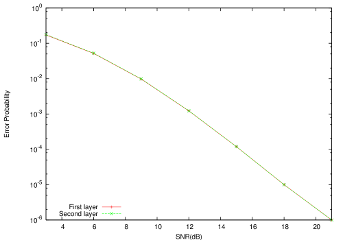
Figure 5: Error Performance of full diversity codes with $M_{t}=2$, $\nu=1$, $R_{1}=R_{2}=\frac{3}{5}$ and $d_{1}=d_{2}=4$.

From the construction of these codes, one might be tempted to conclude that the analysis for these codes is quite similar to that of cyclic codes. But the peculiar structure of the solution space i.e. the fact that given a vector in the solution space $\mathcal{B}$, not all circular shifts of the vector remain in $\mathcal{B}$, makes it difficult to analyze. The main contribution of this work is the construction of binary matrices with a particular structure which consequently characterizes the rate diversity tradeoff for the ISI channel. Note that as seen in Example 1 and 2 codes which give guaranteed diversity orders for flat fading MIMO channel, when used for transmission over ISI channel do not necessarily give the multiplicative diversity gain of $(\nu+1)$. The tools and techniques developed over here could also have independent interest in designing codes in various other wireless or distributed settings.

8 Appendix

Proof.   [of Lemma 15] We have that for some subset $S\subseteq\{1,\ldots,p\}$ there exist $\left\{\gamma_{i}\right\}_{i\in S}$ such that,

$$deg(\sum_{i\in S}\gamma_{i}\mathbf{g}^{(i)}) <\max_{i\in S}deg(\gamma_{i}\mathbf{g}^{(i)})$$ (188)

Let $t=\max_{i\in S}deg(\gamma_{i}\mathbf{g}^{(i)})$ and define $\mathcal{T}=\left\{i:deg(\gamma_{i}\mathbf{g}^{(i)})=t\right\}$. Note that we have,

$$deg(\gamma_{i}\mathbf{g}^{(i)})=deg(\alpha^{deg(\gamma_{i})}\mathbf{g}^{(i)})$$ (189)

This allows us to see that (188) implies that,

$$deg\left(\sum_{i\in\mathcal{T}}\alpha^{deg(\gamma_{i})}\mathbf{g}^{(i)}\right) <t.$$ (190)

Denote $w=\min_{i\in\mathcal{T}}(deg(\gamma_{i}))$ to be the minimum degree of $\gamma_{i}$ for $i\in\mathcal{T}$ and $k=\operatornamewithlimits{argmin}_{i\in\mathcal{T}}(deg(\gamma_{i}))$. Define $S^{\prime}=\mathcal{T}\backslash\{k\}$ where $\backslash$ is the set difference operator.

If $w=0$ then we have,

$$deg(\mathbf{g}^{(k)}+\sum_{i\in S^{\prime}}\alpha^{deg(\gamma_{i})}\mathbf{g}^{(i)}) <t=deg(\mathbf{g}^{(k)})$$

and,

$$t =deg\left(\alpha^{deg(\gamma_{i})}\mathbf{g}^{(i)}\right)\leq deg\left(\mathbf{g}^{(k)}\right)=t\quad\forall i\in S^{\prime}$$

which shows that if $w=0$, then the claim is true.

If $w\neq 0$ we can take out the common $\alpha^{w}$ factor of $\sum_{i\in\mathcal{T}}\alpha^{deg(\gamma_{i})}\mathbf{g}^{(i)}$. Then we have,

$$deg(\mathbf{g}^{(k)}+\sum_{i\in S^{\prime}}\alpha^{deg(\gamma_{i})-w}\mathbf{g}^{(i)}) <(t-w)=deg(\mathbf{g}^{(k)})$$

and,

$$t-w =deg\left(\alpha^{deg(\gamma_{i})-w}\mathbf{g}^{(i)}\right)\leq deg\left(\mathbf{g}^{(k)}\right)=t-w\quad\forall i\in S^{\prime}$$

Hence the claim is proved.  

To prove the Lemma 20 we will make use of the Cauchy Binet formula reproduced here for completeness.

Definition 22

Cauchy Binet Formula [12] Let $\mathbf{A}$ be a $m\times n$ matrix and $\mathbf{B}$ be a $n\times m$ matrix. If $S$ is a subset of $\{1,\ldots,n\}$ with $m$ elements, let $\mathbf{A}_{S}$ represent the $m\times m$ matrix whose columns are those columns of $\mathbf{A}$ that have indices from $S$. Similarly, let $\mathbf{B}_{S}$ represent the $m\times m$ matrix whose rows are those rows of $\mathbf{B}$ that have indices from $S$. The Cauchy-Binet formula then states that,

$$det(\mathbf{AB}) =\sum_{S}det(\mathbf{A}_{S})\det(\mathbf{B}_{S})$$ (191)

where the sum extends over all possible subsets $S$ of $\{1,\ldots,n\}$ with $m$ elements.

Note that the Cauchy Binet formula holds for matrices with entries from any commutative rings. Given this definition, the proof of lemma 20 proceeds as follows.

Proof.   [of Lemma 20] The matrix $\mathbf{P}$ is given by,

$$\mathbf{P} =\underbrace{\left[\begin{array}[]{c}\mathbf{g}^{(1)}\\ \mathbf{g}^{(2)}\\ \vdots\\ \mathbf{g}^{(R)}\end{array}\right]}_{\mbox{${\bf M}$}\in\Gamma^{R\times M_{t}}}\underbrace{\left[\begin{array}[]{cccc}1&\ldots&1&1\\ \xi^{2^{R-1}}&\ldots&\xi^{2}&\xi\\ (\xi^{2})^{2^{R-1}}&\ldots&(\xi^{2})^{2}&\xi^{2}\\ \vdots&&\vdots&\\ (\xi^{(M_{t}-1)})^{2^{R-1}}&\ldots&(\xi^{(M_{t}-1)})^{2}&\xi^{(M_{t}-1)}\\ \end{array}\right]}_{\mathbf{W}\in\mathbb{F}_{2^{T}}^{M_{t}\times R}}$$

Using Gaussian elimination (which can be applied over any finite field), we reduce the matrix ${\bf M}$ to its row echelon form,

$$\mathbf{\breve{Y}} =\left[\begin{array}[]{c}\breve{\mathbf{g}}^{(1)}\\ \breve{\mathbf{g}}^{(2)}\\ \vdots\\ \breve{\mathbf{g}}^{(R)}\end{array}\right]$$

where

$$deg(\breve{\mathbf{g}}^{(k)}) \leq 2^{(R-k)}\nu.$$

Note that this pivoting and reduction to a row echelon form is a full rank operation and preserves the rank of $\mathbf{P}$. Therefore,

$$det(\mathbf{P}) =Kdet\left(\mathbf{\breve{Y}}\mathbf{W}\right)$$

where $K\in\mathbb{F}_{2^{T}}$ and $K\neq 0$. Let the columns containing the pivots in $\mathbf{\breve{Y}}$ be denoted by $\tilde{S}$. Therefore by the Cauchy Binet formula, we have

$$K^{-1}det(\mathbf{P}) =det\left(\mathbf{\breve{Y}}_{\tilde{S}}\right)det\left(\mathbf{W}_{\tilde{S}}\right)+\sum_{S\neq\tilde{S}}det\left(\mathbf{\breve{Y}}_{S}\right)det\left(\mathbf{W}_{S}\right)$$ (192)

Note that for all $S$ such that $det\left(\mbox{${\bf M}$}_{S}\right)\neq 0$ the maximum coefficient of $\xi$ in $det\left(\mathbf{W}_{S}\right)$ is less than the maximum coefficient of $\xi$ in $det\left(\mathbf{W}_{\tilde{S}}\right)$ by at least $1$. Therefore,

$$deg(det\left(\mathbf{W}_{\tilde{S}}\right))-deg(det\left(\mathbf{W}_{S}\right)) \geq(2^{R}-1)(\nu+1)$$

Also note that,

$$deg(det(\mbox{${\bf M}$}_{S}))-deg(det(\mbox{${\bf M}$}_{\tilde{S}})) \leq\nu+2\nu+2^{2}\nu+\ldots+2^{R-1}\nu$$

$$=\nu(2^{R}-1)$$

Therefore,

$$deg(det\left(\mathbf{W}_{\tilde{S}}\right)det(\mbox{${\bf M}$}_{\tilde{S}}))-deg(det\left(\mathbf{W}_{S}\right)det(\mbox{${\bf M}$}_{S})) \geq(2^{R}-1)(\nu+1)-\nu(2^{R}-1)$$

$$>0$$

Therefore by the linear independence of $\{1,\alpha,\ldots,\alpha^{T-1}\}$ we can conclude that there exists a term in $det\left(\mathbf{W}_{\tilde{S}}\right)det(\mbox{${\bf M}$}_{\tilde{S}})$ with a power of $\alpha$ which in not canceled by any other term in the equation (192). Therefore we conclude that $K^{-1}det(\mathbf{P})\neq 0$ implying $det(\mathbf{P})\neq 0$. Hence proved.

References

- [1] A. R. Calderbank, S. N. Diggavi and N. Al-Dhahir. Space-Time Signaling based on Kerdock and Delsarte-Goethals Codes. IEEE International Conference on Communications (ICC), pp 483 - 487, Paris, June 2004.
- [2] S. N. Diggavi, N. Al-Dhahir, and A. R. Calderbank, Diversity embedding in multiple antenna communications, advances in network information theory. DIMACS Series in Discrete Mathematics and Theoretical Computer Science, pages 285-301, 2004.
- [3] S. N. Diggavi and D. Tse, Fundamental Limits of Diversity-Embedded Codes over Fading Channels, IEEE International Symposium on Information Theory (ISIT), pp 510–514. September, 2005.
- [4] S. N. Diggavi and D. Tse, On opportunistic codes and broadcast codes with degraded message sets, IEEE Information Theory Workshop (ITW), pp 227–231, March, 2006.
- [5] S. N. Diggavi, S. Dusad, A. R. Calderbank, N. Al-Dhahir, On Diversity Embedded codes, Proceedings of Allerton Conference on Communication, Control, and Computing, Illinois, September 2005.
- [6] S. N. Diggavi, A. R. Calderbank, S. Dusad and N. Al-Dhahir, Diversity embedded space-time codes, preprint, submitted to IEEE Transactions on Information Theory, 2006
- [7] S. Dusad and S N. Diggavi, On successive refinement of diversity for fading ISI channels, Proceedings of Allerton Conference on Communication, Control, and Computing, Illinois, September 2006.
- [8] E. Gabidulin, Theory of codes with maximum rank distance. Probl. Per. Inform., 21:3–16, Jan/March 1985.
- [9] H. E. Gamal, A. R. Hammons, Y. Liu, M. P. Fitz, O. Y. Takeshita, On the Design of Space-Time and Space-Frequency Codes for MIMO Frequency Selective Fading Channels, IEEE Transactions on Information Theory, 49(9):2277–2291, September 2003.
- [10] J-C. Guey, M. P. Fitz, M. R. Bell, and W-Y. Kuo, Signal design for transmitter diversity wireless communication systems over Rayleigh fading channels. IEEE Transactions on Communications, 47(4):527–537, April 1999.
- [11] A. R. Hammons, Jr., H. El-Gamal, On the theory of space-time codes for PSK modulation, IEEE Transactions on Information Theory, Vol 46, No. 2, pp 524–542, March 2000.
- [12] R. Horn and C. Johnson Matrix Analysis. Cambridge University Press, 1990
- [13] R. Lidl and H. Niederreiter Finite Fields. Cambridge University Press, 1997
- [14] H. F. Lu and P. V. Kumar, Rate-diversity trade-off of space-time codes with fixed alphabet and optimal constructions for PSK modulation, IEEE Transactions on Information Theory, 49(10):2747–2752, October 2003.
- [15] H. F. Lu and P. V. Kumar, A unified construction of space-time codes with optimal rate-diversity tradeoff, IEEE Transactions on Information Theory, 51(5):1709–1730, May 2005.
- [16] R. J. McEliece Finite Fields for Computer Scientists and Engineers. Kluwer Academic Publishers, 2003
- [17] W. Su, Z. Safar, M. Olfat, R. Liu, Obtaining full-diversity space-frequency codes from space-time codes via mapping IEEE Transactions on Signal Processing, 51(11):2905–2916, November 2003.
- [18] V. Tarokh, N. Seshadri, and A.R. Calderbank. Space-time codes for high data rate wireless communications: Performance criterion and code construction. IEEE Transactions on Information Theory, 44(2):744–765, March 1998.
- [19] D. N. C. Tse and P. Viswanath, Fundamentals of Wireless Communication,Cambridge University Press, 2005
- [20] L. Washington Introduction to cyclotomic fields, Springer Verlag, 2nd edition June 1997.