A new twist on Lorenz links

Abstract

Twisted torus links are given by twisting a subset of strands on a closed braid representative of a torus link. T–links are a natural generalization, given by repeated positive twisting. We establish a one-to-one correspondence between positive braid representatives of Lorenz links and T–links, so Lorenz links and T–links coincide. Using this correspondence, we identify over half of the simplest hyperbolic knots as Lorenz knots. We show that both hyperbolic volume and the Mahler measure of Jones polynomials are bounded for infinite collections of hyperbolic Lorenz links. The correspondence provides unexpected symmetries for both Lorenz links and T-links, and establishes many new results for T-links, including new braid index formulas.

1 Introduction

The Lorenz differential equations [20] have become well-known as the prototypical chaotic dynamical system with a “strange attractor” (see [27], and references therein). A periodic orbit in the flow on $\mathbb{R}^{3}$ determined by the Lorenz equations is a closed curve in $\mathbb{R}^{3}$, which defines a Lorenz knot. Lorenz knots contain many known classes of knots, but the complete classification of Lorenz knots remains open: What types of knots can occur?

Guckenheimer and Williams introduced the Lorenz template, also called the geometric Lorenz attractor, which is an embedded branched surface in $\mathbb{R}^{3}$ with a semi-flow. Later, Tucker [26] rigorously justified this geometric model for Lorenz’s original parameters. Using this model, closed orbits in the Lorenz dynamical system have been studied combinatorially with symbolic dynamics on the template. Indeed, the Lorenz template (see Figure 1(a))

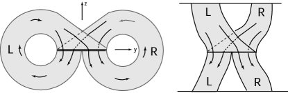
Figure 1: (a)The Lorenz template.  (b)The Lorenz braid template

can be viewed as a limit of its periodic orbits, a kind of link with infinitely many knotted and linked components. Starting with the template, Birman and Williams [3] initiated the systematic study of Lorenz knots. They proved that infinitely many distinct knot types occur, including all torus knots and certain cables on torus knots.

Recently, Ghys [16] established a startling connection with the periodic orbits in the geodesic flow on the modular surface, which are in bijection with hyperbolic elements in ${\rm PSL}(2,\mathbb{Z})$. Any hyperbolic matrix $A\in{\rm PSL}(2,\mathbb{Z})$ defines a periodic orbit, which Ghys called a modular knot, in the associated modular flow on the complement of the trefoil knot in $S^{3}$. Ghys proved that isotopy classes of Lorenz knots and modular knots coincide. His proof relies on ingenious deformations that ultimately show that periodic orbits of the modular flow can be smoothly isotoped onto the Lorenz template embedded in ${\rm PSL}(2,\mathbb{R})/{\rm PSL}(2,\mathbb{Z})$. (See also [18], a survey article on this work with breathtaking images.)

We define Lorenz links to be all links on the Lorenz template; i.e., all finite sublinks of the ‘infinite link’ above, a definition that coincides with Ghys’ modular links [16, 17]. This definition is broader than the one used in [3], which excluded any link with a parallel cable around any component. Thus, Lorenz links are precisely all links as in [3], together with any parallel push-offs on the Lorenz template of any sublinks. Lorenz knots are the same in both definitions, but Lorenz links include, for example, all $(n,n)$–torus links, which are excluded from links in [3] for $n\geq 4$. Lorenz braids are all braids on the braid template.

We define T-links as follows. The link defined by the closure of the braid $(\sigma_{1}\cdots\sigma_{r-1})^{s}$ is a torus link T$(r,s)$. For $2\leq r_{1}\leq\ldots\leq r_{k},\ \ 0<s_{i},\ \ i=1,\dots,k$, let T$((r_{1},s_{1}),\ldots,(r_{k},s_{k}))$ be the link defined by the closure of the following braid, all of whose crossings are positive:

$$\mathbb{T}=(\sigma_{1}\sigma_{2}\cdots\sigma_{r_{1}-1})^{s_{1}}(\sigma_{1}\sigma_{2}\cdots\sigma_{r_{2}-1})^{s_{2}}\cdots(\sigma_{1}\sigma_{2}\cdots\sigma_{r_{k}-1})^{s_{k}}.$$ (1)

We call $\mathbb{T}$ a T–braid, and refer to the link $\mathcal{T}$ that its closure defines as a T-link. See Figure 2 for examples (note that braids are oriented anticlockwise).

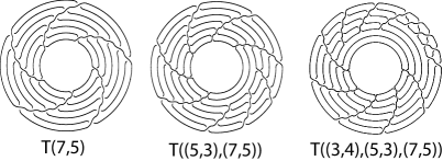
Figure 2: Examples of T-links

Note that T–knots, in the case $k=2$, are both more general and less general than the twisted torus knots studied in [4, 7]. In those references, twisted torus knots are obtained by performing $s$ full twists on $r$ strands of a $(p,q)$–torus knot. This means that $s_{1}$ is a multiple of $r_{1}$, which we do not require in general. On the other hand, in those references the twists need not be positive.

In this paper, in Theorem 1 we establish the following one-to-one correspondence: Every Lorenz link is a T–link, and every T–link is a Lorenz link. Among many interesting consequences for both T–links and Lorenz links, this correspondence suggests a fertile new area for investigation: the hyperbolic geometry of Lorenz knot complements.

To set up the background, and explain what we learned, recall that modern knot theory originated with efforts to tabulate knot types. Starting at the end of the 19th century, tables of knots ordered by their minimum crossing number were constructed. The early tables went through 9 and then 10 crossings, and were constructed entirely by hand. Roughly 100 years later that project was carried as far as good sense dictated, when two separate teams, working independently and making extensive use of modern computers, tabulated all distinct prime knots of at most 16 crossings, learning in the process that there there are 1,701,936 of them, now available using the computer program Knotscape. These ‘knot tables’ have served for many years as a rich set of examples. The use of minimum crossing number as a measure of complexity may actually have added to the usefulness of the tables, because crossing number has limited geometric meaning, so the tabulated knots serve in some sense as a random collection.

Ghys and Leys [18] had stressed the scarcity of Lorenz knots in the knot tables. In particular, Ghys had obtained data which showed that among the 1,701,936 prime knots with 16 crossings or fewer, only 20 appear as Lorenz knots, with only 7 of those non-torus knots. It would seem that Lorenz knots are a very strange and unfamiliar collection.

The study of hyperbolic 3-manifolds, and in particular hyperbolic knot complements, is a focal point for much recent work in 3-manifold topology. Thurston showed that a knot is hyperbolic if it is neither a torus knot nor a satellite knot. His theorems changed the focus of knot theory from the properties of diagrams to the geometry of the complementary space. Ideal tetrahedra are the natural building blocks for constructing hyperbolic 3-manifolds, and ideal triangulations can be studied using the computer program SnapPea. There are 6075 noncompact hyperbolic 3-manifolds that can be obtained by gluing the faces of at most seven ideal tetrahedra [5]. For a hyperbolic knot, the minimum number of ideal tetrahedra required to construct its complement is a natural measure of its geometric complexity.

In [4, 7], it was discovered that twisted torus knots occur frequently in the list of “simplest hyperbolic knots,” which are knots whose complements are in the census of hyperbolic manifolds with seven or fewer tetrahedra. Since those twisted torus knots were not all positive, we collected new data to determine how many were Lorenz knots. By the correspondence in Theorem 1,

• Of the 201 simplest hyperbolic knots, at least 107 are Lorenz knots.

The number 107 could be too small because, among the remaining 94 knots, we were unable to decide whether five of them are or are not Lorenz. Many knots in the census had already been identified as positive twisted torus knots, though their diagrams did not in any way suggest the Lorenz template. Lorenz braids for the known Lorenz knots in the census are provided in a table in Section 5.

The data in the census suggests a very interesting question:

Question 1

Why are so many geometrically simple knots Lorenz knots?

The heart of the proof of Theorem 1 is simply that the links in question are all positive, and happen to have two very different kinds of closed positive braid representations: as Lorenz braids on the one hand, and as T-braids on the other hand. Theorem 1 has immediate consequences for T-links. Corollary 1 asserts that all of the properties that were established in [3] for Lorenz links apply now to T-links, and in particular to positive twisted torus links. For example, T-links are prime, fibered, non-amphicheiral, and have positive signature.

Another easy consequence for Lorenz links, which was useful for recognizing Lorenz knots in the census, is Corollary 2: Every Lorenz link $\mathcal{L}$ has finitely many representations as a Lorenz braid, up to trivial stabilizations.

Further consequences depend on the observation that the correspondence in Theorem 1 implies certain new symmetries. Corollary 3 applies a somewhat subtle symmetry of T-links, which generalizes the well-known but not uninteresting fact that T$(r,s)=$ T$(s,r)$ to Lorenz links. Going the other way, there is an obvious symmetry of Lorenz braids by ‘turning over the template’, which provides a non-obvious involution for T–braids. The involution exchanges the total numbers of strands that are being twisted for numbers of over-passes in the twisted braid. See Corollary 4. In the special case of positive twisted torus links, it asserts that T$((r_{1},s_{1}),(r_{2},s_{2}))$ and T$((s_{2},r_{2}-r_{1}),(s_{1}+s_{2},r_{1}))$ have the same link type.

This symmetry, generalized to all T-links below, is quite interesting in its own regard, and it also enables us to establish new properties of Lorenz links. It is a well-known open problem, with many related important conjectures, to find the precise relationship between the hyperbolic volume and the Jones polynomial of a knot. Using Theorem 1, the duality of Corollary 4, Thurston’s Dehn surgery theorem [25], and results in [6], we are able to show that both hyperbolic volume and Mahler measure of Jones polynomials are bounded for very broadly defined infinite families of Lorenz links.

Let $N>0$. Let $\mathcal{L}$ be a Lorenz link or T–link satisfying any one of the following conditions: The Lorenz braid of $\mathcal{L}$ has at most $N$ over-crossing (or under-crossing) strands, or equivalently, the T–braid of $\mathcal{L}$ has at most $N$ strands (i.e. $r_{k}\leq N$), or at most $N$ over-passes (i.e. $s_{1}+\ldots+s_{k}\leq N$). Corollaries 5 and 6 assert:

1. If $\mathcal{L}$ is hyperbolic, its hyperbolic volume is bounded by a constant that depends only on $N$.

2. The Mahler measure of the Jones polynomial of $\mathcal{L}$ is bounded by a constant that depends only on $N$.

The Jones polynomials of Lorenz links are very atypical, sparse with small nonzero coefficients, compared with other links of equal crossing number. Pierre Dehornoy [10] assembled a great deal of data, but the polynomials were too complicated to pin down precisely. Corollary 7 summarizes the relevant known results about the degrees of the Jones, HOMFLY and Alexander polynomials of links that can be represented as closed positive braids, and so about Lorenz links.

Continuing our quick review of the paper, we briefly discuss braid representations of Lorenz links at minimal braid index. It is known that the braid index of a Lorenz knot is its trip number, a concept that was first encountered in the study of Lorenz knots from the point of view of symbolic dynamics (see [3]). In view of the 1-1 correspondence in Theorem 1, an immediate consequence is that the braid index of each corresponding T–link is also known. Nevertheless, a problem arises: If $\mathcal{T}$ is a T–link, the trip number of its Lorenz companion $\mathcal{L}$ is not easily computed from the defining parameters for the T–link. In Corollary 8, we give an explicit formula for computing it directly from the sequence of integer pairs $((r_{1},s_{1}),\dots,(r_{k},s_{k}))$ that define $\mathcal{T}$.

In $\S$4, we prove Theorem 2, which establishes for any Lorenz link $\mathcal{L}$, a correspondence between its Lorenz braid representations and particular factorizations of braid words in the braid group $B_{t}$, where $t$ is the minimal braid index of $\mathcal{L}$. This theorem is a strong form of Proposition 5.1 of [3], and is interesting because it applies to T–links as well as to Lorenz links.

We return to the hyperbolicity question: When is a Lorenz link hyperbolic? We could not answer that question, but as a starter Corollary 9 gives a fast algorithm to decide when a Lorenz link is a torus link.

Here is a guide to this paper. In $\S$2 we set up our notation and prove a basic lemma about the repeated removal of trivial loops in a Lorenz braid. The lemma will be used in the proofs of Theorems 1 and 2. In $\S$3, we state and prove Theorem 1 and Corollaries 1–8. In $\S$4 we prove Theorem 2 and Corollary 9. In $\S$5, we discuss and provide Lorenz data for the simplest hyperbolic knots. Open questions are scattered throughout the paper.

Acknowledgments We thank the two referees of an early version of this paper for their thoughtful and constructive comments. We thank Slavik Jablan for sharing with us the list of Lorenz knots up to 49 crossings, and verifying for us that certain simplest hyperbolic knots are not on this list, as discussed in Section 5. We thank Volker Gebhardt for sharing his program to draw closed braids, which was used to make Figure 2. We thank Pierre Dehornoy, Etienne Ghys, Juan Gonzalez-Meneses, Slavik Jablan, Michael Sullivan, and Robert Williams for carefully answering our questions.

2 Preliminaries

We defined a Lorenz link to be any finite collection of closed orbits on the Lorenz template, which supports a semiflow. The template is a branched 2-manifold embedded in $\mathbb{R}^{3}$, as illustrated in Figure 1. In the right sketch, the Lorenz template has been cut open to give a related template for Lorenz braids, which inherit an orientation from the template, top to bottom. The crossings in Figure 3 will be called positive crossings. Although this convention is opposite to the usual one in knot theory, it matches [3] and has often appeared in the related literature, so we continue to use it now.

Example 1

Figure 3 gives an example of a Lorenz braid. It becomes a Lorenz knot after connecting the strands as in a closed braid, on the template. This example will be used throughout the paper to illustrate our ideas, so Figure 3 contains features that will be explained later.

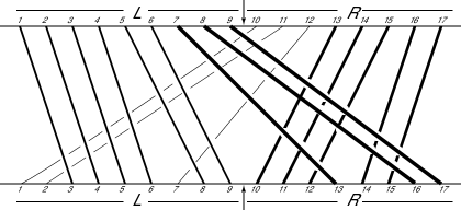
Figure 3: $\vec{d}_{L}=\langle 2,2,2,2,3,3,6,8,8\rangle=\langle 2^{4},3^{2},6^{1},8^{2}\rangle$

The Lorenz braid $\mathbb{L}$ is determined entirely by its permutation, because any two strands cross at most once. In a Lorenz braid two overcrossing (resp. undercrossing) strands never intersect, so the permutation associated to the overcrossing strands uniquely determines the rest of the permutation. Therefore, $\mathbb{L}$ is determined by just the permutation associated to its overcrossing strands.

Assume there are $p>1$ overcrossing strands. On each overcrossing strand the position of the endpoint will always be bigger than that of the initial point. Suppose the $i^{\rm th}$ strand begins at $i$ and ends at $i+d_{i}$. Since two overcrossing strands never cross, we have the following sequence of positive integers:

$$d_{1}\leq d_{2}\leq\cdots\leq d_{p-1}\leq d_{p}$$

Lorenz braids that have unknotted closure were classified in Corollary 5.3 of [3]. Excluding the two trivial loops that are parallel to the two boundary components, it was proved that a Lorenz knot is unknotted if and only if the following condition holds:

$$i+d_{i}>p\quad{\rm if\ and\ only\ if}\quad i=p$$

Since $1\leq d_{1}\leq d_{2}\leq\cdots\leq d_{p}$, it follows that $d_{i}=1$ for every $i\leq p-1$. But $d_{p}$ can be $1,2,3,\dots$, and these are the only ways to obtain the unknot.

In view of this classification, we can make two assumptions: (i) $2\leq d_{1}$ and (ii) $d_{p-1}=d_{p}$. Otherwise, if $d_{1}=1$ then $\mathbb{L}=\sigma_{1}\mathbb{L}^{\prime}$ for a Lorenz braid $\mathbb{L}^{\prime}$ on the last $n-1$ strands, so that $\mathbb{L}$ can be trivially destabilized on its left side. We get similarly trivial destabilizations on the right if $d_{p-1}<d_{p}$. As we have seen, the only closed orbits omitted by making these assumptions are the Lorenz unknots.

We collect this data in the following vector (see [3]):

$$\vec{d}_{L}=\langle d_{1},\dots,d_{p}\rangle,\quad 2\leq d_{1},\ d_{p-1}=d_{p},\ {\rm and\ each}\ d_{i}\leq d_{i+1}$$ (2)

The vector $\vec{d}_{L}$ determines the positions of the L (overcrossing) strands. The R (undercrossing) strands fill in the remaining positions, in such a way that all crossings are L-strands crossing over R-strands. In Figure 3, the arrows separate the left and right strands. Each $d_{i}$ with $i=1,\dots,p$ is the difference between the initial and final positions of the $i^{\rm{th}}$ overcrossing strand. The integer $d_{i}$ is also the number of strands that pass under the $i^{\rm{th}}$ braid strand. The vector $\vec{d}_{L}$ determines a closed braid $\mathbb{L}$ on $n=(p+d_{p})$ strands, which we call the Lorenz braid representation of the Lorenz link $\cal L$. All non-trivial Lorenz links arise in this way.

The overcrossing strands travel in groups of parallel strands, which are strands of the same slope, or equivalently strands whose associated $d_{i}$’s coincide. If $d_{\mu_{j}}=d_{\mu_{j}+1}=\cdots=d_{\mu_{j}+s_{j}-1}$, where $s_{j}$ is the number of strands in the $j^{\rm{th}}$ group, then let $r_{j}=d_{\mu_{j}}$. Thus, we can write $\vec{d}_{L}$ in the form:

$$\vec{d}_{L}=\langle d_{\mu_{1}}^{s_{1}},\dots,d_{\mu_{k}}^{s_{k}}\rangle=\langle r_{1}^{s_{1}},\dots,r_{k}^{s_{k}}\rangle,\ \ 1\leq s_{i},\ \ 2\leq r_{1},s_{k},\ \ {\rm and}\ \ r_{i}<r_{i+1}.$$ (3)

where $r_{i}^{s_{i}}$ means $r_{i},\ldots,r_{i}$ repeated $s_{i}$ times. Note that

$$p=s_{1}+\cdots+s_{k},\quad d_{1}=r_{1},\quad d_{p}=r_{k}$$

The trip number $t$ of a Lorenz link $\mathcal{L}$ is given by

$$t=\#\{\ i\ |\ i+d_{i}>p\ {\rm where}\ 1\leq i\leq p\ \}$$ (4)

The trip number is the minimum braid index of $\mathcal{L}$, a fact which was conjectured in [3] and proved in [14].

In Example 1, $\langle 2,2,2,2,3,3,6,8,8\rangle=\langle 2^{4},3^{2},6^{1},8^{2}\rangle$. Thus, $p=9,\ k=4,\ r_{k}=8$, and $n=p+r_{k}=17$ is the braid index of $\mathbb{L}$. The trip number $t=3$ is the braid index of the Lorenz link given by the closure of $\mathbb{L}$.

Our first new result is little more than a careful examination of the proof of Theorem 5.1 of [3]. This lemma will be used in the proofs of Theorems 1 and 2 of this paper.

Lemma 1

Let $\mathbb{L}$ be a Lorenz braid defined by $\vec{d}_{L}=\langle r_{1}^{s_{1}},\dots,r_{k}^{s_{k}}\rangle=\langle d_{1},\dots,d_{p}\rangle$, so $\mathbb{L}$ is a braid on $p+r_{k}$ strands. Then there is a sequence of closed positive braids:

$$\mathbb{L}=\mathbb{L}_{0}\to\mathbb{L}_{1}\to\mathbb{L}_{2}\to\cdots\to\mathbb{L}_{p}\to\cdots\to\mathbb{L}_{p+r_{k}-t}$$

where each $\mathbb{L}_{i+1}$ is obtained from $\mathbb{L}_{i}$ by single move that reduces the braid index and also the crossing number by $1$. Each $\mathbb{L}_{i}$ represents the same Lorenz link $\mathcal{L}$. The intermediate braid $\mathbb{L}_{p}$ in the sequence has $r_{k}$ strands, and the final braid $\mathbb{L}_{p+r_{k}-t}$ has $t$ strands, which is the minimum braid index of $\mathcal{L}$.

Proof:  We will find the required Markov sequence by using a geometric trick that was introduced in [3].

The letters $1,2,\dots,p$ in a Lorenz permutation are said to be in the left or L-group, and the letters $p+1,\dots,p+r_{k}$ are in the right or R-group. Each strand in a Lorenz braid begins and ends at a point which is either in L or in R, therefore the strands divide naturally into 4 groups: strands of type LL, LR, RL and RR, where strands of type LL (resp. LR) begin on L and end on L (resp. R), and similarly for types RL and RR. In the example in Figure 3, those of type LR are the thickest, with those of type RR, LL and RL each a little thinner than their predecessors.

By definition of the trip number $t$ in (4), there are $p-t,\ t,\ t$ and $r_{k}-t$ strands of type LL,LR,RL and RR respectively. In sketch (i) of Figure 4 we have cut open the Lorenz template, snipping it open between two orbits, as was done in [3], so that the template itself divides naturally into bands of type LL,LR,RL and RR.

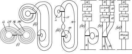
Figure 4: Cutting open the Lorenz template

In sketch (ii), we stretched out the band that contains all of the strands of type LR, and in sketch (iii) we uncoiled that band, introducing a full twist into the $t$ strands of type LR. This uncoiling can be regarded as having been done one strand at a time, and when we think of it that way, it becomes a sequence of $t$ moves, each reducing the braid index by 1. Observe that when we ‘uncoil’ the outermost arc (and the ones that follow too), we trade one arc in the braid $\mathbb{L}_{i}$ for a ‘shorter’ arc in the braid $\mathbb{L}_{i+1}$, reducing the braid index by 1. This process has been repeated $t$ times in the passage from sketch (ii) to sketch (iii), because there are $t$ strands in the LR braid. The uncoiling takes positive braids to positive braids, although the property of being a Lorenz braid is not preserved. After the $t$ Markov moves illustrated in the passage to sketch (iii), the braid index will have been reduced from $p+r_{k}$ to $p+r_{k}-t$.

We turn our attention to the LL subbraid in sketch (iii), which has $p-t$ strands. The strands of type RL and of type LR both have $t$ strands. From this it follows that when the LL band is uncoiled, we obtain a subbraid on $t$ strands that joins the RL subbraid to the LR subbraid, as illustrated in sketch (iv) of Figure 4. Figure 5, illustrates via an example the uncoiling that leads to the LL braid.

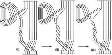
Figure 5: Uncoiling the LL braid: an example

The example shown in Figure 5 is the Lorenz braid from Example 1, shown in Figure 3. It’s a rather simple example because the trip number $t=3$. Sketch (i) in Figure 5 corresponds to sketch (iii) in Figure 4. Sketches (ii) and (iii) of Figure 5 show two destabilizations, and correspond to two steps in the passage from sketch (iii) to sketch (iv) of Figure 4.

In the LL braid, we uncoil the $i^{th}$ strand, which is the outer coiled strand in the leftmost sketch in Figure 5. Let $\gamma_{i}$ be this outer arc running clockwise and crossing over three strands in the sketch. If $\pi$ is the permutation associated to the Lorenz braid $\mathbb{L}$, say $\gamma_{i}(0)$ corresponds to the bottom endpoint $i$, $\gamma_{i}(1/2)$ corresponds to the top endpoint $i$, and $\gamma_{i}(1)$ corresponds to $\pi(i)=i+d_{i}$. Therefore, in the middle sketch of Figure 5, $\gamma_{i}$ is replaced by an arc that contributes $(\sigma_{1}\sigma_{2}\cdots\sigma_{d_{i}-1})$ to the LL braid. Continuing in this way, the LL braid determines $\prod_{i=1}^{i=p-t}(\sigma_{1}\sigma_{2}\cdots\sigma_{d_{i}-1})$.

We return to Figure 4. There are $p-t$ strands in the LL braid, so there are $p-t$ strands that are uncoiled in sketch (iv). The braid index will go down from $(p+r_{k}-t)$, in sketch (iii), to $(p+r_{k}-t)-(p-t)=r_{k}$ in sketch (iv). In sketch (v) we have cut open the right coil, exhibiting the braid template for the $r_{k}$–braid to be studied in Theorem 1. This braid was not considered in [3].

The final braid in the sequence is illustrated in sketch (vi). It is obtained from the braid in sketch (iv) by uncoiling the RR braid. It was proved in [3] to have braid index $t$, where $t$ is the trip number. We will study it further in $\S$4.

Each braid $\mathbb{L}_{i+1}$ in the sequence that we just described has braid index one less than that of its predecessor $\mathbb{L}_{i}$. To prove the assertion about crossing number, observe that since each $\mathbb{L}_{i}$ is a positive braid, an Euler characteristic count shows that

$$2g(\mathcal{L})=c(\mathbb{L}_{i})-n(\mathbb{L}_{i})-\mu(\mathcal{L})+2,$$

where $c$ is the crossing number of the positive braid $\mathbb{L}_{i}$, $n$ is its braid index, $g$ is the genus, and $\mu$ is the number of components of $\mathcal{L}$. But then $c(\mathbb{L}_{i})-n(\mathbb{L}_{i})$ is a topological invariant of $\mathcal{L}$, so when $n$ is reduced $c$ must be reduced too. This completes the proof of Lemma 1. $\blacksquare$

3 Lorenz links and T-links

T-links were defined in $\S$1 above.

Theorem 1

Every Lorenz link is a T–link, and every T–link is a Lorenz link.

Precisely, if a link $\mathcal{L}$ is represented by a Lorenz braid $\mathbb{L}$ on $p+r_{k}$ strands with $\vec{d}_{L}=\langle r_{1}^{s_{1}},\dots,r_{k}^{s_{k}}\rangle$, then $\mathcal{L}$ also has an $r_{k}$–braid representation $\mathbb{T}$, given in (1), which exhibits it as a T–link. Moreover, every T–link arises in this way from some Lorenz link.

Proof:  We begin by introducing convenient notation. Let $v,w$ be positive integers with $v<w$. Let $[v,w]=\sigma_{v}\sigma_{v+1}\cdots\sigma_{w-1}$ and let $[w,v]=\sigma_{w-1}\cdots\sigma_{v+1}\sigma_{v}$. If $u<v<w$, we have a very simple product rule:

$$[u,v][v,w]=[u,w]$$ (5)

In the braid group $B_{n}$, an index shift relation holds:

$$(\sigma_{1}\sigma_{2}\dots\sigma_{k-1}\sigma_{k})(\sigma_{j})=(\sigma_{j+1})(\sigma_{1}\sigma_{2}\dots\sigma_{k-1}\sigma_{k}),\ \ j=1,2,\dots,k-1$$

The index shift relation can be expressed in our new notation as:

$$[1,w][u,v]=[u+1,v+1][1,w]\ \ {\rm if}\ v<w$$ (6)

We now study the braids in sketch (v) of Figure 4 in detail. In the proof of Lemma 1, which was based upon Figure 4, we produced a Markov sequence from our original braid $\mathbb{L}\in B_{p+r_{k}}$ to a braid $\mathbb{L}_{p}\in B_{r_{k}}$. It is clear from sketch (v) of Figure 4 that $\mathbb{L}_{p}$ is a product of braids $\mathbb{XYZ}\in B_{r_{k}}$, where $\mathbb{X}$ comes from the LL braid, $\mathbb{Y}$ from the LR braid, and $\mathbb{Z}$ from the RL and RR braids. Both $\mathbb{X}$ and $\mathbb{Y}$ use only the first $t$ strands, their remaining $r_{k}-t$ strands being the identity braid, but $\mathbb{Z}$ uses all $r_{k}$ strands.

In the proof of Lemma 1, we learned that the braid word that describes $\mathbb{X}$ is a product of the form:

$$\mathbb{X}=\prod_{i=1}^{p-t}(\sigma_{1}\sigma_{2}\cdots\sigma_{d_{i}-1})=\prod_{i=1}^{p-t}\;[1,d_{i}]$$ (7)

We will identify the braid $\mathbb{YZ}$ that is associated to the LR, RR and RL subbraids in Figure 4. From sketch (iii) of Figure 4, one sees immediately that $\mathbb{Y}=[1,t]^{t}$. Let $\mathbb{Z}_{t}$ be the braid on $r_{k}$ strands that is created when the strand that begins at position $t$ and ends in position $(t+r_{k})-t=r_{k}$ crosses over all the intermediate strands, with every strand that is not crossed remaining fixed. So $\mathbb{Z}_{t}=[t,r_{k}]$. Let $\mathbb{Z}_{t-i}$ be the braid that is associated to the strand that begins at $t-i$, where $i=0,1,\dots,t-1.$ This strand crosses over all the intermediate strands, but all strands that are not crossed remain fixed. Therefore

$$\mathbb{Z}_{t-i}=[t-i,t-i+d_{p-i}-t]=[t-i,d_{p-i}-i].$$

Our next claim is the key to the proof of Theorem 1:

Let $\mathbb{Y}=[1,t]^{t}$ and let $\mathbb{Z}=\mathbb{Z}_{t}\mathbb{Z}_{t-1}\cdots\mathbb{Z}_{1}$. We claim:

$$\mathbb{Y}\mathbb{Z}=[1,d_{p-t+1}][1,d_{p-t+2}]\cdots[1,d_{p}]$$ (8)

We will prove (8) by induction on $i$, where $i=0,1,\dots,t-1$. Let $\mathbb{Y}_{i}=[1,t]^{i+1}$, and let $\mathbb{Z}(i)=\mathbb{Z}_{t}\cdots\mathbb{Z}_{t-i}$. If $i=0$, we have: $\mathbb{Y}_{0}\mathbb{Z}(0)=\mathbb{Y}_{0}\mathbb{Z}_{t}=[1,t][t,d_{p}]=[1,d_{p}]$, so the induction begins. Choose any $i$ with $0<i<t$ and assume, inductively, that

$$\mathbb{Y}_{i}\mathbb{Z}_{t}\mathbb{Z}_{t-1}\dots\mathbb{Z}_{t-i}=[1,d_{p-i}]\cdots[1,d_{p-1}][1,d_{p}].$$

Since $\mathbb{Z}_{t-(i+1)}=[t-(i+1),d_{p-(i+1)}-(i+1)]$, by our induction hypothesis,

$$\mathbb{Y}_{i+1}\mathbb{Z}_{t}\dots\mathbb{Z}_{t-(i+1)}=[1,t][1,d_{p-i}]\cdots[1,d_{p}][t-(i+1),d_{p-(i+1)}-(i+1)]$$ (9)

We must prove that the right-hand side of (9) equals $[1,d_{p-(i+1)})]\cdots[1,d_{p}]$. This exercise reveals some subtle consequences of the braid relations. The product rule (5) and index shift relation (6) will play crucial roles. We claim that, as a consequence of (6), the factor $[t-(i+1),d_{p-i}-(i+1)]$ on the right in (9) can be shifted to the left, past all but one of the brackets on its left, changing its name as it does so. The reasons are:

• By our basic definition of the $d_{i}$’s, we know $d_{p-i}\leq d_{p-i-j}$ for all $j>0$.

• Every strand of type LR crosses over all strands of type RL. Since there are $t$ strands of type RL, we conclude that $t<d_{p-t+1}\leq d_{p-i}$ for all $i=0,1,\dots,t-1$.

These imply that (6) is applicable $i+1$ times, so that (9) simplifies as follows:

$$\mathbb{Y}_{i+1}\mathbb{Z}_{t}\dots\mathbb{Z}_{t-(i+1)} = [1,t][1,d_{p-i}]\cdots[1,d_{p-1}][1,d_{p}][t-(i+1),d_{p-i}-(i+1)]$$ (10)

$$= [1,t][1,d_{p-i}]\cdots[1,d_{p-1}][t-i,d_{p-i}-i][1,d_{p}]=\cdots=$$

$$= [1,t][t,d_{p-(i+1)})][1,d_{p-i}]\cdots[1,d_{p-1}][1,d_{p}]$$

Finally, we use (5) to combine the two leftmost terms in (10), obtaining:

$$=[1,d_{p-(i+1)}][1,d_{p-i}]\cdots[1,d_{p-1}][1,d_{p}]$$

This is the desired expression, so (8) is proved.

Let’s put together the expression for $\mathbb{X}$ in (7) and $\mathbb{YZ}$ in (8). After collecting like terms in the previous expression, we obtain:

$$\mathbb{XYZ} = [1,d_{1}][1,d_{2}]\cdots[1,d_{p-t}][1,d_{p-t+1}]\cdots[1,d_{p}]$$ (11)

$$= [1,d_{1}][1,d_{2}]\cdots[1,d_{p}]$$

$$= [1,r_{1}]^{s_{1}}\cdots[1,r_{k}]^{s_{k}}=(\sigma_{1}\cdots\sigma_{r_{1}-1})^{s_{1}}\cdots(\sigma_{1}\cdots\sigma_{r_{k}-1})^{s_{k}}$$ (12)

where, in the passage (11) $\to$ (12), we have collected those terms for which successive entries $d_{i}$ and $d_{i+1}$ coincide, as in the passage (2) $\to$ (3). But (12) is precisely what we claim in Theorem 1.

The only remaining question is whether every T–braid is obtained from some Lorenz link. Suppose we are given an arbitrary T–braid $\mathbb{T}$, whose closure is the T–link T$((r_{1},s_{1}),\ldots,(r_{k},s_{k}))$. Let $\vec{d}_{L}=\langle r_{1}^{s_{1}},\dots,r_{k}^{s_{k}}\rangle$, which determines a Lorenz braid $\mathbb{L}$. By the proof above, $\mathbb{L}$ is braid-equivalent to $\mathbb{T}$. This completes the proof of Theorem 1. $\blacksquare$

There are many consequences of Theorem 1. We can immediately establish many new properties for T–links:

Corollary 1

The following properties of Lorenz links are also satisfied by all T-links, and so in particular by positive twisted torus links.

• T–links are prime.

• T–links are fibered. Their genus $g$ is given by the formula $2g=c-n+2-\mu$, where $n$ is the braid index of any positive braid representation, $c$ is the crossing number of same, and $\mu$ is the number of components.

• T–links are non-amphicheiral and have positive signature.

Proof:  Property (i) was proved by Williams in [28]. His proof is interesting for us, because it illustrates the non-triviality of Theorem 1. Williams used the fact that all Lorenz links embed in the Lorenz template, and if a Lorenz link was not prime then a splitting 2-sphere would have to intersect the template in a way that he shows is impossible. Without the structure provided by the template, it seems very difficult to establish this result for T–links. Properties (ii) and (iii) were established in [3] for Lorenz links. By Theorem 1, they also hold for T-links. $\blacksquare$

Theorem 1 provides an easy proof that there are finitely many non-trivial Lorenz braid representations for any Lorenz link:

Corollary 2

Every Lorenz link $\mathcal{L}$ has finitely many Lorenz braid representations up to trivial stabilizations.

Proof:  By Theorem 1, there is a one-to-one correspondence between Lorenz braid representations and T–braid representations of $\mathcal{L}$. For any T–braid representation, $c,\,g,\,n,\,\mu$ as above satisfy $2g=c-n+2-\mu$. From (3), $s_{k}\geq 2$, which implies that $c\geq 2(n-1)$. Hence, $n\leq c-n+2=2g+\mu$. (Since $n=2g+\mu$ for T$(2,n)$, this inequality is sharp.) Therefore,

$$c=2g+\mu+n-2\leq 4g+2\mu-2$$ (13)

With $c$ bounded, there are only finitely many T–braid representations of $\mathcal{L}$. $\blacksquare$

Although any given Lorenz knot appears infinitely often as a component in its many parallel copies, this does not contradict Corollary 2. Essentially, we are counting links rather than their individual components. Parallel push-offs result in distinct Lorenz links because the Lorenz template has non-trivial framing, so any two such parallel components are non-trivially linked. For example, parallel push-offs of the unknot are $(n,n)$–torus links.

3.1 Symmetries

Another application of the correspondence in Theorem 1 is to exploit natural symmetries on one side to establish unexpected equivalences on the other. We will do this in both directions; first, from T–links to Lorenz links:

Corollary 3

Let $\mathbb{L}_{1}$ be the Lorenz braid defined by $\vec{d}_{L_{1}}=\langle r_{1}^{s_{1}},\ldots,r_{k}^{s_{k}}\rangle$ such that $r_{k-1}\leq s_{k}$ and $s_{i}=n_{i}\cdot r_{i}$, for any positive integers $n_{i}$, with $i=1,\ldots,k-1$. Let $\mathbb{L}_{2}$ be the Lorenz braid defined by $\vec{d}_{L_{2}}=\langle r_{1}^{s_{1}},\ldots,r_{k-1}^{s_{k-1}},\,s_{k}^{r_{k}}\rangle$. Then $\mathbb{L}_{1}$ and $\mathbb{L}_{2}$ both represent the same Lorenz link.

Proof:  By Theorem 1, the closure of $\mathbb{L}_{1}$ is $\mathcal{T}_{1}=$ T$((r_{1},s_{1}),\ldots,(r_{k},s_{k}))$, and the closure of $\mathbb{L}_{2}$ is $\mathcal{T}_{2}=$ T$((r_{1},s_{1}),\ldots,(r_{k-1},s_{k-1}),(s_{k},r_{k}))$. We claim that $\mathcal{T}_{1}$ and $\mathcal{T}_{2}$ are isotopic, so $\mathbb{L}_{1}$ and $\mathbb{L}_{2}$ both represent the same link.

For each $i=1,\ldots,k-1$, the isotopy is the same as in the proof of Lemma 3.1.1 of [9]. For all $i,\ s_{i}=n_{i}\cdot r_{i}$, so $\mathcal{T}_{1}$ is obtained by $1/n_{i}$–Dehn surgeries on a nested sequence of unknots $U_{i}$ that encircle $r_{i}$ strands of an $(r_{k},s_{k})$–torus link. To obtain $\mathcal{T}_{2}$, we isotope the $(r_{k},s_{k})$–torus link to a $(s_{k},r_{k})$–torus link. Since for all $i$, $r_{i}<r_{k}$ and $r_{i}\leq s_{k}$, we can slide all $U_{i}$ along the torus link from the meridinal to the longitudinal direction (see Figure 6), and then perform the same Dehn surgeries. $\blacksquare$

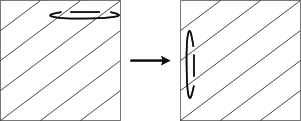
Figure 6: Isotopy in the proof of Corollary 3

Example 2

For $k=2$, Corollary 3 implies that a non-trivial (i.e. $2\leq r_{1}<r_{2}$ and $1\leq s_{1},\ 2\leq s_{2}$) twisted torus link is in fact a torus link if $r_{1}=s_{2}$ and $s_{1}=n\cdot r_{1}$. For example, the Lorenz braid given by $\vec{d}_{L}=\langle 3^{6},8^{3}\rangle$ represents a torus knot:

$$T((3,6),(8,3))=T((3,6),(3,8))=T(3,14)$$

In addition, because the Lorenz braids given by $\vec{d}_{L}=\langle 3^{6},8^{3}\rangle$ and $\langle 3^{14}\rangle$ represent the same link, we see that the integer $k$ is not an invariant of link type.

Going in the opposite direction, a natural symmetry of Lorenz links provides a far-reaching application of Theorem 1 to T-links. Observe that a rotation of $\pi$ about the $z$ axis in Figure 1 is a symmetry of the Lorenz template. If a Lorenz braid $\overline{\mathbb{L}}$ is obtained from a Lorenz braid $\mathbb{L}$ by this rotation, we will say that $\mathbb{L}$ and $\overline{\mathbb{L}}$ are dual Lorenz braids. Both $\mathbb{L}$ and $\overline{\mathbb{L}}$ determine the same Lorenz link $\mathcal{L}$. By Theorem 1, there is a corresponding duality between T–braid representations of $\mathcal{L}$, which vastly generalizes the well-known duality for torus links, T$(r,s)=$T$(s,r)$.

Corollary 4

Let

$$\overline{r}_{1}=s_{k},\ \ \overline{r}_{2}=s_{k}+s_{k-1},\ \ \dots,\ \ \overline{r}_{k}=s_{k}+s_{k-1}+\cdots+s_{1}$$ (14)

$$\overline{s}_{1}=r_{k}-r_{k-1},\ \ \overline{s}_{2}=r_{k-1}-r_{k-2},\ \ \dots,\ \ \overline{s}_{k-1}=r_{2}-r_{1},\ \ \overline{s}_{k}=r_{1}.$$ (15)

Then T$((r_{1},s_{1}),\ldots,(r_{k},s_{k}))$  and  T$((\overline{r}_{1},\overline{s}_{1}),\ldots,(\overline{r}_{k},\overline{s}_{k}))$ have the same link type.

Proof:  By Theorem 1, the claim can be proved for a pair of dual Lorenz braids. Let $\mathcal{L}$ be a Lorenz link with a Lorenz braid representation $\mathbb{L}$, defined by

$$\vec{d}_{L}=\langle d_{1},d_{2},\dots,d_{p}\rangle=\langle r_{1}^{s_{1}},r_{2}^{s_{2}},\dots,r_{k}^{s_{k}}\rangle$$

We claim that $\mathcal{L}$ also has a dual Lorenz braid representation $\overline{\mathbb{L}}$, defined by the dual vector

$$\overline{\vec{d}_{L}}=\langle\overline{d}_{1},\overline{d}_{2},\dots,\overline{d}_{\overline{p}}\rangle=\langle\overline{r}_{1}^{\overline{s}_{1}},\overline{r}_{2}^{\overline{s}_{2}},\dots,\overline{r}_{k}^{\overline{s}_{k}}\rangle$$

with $\overline{p}=d_{p}$ and $\overline{d}_{\overline{p}}=p$, and the rest of the entries determined by $\vec{d}_{L}$ as in (14) and (15). This would imply that $\mathbb{L}$ and $\overline{\mathbb{L}}$ have the same braid index, $p+d_{p}=\overline{p}+\overline{d}_{\overline{p}}$, and both represent $\mathcal{L}$. This correspondence is equivalent to the statement in the theorem: for every T–braid representation of $\mathcal{L}$ in $B_{r_{k}}$, there is a dual T–braid representation of $\mathcal{L}$ in $B_{p}$, given by (14) and (15).

The strands in $\mathbb{L}$ divide into overcrossing strands and undercrossing strands, whose roles are interchanged when we pass from $\mathbb{L}$ to $\overline{\mathbb{L}}$. See Figure 3. From this it follows that $\overline{p}=d_{p}$ and $\overline{d}_{\overline{p}}=p.$ But then $p+d_{p}=\overline{p}+\overline{d}_{\overline{p}}$, so that both have the same braid index. The dual braid is then simply the original one, flipped over so that strand $i$ becomes strand $p+d_{p}-i+1$. Clearly both determine the same link $\mathcal{L}$.

A crossing point in the braid $\mathbb{L}$ or $\overline{\mathbb{L}}$ means a double point in the projected image. Two overcrossing strands in $\mathbb{L}$, (and also in $\overline{\mathbb{L}}$) are said to be parallel when they contain the same number of crossing points. Observe that the overcrossing strands in $\mathbb{L}$ divide naturally into packets of parallel strands, where the $i^{\rm th}$ group of parallel strands contains $s_{i}$ strands, each of which has $r_{i}$ crossing points. In the same way, there is a different subdivision of the overcrossing strands of $\overline{\mathbb{L}}$, with the $j^{\rm th}$ group of parallel strands containing $\overline{s}_{j}$ strands, each having $\overline{r}_{j}$ crossings.

Now observe that there are blank spaces between the endpoints of the $i^{\rm th}$ and $(i+1)^{\rm st}$ group of overcrossing strands in $\mathbb{L}$ for exactly $r_{i+1}-r_{i}$ overcrossing strands of $\overline{\mathbb{L}}$. Taking into account that strand $i$ in $\mathbb{L}$ becomes strand $n-i+1$ in $\overline{\mathbb{L}}$, it follows that $\overline{s}_{k}=r_{1}$ and $\overline{s}_{i}=r_{k-i+1}-r_{k-i}$ if $i>1$. This is the formula (15). Finally, observe that the $j^{\rm th}$ group of overcrossing strands in $\overline{\mathbb{L}}$, where $j=1,2,\dots,k$ intersects precisely $s_{k}+\cdots+s_{k-(j-1)}$ overcrossing strands of $\mathbb{L}$. This gives the formula (14). $\blacksquare$

Example 3

We give some examples of dual Lorenz vectors.

1. $k=1$:  $\langle r^{s}\rangle$ and $\langle s^{r}\rangle$ are dual vectors, so T$(r,s)=$T$(s,r)$.

2. $k=2$:  $\langle r_{1}^{s_{1}},\ r_{2}^{s_{2}}\rangle$  and  $\langle s_{2}^{r_{2}-r_{1}},\ (s_{1}+s_{2})^{r_{1}}\rangle$  are dual,
               so T$((r_{1},s_{1}),(r_{2},s_{2}))\ =\ {\rm T}((s_{2},r_{2}-r_{1}),(s_{1}+s_{2},r_{1}))$.

3. The example in Figure 3: $\langle 2^{4},3^{2},6,8^{2}\rangle$ and $\langle 2^{2},3^{3},5,9^{2}\rangle$ are dual.

4. $\langle 2^{2},\ 3^{3},\ 4^{2},\ 7,\ 9,\ 13^{2}\rangle$  and  $\langle 2^{4},\ 3^{2},\ 4^{3},\ 6,\ 9,\ 11^{2}\rangle$ are dual.

Remark 1

By defintion, Lorenz braids are positive. However, T–links arise naturally as a subset of generalized twisted torus links, which need not be positive. These are defined as in (1), except we now allow $s_{i}\in\mathbb{Z}$; if $s_{i}<0$, the braid generators in that syllable are negative.

Many of our results for T–links were obtained using the duality of the Lorenz template. Without positivity, there is no obvious duality, but some of our results for T–links may still hold for generalized twisted torus links.

General twisted torus links are given by T$((r,s),(p,q))$ with $p>r>0$. If our duality holds, then $T((r,s),(p,q))=T((q,p-r),(q+s,r))$, which implies that $q+s>q>0$, hence $q,s>0$. Therefore, duality as in Corollary 4 applies only to positive twisted torus links.

Question 2

Does another kind of duality apply to non-positive twisted torus links?

3.2 Upper bound for hyperbolic volume

Having the duality formulas of Corollary 4 on hand, we are ready to establish that the volume of hyperbolic Lorenz knots is bounded by a constant that depends only on the size of the Lorenz vector. If $\mathcal{L}$ is obtained by Dehn surgery on a link $Y$, then by Thurston’s Dehn surgery theorem [25], the hyperbolic volume of $\mathcal{L}$ is less than the hyperbolic volume of $Y$. This theorem has many other implications that are easier to explore using T–links. For example, it follows that for any $1\leq i\leq k$, there is a link $Y$ with an unknotted component whose volume is given by

$$\lim_{n\to\infty}{\rm Vol}({\rm T}((r_{1},s_{1}),\ldots,(r_{i-1},s_{i-1}),(r_{i},n\cdot r_{i}),(r_{i+1},s_{i+1}),\ldots,(r_{k},s_{k}))).$$

Thurston’s Dehn surgery theorem together with our results shows that the volume is bounded for many infinite collections of Lorenz links:

Corollary 5

Let $N>0$. Let $\mathcal{L}$ be a hyperbolic Lorenz link such that its Lorenz vector has either $p\leq N$ or $d_{p}\leq N$; equivalently, its T–braid has either $r_{k}\leq N$ or $(s_{1}+\ldots+s_{k})\leq N$. Then the hyperbolic volume of $\mathcal{L}$ is bounded by a constant that depends only on $N$.

Proof:  By Theorem 1, we can establish the claim for T–links for which $r_{k}\leq N$ or $(s_{1}+\ldots+s_{k})\leq N$. Because of the special form for T–braids in (1), we can express the twists of $\mathcal{L}$ as Dehn surgeries on a nested sequence of unknots, $\{(U_{i},n_{i})\}$, as in the proof of Corollary 3. Namely, for each $1\leq i\leq k$, we can find some integers $n_{i}\geq 0,\ 0<a_{i}\leq r_{i}$ such that $s_{i}=n_{i}\cdot r_{i}+a_{i}$. Then, for all $1\leq i\leq k$, we perform a $1/n_{i}$–Dehn surgery on $U_{i}$, augmented to T$((r_{1},s_{1}),\ldots,(r_{i-1},s_{i-1}),(r_{i},a_{i}),(r_{i+1},s_{i+1}),\ldots,(r_{k},s_{k}))$.

Therefore, if $r_{k}\leq N$, $\mathcal{L}$ is obtained by some Dehn surgeries on a fixed finite collection of links. For $\mathcal{L}$ such that $s_{1}+\ldots+s_{k}\leq N$, by Corollary 4, we consider the dual T–link, with $\overline{r}_{k}\leq N$. So every $\mathcal{L}$ is obtained by Dehn surgeries on a fixed finite collection of links, which are given by closed T–braids augmented with unknots. The claim now follows by Thurston’s Dehn surgery theorem. $\blacksquare$

3.3 Polynomial invariants of Lorenz links

Polynomial invariants for certain infinite families of T–links are known. As another application of Theorem 1, we obtain the first such invariants for infinite families of Lorenz links. For the Jones polynomial, twisting formulas were given in Theorem 3.1 of [6]. Thus, the Jones polynomial of an infinite family of links can be obtained from that of any one sufficiently twisted base case.

The Jones polynomials of Lorenz links are highly atypical. The polynomials are often sparse, nonzero coefficients are very small, and the $L^{1}$-norm of coefficients is several orders of magnitude less than for typical links with the same crossing number. Mahler measure is a natural measure on the space of polynomials for which these kinds of polynomials are simplest. Accordingly, the Mahler measure of Jones polynomials of Lorenz links is unusually small, even when their span, which is a lower bound for crossing number, is large.

In [6], it was shown that the Mahler measure of the Jones polynomial converges under twisting for any link: Let $M(V_{\mathcal{L}})$ denote the Mahler measure of the Jones polynomial $V_{\mathcal{L}}$ of $\mathcal{L}$. For any $1\leq i\leq k$, there is a 2-variable polynomial $P$ such that

$$\lim_{n\to\infty}M(V_{{\rm T}((r_{1},s_{1}),\ldots,(r_{i-1},s_{i-1}),(r_{i},n\cdot r_{i}),(r_{i+1},s_{i+1}),\ldots,(r_{k},s_{k}))})=M(P)$$

Thus, the atypical Jones polynomials of Lorenz links may be better understood from the point of view of T–links. For example, the following result is similar to Corollary 5:

Corollary 6

Let $N>0$. Let $\mathcal{L}$ be a Lorenz link such that its Lorenz vector has either $p\leq N$ or $d_{p}\leq N$; equivalently, its T–braid has either $r_{k}\leq N$ or $s_{1}+\ldots+s_{k}\leq N$. Then the Mahler measure of the Jones polynomial of $\mathcal{L}$ is bounded by a constant that depends only on $N$.

Proof:  The proof follows that of Corollary 5, except that at the end, the Dehn surgery theorem is replaced by the $L^{2}$–bound for Mahler measure, as we explain below.

Let $L={\rm T}((r_{1},a_{1}),\ldots,(r_{k},a_{k}))$, as in the proof of Corollary 5. For ${\mathbf{n}}=(n_{1},\ldots,n_{k})$, construct $L_{\mathbf{n}}$ by $1/n_{i}$–Dehn surgeries on $U_{i}$, for $1\leq i\leq k$. By the proof of Corollary 2.3 of [6], there is a $(k+1)$–variable polynomial $P(t,x_{1},\ldots,x_{k})$ that depends only on $L$, such that $M(V_{L_{\mathbf{n}}}(t))=M\left(P(t,t^{n_{1}},\ldots,t^{n_{k}})\right)$.

If $||P||$ denotes the $L^{2}$–norm of coefficients of $P$, then $M(P)\leq||P||$. Therefore,

$$M(V_{L_{\mathbf{n}}}(t))=M\left(P(t,t^{n_{1}},\ldots,t^{n_{k}})\right)\leq||P(t,t^{n_{1}},\ldots,t^{n_{k}})||\leq||P(t,x_{1},\ldots,x_{k})||$$

So if $r_{k}\leq N$, $M(V_{\mathcal{L}})$ is bounded by $\max_{j}(||P_{j}||)$, for a fixed finite collection of polynomials $P_{j}$. $\blacksquare$

Pierre Dehornoy has found many examples of distinct Lorenz knots with the same Jones polynomial, with some pairs that have the same Alexander polynomial as well [11]. For example,

$$\langle 4,4,5,7,7,7,7,7\rangle\quad\text{and}\quad\langle 2,3,4,5,5,6,6,6,6,6\rangle$$

have a common Jones polynomial but different hyperbolic volume. The first knot above is also the knot $K7_{75}$ in the census of simplest hyperbolic knots (see Section 5). The Jones polynomials of these and most other geometrically simple knots were computed in [7].

No general formula is known for Jones polynomials of Lorenz links, even though calculations suggest that their Jones polynomials are very special. We now give a statement that is true for all links that are closed positive braids, and so in particular for all Lorenz links. Our focus has been on the Jones polynomial, but it seems appropriate to also mention related results for the Homflypt and Alexander polynomials P_L and $\Delta_{\mathcal{L}}$:

Corollary 7

[8, 13, 19, 24]. Let $\mathcal{L}$ be a link which is represented as a closed positive $n$–braid $L$. Let $c,\,\mu,\,u,\,g,$ be the number of crossings of $L$, the number of components, the unknotting number and the genus of $\mathcal{L}$. Then the following hold:

$$2\min\deg({\rm V}_{\mathcal{L}}) = 2g+\mu-1=2u-\mu+1=c-n+1$$

$$= \max\deg(\Delta_{\mathcal{L}})=\max\deg_{z}({\rm P}_{\mathcal{L}})=\min\deg_{v}({\rm P}_{\mathcal{L}})$$

The Jones polynomials of twisted torus links T$((r_{1},s_{1}),(r_{2},s_{2}))$ are prime candidates for experiments because they are determined by four integer parameters, i.e. $r_{1},s_{1},r_{2},s_{2}$. If we peek ahead to Corollary 8 we will see that the minimum braid index is a known function of these parameters. Moreover, we know that any invariant, including the Jones polynomial, must satisfy the duality of the defining parameters.

Question 3

What is the Jones polynomial of T$((r_{1},s_{1}),(r_{2},s_{2}))$?

We turn briefly to the Alexander polynomial. By Theorem 1, we can find the Alexander polynomial for a non-trivial infinite family of Lorenz links that are not torus links. We use the fact that Morton [21] computed the Alexander polynomial of T$((2,2m),(p,q))$,

$$\Delta_{\rm T}=\frac{1-t}{(t^{p}-1)(t^{q}-1)}\left(1-(1-t)(1+t^{2}+\ldots+t^{2m-2})(t^{a}+t^{b})-t^{pq+2m}\right)$$

Here, $a=pv$ and $b=(p-u)q$ where $0<u<p,\ 0<v<q$ and $uq\equiv-1\mod p$, $pv\equiv 1\mod q$. By Theorem 1 this is the Alexander polynomial of the Lorenz link with defining vector $\langle 2^{2m},p^{q}\rangle$.

3.4 Braid index formulae

By [14], the braid index $t$ of a Lorenz link is easily computed, one example at a time, from the definition of the trip number $t$ that we gave in (4), but it is unclear how $t$ is related to the parameters $\{(r_{i},s_{i}),\ i=1,\dots,k\}$. Our next application gives a formula for the braid index which depends in a simple way on the defining parameters.

Corollary 8

Let $\mathcal{L}$ be the T–link T$((r_{1},s_{1}),\ldots,(r_{k},s_{k}))$. Let $r_{0}=\overline{r}_{0}=0$, so we can define using (14),

$$i_{0}=\min\{\ i\ |\ r_{i}\geq\overline{r}_{k-i}\}\quad{\rm and}\quad j_{0}=\min\{\ j\ |\ \overline{r}_{j}\geq r_{k-j}\}$$

Then the braid index of $\mathcal{L}$ is $t(\mathcal{L})=\min(r_{i_{0}},\,\overline{r}_{j_{0}})$.

If $k=2$, the braid index of any positive twisted torus link T$((r_{1},s_{1}),(r_{2},s_{2}))$ is given by:

$$t=\begin{cases}\min(s_{2},\ r_{2})&{\rm if}\ r_{1}\leq s_{2}\\ \min(s_{1}+s_{2},\ r_{1})&{\rm if}\ r_{1}\geq s_{2}\end{cases}$$

If $k=1$, i.e. torus links, our formula reduces to the well known fact that the braid index of T$(r,s)$ is $\min(r,s)$.

Proof:  As a Lorenz link, $\mathcal{L}$ is defined by $\vec{d}_{L}=\langle r_{1}^{s_{1}},\ldots,r_{k}^{s_{k}}\rangle$. Below, we use the notation in (2) and (3) with $r_{\mu_{i}}=d_{i}$, so that the following are equivalent:

$$i+d_{i} \geq p$$

$$s_{1}+\ldots+s_{\mu_{i}}+r_{\mu_{i}} \geq s_{1}+\ldots+s_{k}$$

$$r_{\mu_{i}} \geq s_{\mu_{i}+1}+\ldots+s_{k}$$

$$r_{\mu_{i}} \geq \overline{r}_{k-\mu_{i}}$$

Therefore, $\displaystyle i_{0}=\min\{\ \mu_{i}\ |\ i+d_{i}\geq p\}$ and $\displaystyle j_{0}=\min\{\ \mu_{j}\ |\ j+\overline{d}_{j}\geq\overline{p}=d_{p}\}$.

Since displacements correspond to intersecting strands, the $i$-th overcrossing strand crosses $d_{i}$ undercrossing strands. Thus, by (4), $t$ is the number of LR-strands, which equals the number of RL-strands. We now consider two cases.

Case 1. There exists $i_{*}$ such that $i_{*}+d_{i_{*}}=p$.

The left strand $\alpha$ starting at $i_{*}$ with endpoint $p$ is the last LL-strand, so it does not intersect any RR-strands. The equality implies that all RL strands intersect $\alpha$, so $d_{i_{*}}=|$RL$|$. For all $i<i_{*}$, $i+d_{i}<p$, so $i_{0}\geq\mu_{i_{*}}$. For all $i\geq i_{*}$, $r_{\mu_{i}}\geq|$RL$|=r_{\mu_{i_{*}}}$, so $i_{0}=\mu_{i_{*}}$. Therefore,

$$t=|{\rm RL}|=d_{i_{*}}=r_{i_{0}}$$

Case 2. There does not exist $i_{*}$ such that $i_{*}+d_{i_{*}}=p$.

There exists a right strand $\gamma$ with endpoint $p$, which is the first RL-strand. Because its endpoint is $p$, $\gamma$ intersects all LR-strands and no LL strands. In the dual Lorenz link $\overline{\mathcal{L}}$, if $\gamma$ starts at $j_{*}$ then $\overline{d}_{j_{*}}=|$LR$|$. By duality, the endpoint of $\gamma$ is $\overline{p}+1$. If another strand $\gamma^{\prime}$ is parallel to $\gamma$ with endpoint $\overline{p}$ then both strands are in the same packet, so $t=\overline{d}_{j_{*}}=\overline{r}_{j_{0}}$ by Case 1 applied to $\overline{\mathcal{L}}$. Otherwise, for all $j<j_{*}$, $\overline{d}_{j}<\overline{d}_{j_{*}}$ so $j+\overline{d}_{j}<\overline{p}$, hence $j_{0}\geq\mu_{j_{*}}$. For all $j\geq j_{*}$, $\overline{r_{j}}\geq|LR|=\overline{r}_{\mu_{j_{*}}}$, so $j_{0}=\mu_{j_{*}}$. Therefore,

$$t=|{\rm LR}|=\overline{d}_{j_{*}}=\overline{r}_{j_{0}}$$

In both cases, $r_{i_{0}},\overline{r}_{j_{0}}\geq t$, so $t=\min(r_{i_{0}},\overline{r}_{j_{0}})$.

Now let’s specialize to the case $k=2$. If $r_{1}\geq s_{2}=\overline{r}_{1}$ then either case below occurs:

1. $r_{1}\geq\overline{r}_{2}>\overline{r}_{1}\quad\Rightarrow\quad t=\overline{r}_{2}=s_{1}+s_{2}$

2. $\overline{r}_{2}\geq r_{1}\geq\overline{r}_{1}\quad\Rightarrow\quad t=r_{1}$

If $\overline{r}_{1}=s_{2}\geq r_{1}$ then either case below occurs:

1. $r_{2}\geq\overline{r}_{1}\geq r_{1}\quad\Rightarrow\quad t=\overline{r}_{1}=s_{2}$

2. $\overline{r}_{1}\geq r_{2}>r_{1}\quad\Rightarrow\quad t=r_{2}$

When $k=1$, the Lorenz braid defined by $d_{L}=\langle r^{s}\rangle$ represents the torus link T$(r,s)$, which is the closure of the $r$-braid $(\sigma_{1}\dots\sigma_{r-1})^{s}$. The dual Lorenz braid $\langle s^{r}\rangle$ represents the same torus link T$(s,r)$, which is the closure of the $s$-braid $(\sigma_{1}\dots\sigma_{s-1})^{r}$. As is well known, the braid index of a torus link is $\min(r,s)$, which agrees with Corollary 8. $\blacksquare$

4 Minimal braid index representations

We have proved that there are different closed braid representations of a Lorenz link $\mathcal{L}$, with braid indices: $p+d_{p},\ d_{p},\ p$, and $t$. The representation of braid index $p+d_{p}$ is the Lorenz braid defined by our vector $d_{L}=\langle r_{1}^{s_{1}},\dots,r_{k}^{s_{k}}\rangle$. The representation of braid index $d_{p}=r_{k}$ was given in Theorem 1, and its dual $p$–braid in Corollary 4. In this section, we use Lemma 1 and some of the things we have learned along the way, to establish another correspondence, this time between Lorenz braid representations of $\mathcal{L}$ (hence also T–braid representations) and special $t$–braid representations, where $t$ is the minimal braid index of $\mathcal{L}$.

Let $\mathbb{L}$ be a Lorenz braid defined by $\vec{d}_{L}=\langle d_{1},d_{2},\dots,d_{p}\rangle$, representing the Lorenz link $\mathcal{L}$. As discussed earlier, the strands in $\mathbb{L}$ divide into strands of type LL, LR,RL and RR, where strand $j$ has type LL if and only if $1\leq j\leq p-t$. By duality, strand $j$ has type RR if and only if strand $\overline{j}$ has type LL with respect to $\overline{\mathbb{L}}$; i.e., $1\leq\overline{j}\leq\overline{p}-t=d_{p}-t$. We define

$$n_{i} = \#\{{\rm strand}\ j\in{\rm LL\quad such\ that}\quad d_{j}=i+1\},$$ (16)

$$m_{i} = \#\{{\rm strand}\ j\in{\rm RR\quad such\ that}\quad\overline{d}_{\overline{j}}=i+1\}.$$ (17)

Let $\vec{n}=(n_{1},\dots,n_{t-1})$, $\vec{m}=(m_{1},\dots,m_{t-1})$, where each $n_{i},\;m_{j}\geq 0$. The conditions in (3) are automatically satisfied for any $\vec{n},\ \vec{m}$ with non-zero entries. In Example 1, for which $t=3$, we get $n_{1}=4,\ n_{2}=2,\ m_{1}=2,\ m_{2}=3$, which is immediate from Figure 3.

The triple $(t,\vec{n},\vec{m})$, $t\geq 2$, defines the following $t$–braid representation of $\mathcal{L}$, where $t$ is the braid index of $\mathcal{L}$:

$$\mathbb{M} = (\sigma_{1}\cdots\sigma_{t-1})^{t}\ \ \prod_{i=1}^{t-1}\,(\sigma_{1}\cdots\sigma_{i})^{n_{i}}\ \prod_{i=t-1}^{1}\,(\sigma_{t-1}\cdots\sigma_{i})^{m_{t-i}}$$ (18)

$$= [1,t]^{t}\ \ \prod_{i=1}^{t-1}\,[1,i+1]^{n_{i}}\ \prod_{i=t-1}^{1}\,[t,i]^{m_{t-i}}$$

$$= [1,t]^{t}\ \ \prod_{i=1}^{t-1}\,[1,i+1]^{n_{i}}\ \ \prod_{i=1}^{t-1}\ [t,t-i]^{m_{i}}$$

This was proved in Proposition 5.6 of [3], with a small but very confusing typo corrected. The proof of Proposition 5.6 of [3] is correct, but the formula there is not. The following theorem is a strengthening of Proposition 5.6 of [3], and is comparable to Theorem 1: It sets up a correspondence between Lorenz braid representations of $\mathcal{L}$ and special $t$–braid representations.

Theorem 2

There is a one-to-one correspondence between Lorenz braids $\mathbb{L}\in B_{p+d_{p}}$, with defining vector $\vec{d}_{L}$ as in (2), and triples $(t,\vec{n},\vec{m})$, which determine a $t$-braid $\mathbb{M}$.

Caution: Distinct Lorenz braid representations of $\mathcal{L}$, and their corresponding distinct triples $(t,\vec{n},\vec{m})$, may determine the same $t$-braid representation $\mathbb{M}$ of $\mathcal{L}$. For example, when $t=2$ the only possibility is $\vec{n}=(n_{1}),\ \ \vec{m}=(m_{1})$, where $n_{1}$ and $m_{1}$ are both positive, so that $\mathbb{M}=\sigma_{1}^{2+n_{1}+m_{1}}$. Other partitions of $n_{1}+m_{1}$ will give other triples $(t,\vec{n},\vec{m})$ but the same 2-braid.

Proof:  The reader is referred to [3] for the proof that $\mathbb{L}$ determines $\mathbb{M}$. We will prove the converse.

We first prove that $(t,\vec{n},\vec{m})$ determines the subvector $\vec{d}_{LL}\subset\vec{d}_{L}$ consisting of all $d_{i}$ such that $i\leq|$LL$|$. In the proof of Lemma 1, we uncoiled the LL–braid to construct the equivalent $t$–strand braid $\mathbb{X}$, given in (7). Namely, we traded each braid strand in LL, together with its associated loop around the axis, for an arc corresponding to one of the sequences $(\sigma_{1}\sigma_{2}\cdots\sigma_{d_{j}-1})$ in the braid word $\mathbb{X}$. The definition of $n_{i}$ implies that

$$\mathbb{X}=\prod_{j=1}^{p-t}(\sigma_{1}\sigma_{2}\cdots\sigma_{d_{j}-1})=\prod_{i=1}^{t-1}(\sigma_{1}\sigma_{2}\cdots\sigma_{i})^{n_{i}}$$

This is a subword of $\mathbb{M}$. Going the other way, each subword $(\sigma_{1}\sigma_{2}\cdots\sigma_{i})^{n_{i}}\in\mathbb{M}$ must have come from a group of $n_{i}$ parallel strands in LL. Since the LL braid is made up entirely from groups of parallel strands, it follows that $|$LL$|=n_{1}+\cdots+n_{t-1}$.

Using the now-familar trick of passing from $\mathbb{L}$ to $\overline{\mathbb{L}}$, it follows that $|$RR$|=m_{1}+\cdots+m_{t-1}$. Note also that, since $p=|$LL$|+t$ and $d_{p}=|$RR$|+t$, it follows that the braid index of $\mathbb{L}$ is

$$p+d_{p}=2t+\sum_{i=1}^{t-1}(n_{i}+m_{i}).$$

Therefore, $(t,\vec{n},\vec{m})$ determines (i) the braid index of $\mathbb{L}$, (ii) the number $|$LL$|$ of strands in the LL braid and (iii) the subvector $\vec{d}_{LL}\subset\vec{d}_{L}$. By duality, $(t,\vec{m},\vec{n})$ then also determines $\vec{d}_{RR}$. Next, notice that the only strands of $\mathbb{L}$ which have endpoints in R are type RR and LR, and from this it follows that all endpoint positions in R which are not occupied by strands of type RR must be occupied by the strands of type LR. Moreover, the endpoints of the LR strands are completely determined because there are no crossings between pairs of strands of type LR. Since we already know the vector $\vec{d}_{LL}$, it follows that the vector $\vec{d}_{L}$ is completely determined. Likewise, $\vec{d}_{R}$ is determined, hence $\mathbb{L}$ is completely determined by $(t,\vec{n},\vec{m})$. $\blacksquare$

Remark 2

Using Theorem 2, we get a second proof of Corollary 2. By Corollary 1 $(ii)$, for fixed braid index, the letter length of any braid representation is a topological invariant of $\mathcal{L}$. Let $t$ be the trip number of $\mathcal{L}$. Since only finitely many positive words have given letter length, there are finitely many $t$–braid representations of $\mathcal{L}$ of the form (18). By Theorem 2, $\mathcal{L}$ has finitely many Lorenz braid representations of the form (2); i.e., up to trivial stabilizations.

Remark 3

Corollary 4 results in a duality for $t$–braids, given by conjugation by the half-twist $\Delta$, which sends every $\sigma_{i}$ to $\sigma_{t-i}$. For every $t$–braid as in (18), we get another braid in the same conjugacy class and which has the special form given in (18). To see this, note that conjugation by $\Delta$ sends

$$\mathbb{M}=[1,t]^{t}\prod_{i=1}^{t-1}[1,i+1]^{n_{i}}\prod_{i=1}^{t-1}[t,t-i]^{m_{i}}$$

to

$$\Delta\mathbb{M}\Delta^{-1}=[t,1]^{t}\prod_{i=1}^{t-1}[t,t-i]^{n_{i}}\prod_{i=1}^{t-1}[1,i+1]^{m_{i}}\approx[1,t]^{t}\prod_{i=1}^{t-1}[1,i+1]^{m_{i}}\prod_{i=1}^{t-1}[t,t-i]^{n_{i}}$$

where $\approx$ means after cyclic permutation. We use the fact that $\Delta^{2}=[1,t]^{t}=[t,1]^{t}$ is in the center of $B_{t}$.

Our experimental data suggests that this is a general phenomenon:

Conjecture 1

If a Lorenz link $\mathcal{L}$ has representations $\mathbb{M}_{1},\ \mathbb{M}_{2}\in B_{t},$ where $t$ is the trip number of $\mathcal{L}$, then $\mathbb{M}_{1},\mathbb{M}_{2}$ are in the same conjugacy class in $B_{t}$.

With regard to this conjecture, Corollary 3 provides many examples of interesting conjugacy between the $t$–braid representations of $\mathbb{L}_{1}$ and $\mathbb{L}_{2}$. In general, links that are closed positive braids need not have unique conjugacy classes of minimum braid representations, but the known examples that might contradict Conjecture 1 cannot be Lorenz links. For example, composite links have minimum closed braid representations that admit exchange moves, leading to infinitely many conjugacy classes of minimum braid index representations, but Lorenz links are prime [28]. Also, links that are closed 3-braids and admit positive flypes have non-unique conjugacy classes, but the Lorenz links of trip number 3 have been studied [1], and they do not include any closed positive 3-braids that admit positive flypes.

There are very few families of links for which we know, precisely, minimum braid index representatives, the most obvious being the unknot itself. In [3] Lorenz braids whose closures define the unknot were delineated precisely. The question of which Lorenz braids determine torus links is more complicated, but is a natural next step. A pair of positive integers $p,q$ suffice to determine the type of any torus link, but looking at the class of all Lorenz links, it is difficult to determine which ones are torus links. With the help of Theorem 2, we are able to make a contribution to that problem:

Corollary 9

Let $\mathcal{L}$ be a Lorenz link with trip number $t$. Let $\mathbb{M}$ be a $t$-braid representative of $\mathcal{L}$, as given in (18). Then there is an algorithm of complexity $O(|\mathbb{M}|^{2}t^{3}\log t)$ that determines whether or not $\mathcal{L}$ is a torus link.

Proof:  By [14], $t$ is the braid index of $\mathcal{L}$. By a theorem of Schubert [23], we know that if $\mathcal{L}$ is a torus link, then it has a minimum braid index representative in $B_{t}$ of the form $[1,t]^{q}$ for some $q\geq t$. Also, by a different result in [23], any closed $t$-braid that represents $\mathcal{L}$ must be conjugate to $[1,t]^{q}$. Our first question is: if $\mathcal{L}$ is a torus link, what is the integer $q$? Since $\mathbb{M}$ and $[1,t]^{q}$ are both positive braids, they must have the same letter length. From this it follows that $\mathcal{L}$ cannot be a torus link unless $|\mathbb{M}|=(t-1)(q)$ . Therefore $q=|\mathbb{M}|/(t-1)$.

We now give an algorithm to decide whether the $t$-braids $\mathbb{L}_{t}$ and $[1,t]^{q}$ are conjugate in $B_{t}$. Changing our viewpoint, we now regard the braid group $B_{t}$ as the mapping class group of the unit disc $D^{2}$ minus $t$ points, where admissible maps fix $\partial D^{2}$. See [2], for example, for a proof that this mapping class group is isomorphic to Artin’s braid group $B_{t}$. Let $\delta$ be the $t$-braid $[1,t]$. If the points which are deleted from the unit disc $D^{2}$ are arranged symmetrically around the circle of radius 1/2, then $\delta$ may be seen as a rotation of angle $2\pi/t$ about the origin, with the boundary of $D^{2}$ held fixed. Such a braid has the Thurston-Nielson type of a periodic braid of period $t$. By the results in [15] we know that periodic braids have unique roots. Therefore it suffices to prove that $(\mathbb{M})^{t}$ is conjugate to $\delta^{qt}$. Observe that $\delta^{t}$ generates the center of $B_{t}$, so that $\delta^{tq}$ is in the center, and from this it follows that it suffices to prove that $\mathbb{M}^{t}$ and $\delta^{tq}$ represent the same element of $B_{t}$. This trick reduces the conjugacy problem to the word problem.

There is a solution to the word problem in $B_{t}$ that was discovered simultaneously by El-Rifai–Morton and by Thurston which has the property: if $X$ is an element of $B_{t}$ which has letter length $|X|$ then its left-greedy normal form can be computed in time $O(|X|^{2}t\log t)$. In our case the word length of $\mathbb{M}^{t}$ is $(t)(|\mathbb{M}|)$, therefore the problem can be solved in time $O(|\mathbb{M}|^{2}t^{3}\log t)$, as claimed. $\blacksquare$

Remark 4

El-Rifai [12] classified all ways in which a Lorenz knot can be presented as a satellite of a Lorenz knot. He showed that only parallel cables with possible twists can occur. These results generalize Theorems 6.2 and 6.5 of [3].

Question 4

Is there an efficient algorithm, along the lines of Corollary 9, to recognize when a Lorenz knot is a satellite of a Lorenz knot?

In relation to the above, a very interesting open problem was posed in [12]:

Question 5

Can a Lorenz knot be a satellite of a non-Lorenz knot?

Noting the method of proof in [28] that Lorenz knots are prime, one suspects that the fact that every Lorenz knot embeds on the Lorenz template implies that the answer is ‘no’. This is an interesting question because one would like very much to know how to separate the hyperbolic Lorenz knots and links from those which are not hyperbolic.

In this regard, we note that the Lorenz braids that determine the unknot were completely characterized in [3]. It seems to be much more difficult to decide:

Question 6

Which Lorenz braids close to torus links?

We have partial results on this problem, but have not found a satisfactory general answer.

5 Lorenz data for the simplest hyperbolic knots

In the table below, we list 107 simplest hyperbolic knots (see [4, 7]) that are Lorenz, and five that are possibly Lorenz; the rest are not Lorenz. The symbol $\mathbf{k}n_{m}$ means the $m$th knot in the census of hyperbolic knots whose complement can be constructed from no less than $n$ ideal tetrahedra.

The 107 identified Lorenz braids in the table were proved to be isometric to the corresponding census knots using SnapPea to verify the isometry. Many had already been identified as positive twisted torus knots in [4, 7].

The 89 simplest hyperbolic knots that are not listed in the table are not Lorenz. For many, their Jones polynomials from [7] failed to satisfy Corollary 7. For the others, we used the following method:

Pierre Dehornoy computed all Lorenz braids up to 49 crossings that close to a knot, and Slavik Jablan eliminated duplications from this list, which contains 14,312 distinct non-alternating Lorenz knots up to 49 crossings. If $c$ is the crossing number of the Lorenz braid and $g$ is the genus of the knot, then by (13), we know that $c\leq 4g$. So any Lorenz knot with $g\leq 12$ has a Lorenz braid representation with $c\leq 48$. Therefore, any knot with $g\leq 12$ that is missing from the Dehornoy–Jablan list cannot be Lorenz.

Knots with 16 or fewer crossings are classified, and their invariants are accessible using Knotscape. For these knots, if the minimal and maximal degrees of their Jones polynomials have the same sign, we verified that the smaller absolute value of the two is less than 12. It follows that $g\leq 12$ for any of these knots that satisfy Corollary 7. Jablan provided us with the following Knotscape knots in the Dehornoy–Jablan list, which is, therefore, the complete classification of Lorenz knots up to 16 crossings:

$$3_{1},\,5_{1},\,7_{1},\,9_{1},\,8_{19},\,10_{124},\,11a_{367},\,12n_{242},\,12n_{725},\,13a_{4878},\,14n_{6022},\,14n_{21324}$$

$$14n_{21881},\,15n_{41185},\,15a_{85263},\,16n_{184868},\,16n_{771177},\,16n_{783154},\,16n_{996934}$$

In addition, Jablan verified for us that $\mathbf{k}6_{31}$, $\mathbf{k}7_{81}$, $\mathbf{k}7_{83}$, $\mathbf{k}7_{106}$, $\mathbf{k}7_{113}$, $\mathbf{k}7_{118}$, $\mathbf{k}7_{124}$, and $\mathbf{k}7_{119}$ are not on the Dehornoy–Jablan list. The remaining four simplest hyperbolic knots, indicated by a “?” in the table below, have diagrams with more than 49 crossings, which cannot be handled by this computer program. Except for $\mathbf{k}7_{119}$, the knots listed have Jones polynomials (see [7]) that imply $g\leq 12$ if they satisfy Corollary 7. Although $\mathbf{k}7_{119}$ has a diagram with 33 crossings, $g=15$, so we cannot be certain that it does not have a Lorenz braid with $50\leq c\leq 60$.

The following formulas, which follow from results earlier in this paper, provide additional information that can be obtained using the Lorenz braids in our final table on the next page. Let $\mathcal{L}$ be any Lorenz link given by $\vec{d}_{L}=\langle d_{1},\dots,d_{p}\rangle$, as in (2). Let $S=\sum_{i=1}^{p}d_{i}$, and let $t$ be its trip number. The crossing numbers and braid indices of the Lorenz braid $\mathbb{L}$, the T–braid $\mathbb{T}$, the dual T–braid $\mathbb{T}^{\prime}$, and the minimal braid index $t$–braid ${\mathbb{M}}$ are as follows:

$\mathbb{L}$ $\mathbb{T}$ $\mathbb{T}^{\prime}$ $\mathbb{M}$ crossing number $S$ $S-p$ $S-d_{p}$ $S+t-p-d_{p}$ braid index $p+d_{p}$ $d_{p}$ $p$ $t$

The braid crossing numbers of the braids $\mathbb{M}$ for some Lorenz knots in the census turn out to be surprisingly high. In fact, the crossing number of the minimum index braid in equation (18) is the minimal crossing number of the Lorenz link, by Proposition 7.4 of [22].

On the next page, we give the table of Lorenz knots that are in the census of hyperbolic knots whose complements can be constructed from seven or fewer ideal tetrahedra.

Knot Lorenz vector Knot Lorenz vector Knot Lorenz vector $\mathbf{k}3_{1}$ $\langle\,2^{2},\,3^{4}\,\rangle$ $\mathbf{k}7_{3}$ $\langle\,2^{2},\,5^{16}\,\rangle$ $\mathbf{k}7_{55}$ $\langle\,5^{2},\,7^{9}\,\rangle$ $\mathbf{k}4_{3}$ $\langle\,2^{2},\,3^{8}\,\rangle$ $\mathbf{k}7_{4}$ $\langle\,3^{3},\,5^{17}\,\rangle$ $\mathbf{k}7_{56}$ ? $\mathbf{k}4_{4}$ $\langle\,2^{2},\,4^{7}\,\rangle$ $\mathbf{k}7_{5}$ $\langle\,2^{4},\,3^{16}\,\rangle$ $\mathbf{k}7_{57}$ $\langle\,3^{6},\,4^{13}\,\rangle$ $\mathbf{k}5_{1}$ $\langle\,2^{2},\,5^{6}\,\rangle$ $\mathbf{k}7_{6}$ $\langle\,3^{2},\,7^{16}\,\rangle$ $\mathbf{k}7_{58}$ $\langle\,4^{4},\,7^{10}\,\rangle$ $\mathbf{k}5_{4}$ $\langle\,2^{2},\,5^{8}\,\rangle$ $\mathbf{k}7_{7}$ $\langle\,2^{2},\,7^{18}\,\rangle$ $\mathbf{k}7_{59}$ $\langle\,5^{4},\,9^{7}\,\rangle$ $\mathbf{k}5_{5}$ $\langle\,2^{2},\,3^{11}\,\rangle$ $\mathbf{k}7_{8}$ $\langle\,2^{2},\,6^{7}\,\rangle$ $\mathbf{k}7_{60}$ $\langle\,7^{7},\,8^{5}\,\rangle$ $\mathbf{k}5_{6}$ $\langle\,3^{3},\,5^{6}\,\rangle$ $\mathbf{k}7_{9}$ $\langle\,10^{2},\,11^{4}\,\rangle$ $\mathbf{k}7_{61}$ $\langle\,7^{10},\,3^{2}\,\rangle$ $\mathbf{k}5_{7}$ $\langle\,2^{2},\,5^{7}\,\rangle$ $\mathbf{k}7_{12}$ $\langle\,3^{2},\,8^{7}\,\rangle$ $\mathbf{k}7_{62}$ $\langle\,8^{8},\,10^{3}\,\rangle$ $\mathbf{k}5_{10}$ $\langle\,4^{2},\,5^{4}\,\rangle$ $\mathbf{k}7_{13}$ $\langle\,2^{2},\,7^{12}\,\rangle$ $\mathbf{k}7_{63}$ $\langle\,4^{2},\,6^{11}\,\rangle$ $\mathbf{k}5_{11}$ $\langle\,2^{6},\,3^{4}\,\rangle$ $\mathbf{k}7_{14}$ $\langle\,2^{2},\,8^{11}\,\rangle$ $\mathbf{k}7_{64}$ $\langle\,4^{4},\,5^{17}\,\rangle$ $\mathbf{k}5_{14}$ $\langle\,3^{2},\,4^{7}\,\rangle$ $\mathbf{k}7_{15}$ $\langle\,10^{4},\,11^{4}\,\rangle$ $\mathbf{k}7_{66}$ $\langle\,5^{3},\,6^{11}\,\rangle$ $\mathbf{k}5_{15}$ $\langle\,4^{4},\,7^{3}\,\rangle$ $\mathbf{k}7_{16}$ $\langle\,5^{3},\,8^{11}\,\rangle$ $\mathbf{k}7_{67}$ $\langle\,8^{4},\,9^{10}\,\rangle$ $\mathbf{k}5_{16}$ $\langle\,5^{5},\,7^{3}\,\rangle$ $\mathbf{k}7_{17}$ $\langle\,3^{2},\,8^{13}\,\rangle$ $\mathbf{k}7_{68}$ $\langle\,2^{6},\,3^{10}\,\rangle$ $\mathbf{k}5_{17}$ $\langle\,4^{4},\,5^{7}\,\rangle$ $\mathbf{k}7_{20}$ $\langle\,5^{2},\,6^{5}\,\rangle$ $\mathbf{k}7_{69}$ $\langle\,7^{4},\,8^{9}\,\rangle$ $\mathbf{k}5_{18}$ $\langle\,4^{8},\,5^{3}\,\rangle$ $\mathbf{k}7_{21}$ $\langle\,2^{2},\,7^{9}\,\rangle$ $\mathbf{k}7_{71}$ $\langle\,6^{6},\,7^{10}\,\rangle$ $\mathbf{k}6_{3}$ $\langle\,2^{2},\,5^{11}\,\rangle$ $\mathbf{k}7_{22}$ $\langle\,3^{3},\,5^{16}\,\rangle$ $\mathbf{k}7_{73}$ $\langle\,8^{6},\,9^{8}\,\rangle$ $\mathbf{k}6_{4}$ $\langle\,3^{3},\,5^{12}\,\rangle$ $\mathbf{k}7_{23}$ $\langle\,5^{15},\,7^{2}\,\rangle$ $\mathbf{k}7_{75}$ $\langle\,3^{3},\,5^{8}\,\rangle$ $\mathbf{k}6_{5}$ $\langle\,2^{2},\,3^{14}\,\rangle$ $\mathbf{k}7_{27}$ $\langle\,3^{2},\,4^{15}\,\rangle$ $\mathbf{k}7_{76}$ $\langle\,6^{12},\,7^{4}\,\rangle$ $\mathbf{k}6_{6}$ $\langle\,3^{2},\,7^{9}\,\rangle$ $\mathbf{k}7_{28}$ $\langle\,4^{8},\,5^{6}\,\rangle$ $\mathbf{k}7_{78}$ $\langle\,6^{12},\,7^{5}\,\rangle$ $\mathbf{k}6_{7}$ $\langle\,2^{2},\,7^{11}\,\rangle$ $\mathbf{k}7_{29}$ $\langle\,7^{2},\,9^{11}\,\rangle$ $\mathbf{k}7_{79}$ $\langle\,3^{2},\,9^{13}\,\rangle$ $\mathbf{k}6_{11}$ $\langle\,2^{2},\,5^{9}\,\rangle$ $\mathbf{k}7_{30}$ $\langle\,2^{2},\,4^{19}\,\rangle$ $\mathbf{k}7_{82}$ $\langle\,4^{4},\,5^{13}\,\rangle$ $\mathbf{k}6_{12}$ $\langle\,3^{3},\,5^{11}\,\rangle$ $\mathbf{k}7_{31}$ $\langle\,5^{3},\,9^{13}\,\rangle$ $\mathbf{k}7_{87}$ $\langle\,5^{5},\,7^{4}\,\rangle$ $\mathbf{k}6_{13}$ $\langle\,2^{2},\,5^{12}\,\rangle$ $\mathbf{k}7_{32}$ $\langle\,8^{4},\,11^{5}\,\rangle$ $\mathbf{k}7_{88}$ $\langle\,5^{15},\,7^{3}\,\rangle$ $\mathbf{k}6_{14}$ $\langle\,3^{2},\,4^{11}\,\rangle$ $\mathbf{k}7_{33}$ $\langle\,6^{2},\,7^{10}\,\rangle$ $\mathbf{k}7_{90}$ $\langle\,2^{6},\,3^{8}\,\rangle$ $\mathbf{k}6_{15}$ $\langle\,6^{6},\,7^{4}\,\rangle$ $\mathbf{k}7_{34}$ $\langle\,4^{2},\,5^{9}\,\rangle$ $\mathbf{k}7_{99}$ $\langle\,2^{2},\,3^{2},\,5^{2}\,\rangle$ $\mathbf{k}6_{16}$ $\langle\,7^{7},\,8^{3}\,\rangle$ $\mathbf{k}7_{35}$ $\langle\,7^{7},\,9^{4}\,\rangle$ $\mathbf{k}7_{101}$ ? $\mathbf{k}6_{17}$ $\langle\,2^{2},\,4^{15}\,\rangle$ $\mathbf{k}7_{36}$ $\langle\,6^{6},\,7^{9}\,\rangle$ $\mathbf{k}7_{102}$ $\langle\,2^{4},\,4^{5}\,\rangle$ $\mathbf{k}6_{18}$ $\langle\,6^{6},\,7^{5}\,\rangle$ $\mathbf{k}7_{37}$ $\langle\,2^{2},\,5^{14}\,\rangle$ $\mathbf{k}7_{109}$ ? $\mathbf{k}6_{19}$ $\langle\,2^{6},\,3^{5}\,\rangle$ $\mathbf{k}7_{38}$ $\langle\,2^{2},\,8^{13}\,\rangle$ $\mathbf{k}7_{110}$ $\langle\,2^{2},\,3^{5},\,5^{4}\,\rangle$ $\mathbf{k}6_{21}$ $\langle\,5^{4},\,8^{7}\,\rangle$ $\mathbf{k}7_{39}$ $\langle\,3^{3},\,11^{2}\,\rangle$ $\mathbf{k}7_{111}$ $\langle\,3^{3},\,7^{10}\,\rangle$ $\mathbf{k}6_{25}$ $\langle\,4^{6},\,5^{4}\,\rangle$ $\mathbf{k}7_{42}$ $\langle\,7^{14},\,8^{3}\,\rangle$ $\mathbf{k}7_{112}$ $\langle\,2^{1},\,5^{4},\,8^{6}\,\rangle$ $\mathbf{k}6_{27}$ $\langle\,3^{3},\,4^{11}\,\rangle$ $\mathbf{k}7_{43}$ $\langle\,6^{2},\,7^{16}\,\rangle$ $\mathbf{k}7_{115}$ $\langle\,3^{5},\,4^{7}\,\rangle$ $\mathbf{k}6_{29}$ $\langle\,3^{6},\,7^{2}\,\rangle$ $\mathbf{k}7_{47}$ $\langle\,4^{4},\,6^{7}\,\rangle$ $\mathbf{k}7_{119}$ ? $\mathbf{k}6_{30}$ $\langle\,4^{4},\,5^{12}\,\rangle$ $\mathbf{k}7_{48}$ ? $\mathbf{k}7_{122}$ $\langle\,4^{2},\,5^{3},\,7^{3}\,\rangle$ $\mathbf{k}6_{32}$ $\langle\,4^{4},\,5^{8}\,\rangle$ $\mathbf{k}7_{50}$ $\langle\,6^{4},\,7^{5}\,\rangle$ $\mathbf{k}7_{123}$ $\langle\,6^{12},\,8^{5}\,\rangle$ $\mathbf{k}6_{35}$ $\langle\,6^{6},\,5^{8}\,\rangle$ $\mathbf{k}7_{51}$ $\langle\,5^{2},\,7^{8}\,\rangle$ $\mathbf{k}7_{126}$ $\langle\,4^{8},\,8^{3}\,\rangle$ $\mathbf{k}6_{36}$ $\langle\,5^{10},\,7^{3}\,\rangle$ $\mathbf{k}7_{52}$ $\langle\,5^{2},\,7^{6}\,\rangle$ $\mathbf{k}6_{39}$ $\langle\,4^{4},\,8^{3}\,\rangle$ $\mathbf{k}7_{53}$ $\langle\,4^{4},\,10^{3}\,\rangle$

References

- [1] R. Bedient, Classifying 3-trip Lorenz knots, Topology and its Applications 20 (1985), 89-96.
- [2] J. Birman and T. Brendle, Braids:A Survey, in “Handbook of Knot Theory”, Editors W. Menasco and M. Thistlethwaite, Elsevier (2005), 19-104.
- [3] J. S. Birman and R. F. Williams, Knotted Periodic Orbits in Dynamical Systems-I: Lorenz’s Equations, Topology 22, No. 1 (1983), 47-82.
- [4] P. Callahan, J. Dean, J. Weeks, The simplest hyperbolic knots, J. Knot Theory Ramifications 3 (1999), 279-297.
- [5] P. Callahan, M. Hildebrand, J. Weeks, A census of cusped hyperbolic 3-manifolds, Mathematics of Computation 68, No. 225 (1999), 321-332.
- [6] A. Champanerkar, I. Kofman, On the Mahler measure of Jones polynomials under twisting, Algebr. Geom. Topol. 5 (2005), 1-22.
- [7] A. Champanerkar, I. Kofman, E. Patterson, The next simplest hyperbolic knots, J. Knot Theory Ramifications 13 (2004), 965-987.
- [8] P. R. Cromwell, Homogeneous links, J. London Math Soc. 39, No. 2 (1989), 535-552.
- [9] J. Dean, Hyperbolic knots with small Seifert-fibered Dehn surgeries, Ph.D. thesis, University of Texas at Austin, May 1996.
- [10] Pierre Dehornoy, Noeuds de Lorenz, preprint available at http://www.eleves.ens.fr/home/dehornoy/maths/Lorenz4.pdf.
- [11] Pierre Dehornoy, private communication, June 2008.
- [12] E. El-Rifai, Necessary and sufficient conditions for Lorenz knots to be closed under satellite construction, Chaos, Solitons & Fractals 10 (1999), 137-146.
- [13] T. Fiedler, On the degree of the Jones polynomial, Topology 30 (1991), 1-8.
- [14] J. Franks and R.F.Williams, Braids and the Jones polynomial, Trans. AMS 303, No. 1 (1987), 97-108.
- [15] J. González-Meneses, The root of a braid is unique up to conjugacy. Algebraic and Geometric Topology 3 (2003), 1103-1118.
- [16] E. Ghys, Knots and Dynamics, preprint, to appear in Proc ICM-2006, Madrid.
- [17] E. Ghys, private communication, July 2007.
-
[18]
E. Ghys and J. Leys, Lorenz and Modular Flows: A Visual Introduction, AMS Feature Column, Nov. 2006,
http://www.ams.org/featurecolumn/archive/lorenz.html. - [19] T. Kawamura, Relations among the lowest degree of the Jones polynomial and geometric invariants for closed positive braids, Comment. Math. Helv. 77 (2002), 125-132.
- [20] E. N. Lorenz, Deterministic non-periodic flow, J. Atmospheric Science 20 (1963), 130-141.
- [21] H. Morton, The Alexander polynomial of a torus knot with twists, J. Knot Theory Ramifications 15 (2006), 1037-1047.
- [22] K. Murasugi, On the braid index of alternating links, Trans. Amer. Math. Soc. 326, no. 1, 237-260.
- [23] H Schubert, Knoten und Vollringe, Acta Math. 90 (1953), 131 226.
- [24] A. Stoimenow, Positive knots, closed braids and the Jones polynomial, Ann. Scuola Norm. Sup. Pisa Cl. Sci. 5 2(2) (2003), 237–285, arXiv:math.GT/9805078.
-
[25]
W. Thurston, The Geometry and Topology of Three-Manifolds,
electronic 1.1 (2002), http://www.msri.org/publications/books/gt3m/ - [26] W. Tucker, A rigorous ODE solver and Smale’s 14th problem, Found. Comput. Math. 2 (2002), 53-117.
- [27] M. Viana, What’s new on Lorenz strange attractors, Math. Intelligencer 22, No. 3 (2000), 6-19.
- [28] R. F. Williams, Lorenz knots are prime, Ergodic Theory and Dynamical Systems 4 (1983), 147-163.