Accelerating Cosmologies in the Einstein-Gauss-Bonnet Theory with Dilaton

Abstract

We study cosmological solutions in the low-energy effective heterotic string theory, which is the Einstein gravity with Gauss-Bonnet term and the dilaton. We show that the field equations are cast into an autonomous system for flat internal and external spaces, and derive all the fixed points in the system. We also examine the time evolution of the solutions and whether the solutions can give (transient) accelerated expansion of our four-dimensional space in the Einstein frame.

1 Introduction

The recent cosmological observations have confirmed the existence of the early inflationary epoch and the accelerated expansion of the present universe [1]. An important problem is then to derive such a model from fundamental theories of particle physics. The most promising candidates for such theories are the ten-dimensional superstrings or eleven-dimensional M-theory, which are hoped to give models of accelerated expansion of the universe upon compactification to four dimensions. There are many attempts to derive such models, but most of them assume some additional matters or need special settings. From the viewpoint of the fundamental theories, however, it is desirable if such models are obtained without making special assumptions.

It has been shown that a model with certain period of accelerated expansion can be obtained from the higher-dimensional vacuum Einstein equation if one assumes a time-dependent hyperbolic internal space [2] and that this class of models is obtained [3] from what are known as S-branes [4, 5] in the limit of vanishing flux of three-form fields (see also Ref. Sbrane3). For other attempts at inflation in the context of string theories, see, for instance, Refs. other,chen,Kachru. Unfortunately this class of models do not give sufficient inflation necessary to resolve the cosmological problems.

On the other hand, it has been known that higher order corrections can give rise to inflationary solutions. [10] This is a very desirable setting since there are terms of higher orders in the curvature to the lowest effective supergravity action coming from superstrings or M-theory [11, 12, 13, 14]. The simplest such correction is the Gauss-Bonnet (GB) term in the low-energy effective heterotic string. (We ignore other gauge fields and forms for simplicity.) It is thus important to examine what kind of time-dependent solutions are possible in these theories.

There are many works discussing cosmology with the GB correction in four and higher dimensions (see, for instance, Ish,GB1,GB2,GB3,Guo). For example, it was shown that there are two exponentially expanding solutions in the higher-dimensional space, which may be called generalized de Sitter solutions since the size of the internal space also depends on time. [15] Note that this does not mean that the solutions gives accelerating expansion in four dimensions. Another interesting claim is that it is possible to obtain an inflationary solutions if the coefficient of the Gauss-Bonnet term is negative, [17] which is not the case in the effective theory of the heterotic string, and hence may not be relevant in our consideration. Moreover most of the work considers pure GB term without dilaton or assumes constant dilaton, which is not the effective theory of the heterotic string, and does not discuss cosmological solutions with dynamical dilaton in higher dimensions. It is thus important to analyze the system including the dynamical dilatons. Some attempt to obtain inflationary solutions in M theory with higher order quantum corrections has also been made [20].

Recently a more interesting approach is considered for Einstein theory with some additional scalars. [21, 22] In this dynamical system method, one considers the solution space restricted by the constraint equation resulting from a component of the Einstein equation. If the field equations are written as an autonomous system, we can find fixed points in this space. Then all possible solutions are expressed as trajectories between these fixed points in the solution space. This is a very powerful method to examine possible solutions which is applicable even if exact solutions are not available. In particular, it is possible to find solutions with (transient) accelerating expansion which may be relevant to cosmology. In fact, the existence of an eternally accelerating solution, first found in Ref. chen, is established for hyperbolic internal and external spaces without giving explicit solution. [21]

In this paper, we consider cosmological solutions with a dilaton field and the GB correction from heterotic string theory by extending the above dynamical system method. We find that the field equations may be cast into an autonomous system for flat internal and external spaces for both theories with and without dynamical dilaton. We derive all the fixed points and analyze their stability in the system. We also examine the time evolution of the solutions and investigate whether the solutions can give (transient) accelerated expansion of our four-dimensional space in the Einstein frame.

This paper is organized as follows. In § 2, we first write down the action of the Einstein and GB theory, and our metric for $D$-dimensional space. We then summarize the field equations. In § 3, we analyze the theory without the dilaton and find the solution space and accelerating solutions. We show that the field equations become an autonomous system, and find fixed points. We can see how the solutions evolve in time by looking at the solution space and the flow. We find that there is one fixed point corresponding to expanding solution with acceleration, but it gives a singular super-inflation. In § 4, we extend the analysis to the theory with the dilaton. At first sight, the field equations cannot be reduced to an autonomous system, but judicious choice of the time variable enables us to do it. We then discuss their flow and properties of the fixed points of our system. § 5 is devoted to conclusions.

2 Field equations

We consider the low-energy effective action for the heterotic string:

$$S=\frac{1}{2\kappa_{D}^{2}}\int d^{D}x\sqrt{-\tilde{g}}\,e^{-2\tilde{\phi}}\left[\tilde{R}+4(\partial_{\mu}\tilde{\phi})^{2}+\alpha_{2}\tilde{R}^{2}_{\rm GB}\right],$$ (1)

where $\kappa_{D}^{2}$ is a $D$-dimensional gravitational constant, $\tilde{\phi}$ is a dilaton field, $\alpha_{2}=\alpha^{\prime}/8$ is a numerical coefficient given in terms of the Regge slope parameter, and $\tilde{R}^{2}_{\rm GB}=\tilde{R}_{\mu\nu\rho\sigma}\tilde{R}^{\mu\nu\rho\sigma}-4\tilde{R}_{\mu\nu}\tilde{R}^{\mu\nu}+\tilde{R}^{2}$ is the GB correction. In the Einstein frame the dilaton $\tilde{\phi}$ is minimally coupled to the metric and has a canonical kinetic term

$$S=\frac{1}{2\kappa_{D}^{2}}\int d^{D}x\sqrt{-g}\left[R-\frac{1}{2}(\partial_{\mu}\phi)^{2}+\alpha_{2}e^{-\gamma\phi}R^{2}_{\rm GB}\right],$$ (2)

where $g_{\mu\nu}=e^{-4\tilde{\phi}/(D-2)}\tilde{g}_{\mu\nu}$, $\phi=\sqrt{8/(D-2)}\,\tilde{\phi}$ and $\gamma=\sqrt{2/(D-2)}$. Let us consider the metric in $D$-dimensional space

$$ds_{D}^{2}=-e^{2u_{0}(t)}dt^{2}+e^{2u_{1}(t)}ds_{p}^{2}+e^{2u_{2}(t)}ds_{q}^{2}\,,$$ (3)

where $D=1+p+q$. The external $p$- and internal $q$-dimensional spaces ($ds_{p}^{2}$ and $ds_{q}^{2}$) are chosen to be maximally symmetric with the signature of the curvature given by $\sigma_{p}$ and $\sigma_{q}$, respectively. Though we are mainly concerned with flat internal and external spaces in this paper, it may be useful to give field equations for more general case.

We find that the Riemann tensors are given by

$$R^{t}{}_{itj} = e^{-2u_{0}}Xg_{ij}\,,$$

$$R^{t}{}_{atb} = e^{-2u_{0}}Yg_{ab}\,,$$

$$R^{i}{}_{jkl} = e^{-2u_{0}}A_{p}(g^{i}{}_{k}g_{jl}-g^{i}{}_{l}g_{jk})\,,$$

$$R^{i}{}_{ajb} = e^{-2u_{0}}\dot{u}_{1}\dot{u}_{2}g^{i}{}_{j}g_{ab}\,,$$

$$R^{a}{}_{bcd} = e^{-2u_{0}}A_{q}(g^{a}{}_{c}g_{bd}-g^{a}{}_{d}g_{bc})\,,$$ (4)

where $i,j$ and $a,b$ run over $p$- and $q$-dimensional spaces, respectively, and

$$A_{p} \equiv \dot{u}_{1}^{2}+\sigma_{p}e^{2(u_{0}-u_{1})},\quad A_{q}\equiv\dot{u}_{2}^{2}+\sigma_{q}e^{2(u_{0}-u_{2})},$$

$$X \equiv \ddot{u}_{1}-\dot{u}_{0}\dot{u}_{1}+\dot{u}_{1}^{2},\qquad Y\equiv\ddot{u}_{2}-\dot{u}_{0}\dot{u}_{2}+\dot{u}_{2}^{2}\,.$$ (5)

The GB term is given by

$$R^{2}_{\rm GB} = e^{-4u_{0}}\Big{\{}p_{3}A_{p}^{2}+2p_{1}q_{1}A_{p}A_{q}+q_{3}A_{q}^{2}+4\dot{u}_{1}\dot{u}_{2}(p_{2}qA_{p}+pq_{2}A_{q})+4p_{1}q_{1}\dot{u}_{1}^{2}\dot{u}_{2}^{2}$$ (6)

$$+\;4pX\left[(p-1)_{2}A_{p}+q_{1}A_{q}+2(p-1)q\dot{u}_{1}\dot{u}_{2}\right]$$

$$+\;4qY\left[p_{1}A_{p}+(q-1)_{2}A_{q}+2p(q-1)\dot{u}_{1}\dot{u}_{2}\right]\Big{\}},$$

where we have defined

$$(p-m)_{n} \equiv (p-m)(p-m-1)(p-m-2)\cdots(p-n)\,,$$

$$(q-m)_{n} \equiv (q-m)(q-m-1)(q-m-2)\cdots(q-n)\,,$$ (7)

Multiplying (6) by $\sqrt{-g}e^{-\gamma\phi}=e^{u_{0}+pu_{1}+qu_{2}-\gamma\phi}$ and making partial integration, one finds that the action reduces to the following (up to an overall factor):

(1) Einstein-Hilbert action

$${\cal L}_{1}=e^{-u_{0}+pu_{1}+qu_{2}}\Bigl{[}p_{1}A_{p}+q_{1}A_{q}-2(p_{1}\dot{u}_{1}{{}^{2}}+pq\dot{u}_{1}\dot{u}_{2}+q_{1}\dot{u}_{2}{{}^{2}})+\frac{1}{2}\dot{\phi}^{2}\Bigr{]}\ .$$ (8)

(2) GB action

$${\cal L}_{2} = e^{-3u_{0}+pu_{1}+qu_{2}-\gamma\phi}\Bigl{\{}p_{3}A_{p}{{}^{2}}+2p_{1}q_{1}A_{q}A_{p}+q_{3}A_{q}{{}^{2}}$$ (9)

$$-\;4A_{p}(p_{3}\dot{u}_{1}{{}^{2}}+p_{2}q\dot{u}_{1}\dot{u}_{2}+p_{1}q_{1}\dot{u}_{2}{{}^{2}})-4A_{q}(p_{1}q_{1}\dot{u}_{1}{{}^{2}}+pq_{2}\dot{u}_{1}\dot{u}_{2}+q_{3}\dot{u}_{2}{{}^{2}})$$

$$+\;\frac{4}{3}(2p_{3}\dot{u}_{1}{{}^{4}}+2p_{2}q\dot{u}_{1}{{}^{3}}\dot{u}_{2}+3p_{1}q_{1}\dot{u}_{1}{{}^{2}}\dot{u}_{2}{{}^{2}}+2pq_{2}\dot{u}_{1}\dot{u}_{2}{{}^{3}}+2q_{3}\dot{u}_{2}{{}^{4}})$$

$$+\;4\gamma\dot{\phi}\Big{[}(p_{2}\dot{u}_{1}+p_{1}q\dot{u}_{2})A_{p}+(pq_{1}\dot{u}_{1}+q_{2}\dot{u}_{2})A_{q}-\frac{2}{3}\Bigl{(}p_{2}\dot{u}_{1}^{3}+q_{2}\dot{u}_{2}^{3}\Bigr{)}\Big{]}\Bigr{\}}\ .$$

If we set $\phi=0$, this agrees with the results in Ref. MO.

Now the field equations are

$$F \equiv F_{1}+F_{2}=0\,,$$ (10)

$$F^{(p)} \equiv f_{1}^{(p)}+f_{2}^{(p)}+X\left(g_{1}^{(p)}+g_{2}^{(p)}\right)+Y\left(h_{1}^{(p)}+h_{2}^{(p)}\right)-Z\;i^{(p)}=0\,,$$ (11)

$$F^{(q)} \equiv f_{1}^{(q)}+f_{2}^{(q)}+Y\left(g_{1}^{(q)}+g_{2}^{(q)}\right)+X\left(h_{1}^{(q)}+h_{2}^{(q)}\right)-Z\;i^{(q)}=0\,,$$ (12)

$$F_{\phi} \equiv Z+\alpha_{2}\gamma e^{2u_{0}-\gamma\phi}R_{\rm GB}^{2}=0\,,$$ (13)

where $R^{2}_{\rm GB}$ is given in Eq. (6) and

$$Z = \ddot{\phi}+(-\dot{u}_{0}+p\dot{u}_{1}+q\dot{u}_{2})\dot{\phi}\,,$$

$$F_{1} = p_{1}A_{p}+q_{1}A_{q}+2pq\dot{u}_{1}\dot{u}_{2}-\frac{1}{2}\dot{\phi}^{2}\,,$$

$$f_{1}^{(p)} = (p-1)_{2}A_{p}+q_{1}A_{q}+2(p-1)q\dot{u}_{1}\dot{u}_{2}+\frac{1}{2}\dot{\phi}^{2}\,,$$

$$f_{1}^{(q)} = p_{1}A_{p}+(q-1)_{2}A_{q}+2p(q-1)\dot{u}_{1}\dot{u}_{2}+\frac{1}{2}\dot{\phi}^{2}\,,$$

$$g_{1}^{(p)} = 2(p-1)\,,$$

$$g_{1}^{(q)} = 2(q-1)\,,$$

$$h_{1}^{(p)} = 2q\,,$$

$$h_{1}^{(q)} = 2p\,,$$ (14)

and

$$F_{2}=\alpha_{2}e^{-2u_{0}-\gamma\phi}\Big{\{}p_{3}A_{p}^{2}+2p_{1}q_{1}A_{p}A_{q}+q_{3}A_{q}^{2}+4(p_{2}qA_{p}+pq_{2}A_{q}+p_{1}q_{1}\dot{u}_{1}\dot{u}_{2})\dot{u}_{1}\dot{u}_{2}$$

$$\hskip 28.45274pt-\;4\gamma\dot{\phi}\big{[}(p_{2}\dot{u}_{1}+p_{1}q\dot{u}_{2})A_{p}+(pq_{1}\dot{u}_{1}+q_{2}\dot{u}_{2})A_{q}+2(p_{1}q\dot{u}_{1}+pq_{1}\dot{u}_{2})\dot{u}_{1}\dot{u}_{2}\big{]}\Big{\}},$$

$$f_{2}^{(p)}\;=\;\alpha_{2}e^{-2u_{0}-\gamma\phi}\Big{\{}(p-1)_{4}A_{p}^{2}+2(p-1)_{2}q_{1}A_{p}A_{q}+q_{3}A_{q}^{2}$$

$$\hskip 56.9055pt+\;4\left[(p-1)_{3}qA_{p}+(p-1)q_{2}A_{q}+(p-1)_{2}q_{1}\dot{u}_{1}\dot{u}_{2}\right]\dot{u}_{1}\dot{u}_{2}$$

$$\hskip 56.9055pt+\;4\gamma\dot{\phi}\big{[}((p-1)_{2}A_{p}+q_{1}A_{q}+2(p-1)q\dot{u}_{1}\dot{u}_{2})(\dot{u}_{1}+\gamma\dot{\phi})$$

$$\hskip 56.9055pt+\;2((p-1)_{2}\dot{u}_{1}A_{p}+q_{1}\dot{u}_{2}A_{q}+(p-1)q\dot{u}_{1}\dot{u}_{2}(\dot{u}_{1}+\dot{u}_{2}))\big{]}\Big{\}},$$

$$f_{2}^{(q)}\;=\;\alpha_{2}e^{-2u_{0}-\gamma\phi}\Big{\{}p_{3}A_{p}^{2}+2p_{1}(q-1)_{2}A_{p}A_{q}+(q-1)_{4}A_{q}^{2}$$

$$\hskip 56.9055pt+\;4\left[p_{2}(q-1)A_{p}+p(q-1)_{3}A_{q}+p_{1}(q-1)_{2}\dot{u}_{1}\dot{u}_{2}\right]\dot{u}_{1}\dot{u}_{2}$$

$$\hskip 56.9055pt+\;4\gamma\dot{\phi}\big{[}(p_{1}A_{p}+(q-1)_{2}A_{q}+2p(q-1)\dot{u}_{1}\dot{u}_{2})(\dot{u}_{2}+\gamma\dot{\phi})$$

$$\hskip 56.9055pt+\;2(p_{1}\dot{u}_{1}A_{p}+(q-1)_{2}\dot{u}_{2}A_{q}+p(q-1)\dot{u}_{1}\dot{u}_{2}(\dot{u}_{1}+\dot{u}_{2}))\big{]}\Big{\}},$$

$$g_{2}^{(p)}\;=\;4(p-1)\alpha_{2}e^{-2u_{0}-\gamma\phi}\Big{[}(p-2)_{3}A_{p}+q_{1}A_{q}+2(p-2)q\dot{u}_{1}\dot{u}_{2}-2\gamma((p-2)\dot{u}_{1}+q\dot{u}_{2})\dot{\phi}\Big{]},$$

$$g_{2}^{(q)}\;=\;4(q-1)\alpha_{2}e^{-2u_{0}-\gamma\phi}\Big{[}p_{1}A_{p}+(q-2)_{3}A_{q}+2p(q-2)\dot{u}_{1}\dot{u}_{2}-2\gamma(p\dot{u}_{1}+(q-2)\dot{u}_{2})\dot{\phi}\Big{]},$$

$$h_{2}^{(p)}\;=\;4q\alpha_{2}e^{-2u_{0}-\gamma\phi}\Big{[}(p-1)_{2}A_{p}+(q-1)_{2}A_{q}+2(p-1)(q-1)\dot{u}_{1}\dot{u}_{2}$$

$$\hskip 85.35826pt-\;2\gamma((p-1)\dot{u}_{1}+(q-1)\dot{u}_{2})\dot{\phi}\Big{]},$$

$$h_{2}^{(q)}\;=\;4p\alpha_{2}e^{-2u_{0}-\gamma\phi}\Big{[}(p-1)_{2}A_{p}+(q-1)_{2}A_{q}+2(p-1)(q-1)\dot{u}_{1}\dot{u}_{2}$$

$$\hskip 85.35826pt-\;2\gamma((p-1)\dot{u}_{1}+(q-1)\dot{u}_{2})\dot{\phi}\Big{]},$$

$$i^{(p)}\;=\;\alpha_{2}e^{-2u_{0}-\gamma\phi}4\gamma\Big{[}(p-1)_{2}A_{p}+q_{1}A_{q}+2(p-1)q\dot{u}_{1}\dot{u}_{2}\Big{]},$$

$$i^{(q)}\;=\;\alpha_{2}e^{-2u_{0}-\gamma\phi}4\gamma\Big{[}p_{1}A_{p}+(q-1)_{2}A_{q}+2p(q-1)\dot{u}_{1}\dot{u}_{2}\Big{]},$$ (15)

The basic Eqs. (10) – (13) are not all independent. They satisfy

$$\dot{F}+(p\dot{u}_{1}+q\dot{u}_{2}-2\dot{u}_{0})F=p\dot{u}_{1}F^{(p)}+q\dot{u}_{2}F^{(q)}-\dot{\phi}F_{\phi}\,.$$ (16)

We are now going to examine cosmological solutions in this system. In this paper, we only consider flat internal and external spaces, i.e., $\sigma_{p}=\sigma_{q}=0$. Henceforth, we set $p=3$ and $q=6$ though we write formulae for more general cases as much as possible.

3 Solutions in Einstein and Gauss-Bonnet theory

In this section, let us first consider the theory without dilaton (or the case when dilaton is constant) as a consistency check. Namely we set $\phi=0$ by hand to investigate the system without the dilaton field, and study possible cosmological solutions in Einstein and Gauss-Bonnet theory without dilaton. This is the system examined in Ref. Ish, but the question whether the accelerating expansion occurs or not in the four-dimensional spacetime was not examined, and we clarify this point by making systematic analysis of the solutions by the dynamical system method. We can set $u_{0}=0$ by using time-reparametrization invariance. It is also possible to put $\alpha_{2}=1$ by choosing a suitable unit of time. [20]

Equation (10) is a constraint equation, and any cosmological solutions must satisfy this. In this sense, this gives the space in which all the possible solutions live, which we call solution space. This is depicted in Fig. 1 in $(\dot{u}_{1},\dot{u}_{2})$-plane.

Figure 1: Solution space and flow. The dots indicate fixed points.

Solving Eqs. (11) and (12) for $\ddot{u}_{1}$ and $\ddot{u}_{2}$, we find that the field equations (11) and (12) become an autonomous system for $\dot{u}_{1}$ and $\dot{u}_{2}$. We then find the five fixed points of these variables for $p=3,q=6$ in the unit of $\alpha_{2}=1$ are given by

$$(\dot{u}_{1},\dot{u}_{2})~{}=~{}(0,0),~{}~{}(\pm 0.88603,\mp 0.13845),~{}~{}(\pm 0.48296,\mp 0.34141),$$ (17)

which are also shown in Fig. 1. We can also derive the flow of the solutions along the time lapse between the fixed points as shown in the figure. Due to the time-reversal symmetry of the system, the figure is symmetric under $\pi$ rotation (with the reversed time flow). All this agrees with the results in Ref. Ish.

Our cosmological model is higher-dimensional, and there are two kinds of frames that we can take to discuss cosmologies, the original frame and the Einstein frame in four dimensions. Note that this Einstein frame is different from the one defined in Eq. (2) with respect to the dilaton. Instead it is a new frame which is defined to eliminate the scalar fields which appear from the internal space by Kaluza-Klein compactification to the external space. This is the frame in which the Newton constant is really constant. We must determine which frame is important for a successful inflationary scenario. Since flatness and horizon problems should be explained in our four-dimensional spacetime, that is, in the Einstein frame, we should require a successful inflation in the Einstein frame.

Now let us examine if there is any region where the accelerating expansion is realised in the four-dimensional Einstein frame. The Einstein frame is obtained by

$$ds^{2}_{D}=e^{-\frac{2q}{p-1}u_{2}}ds_{E}^{2}+e^{2u_{2}}ds_{q}^{2}.$$ (18)

So

$$ds_{E}^{2} = e^{\frac{2q}{p-1}u_{2}}(-dt^{2}+e^{2u_{1}}ds_{p}^{2})$$ (19)

$$= -d\tau^{2}+a^{2}(\tau)ds_{p}^{2},$$

where we have defined the cosmic time $\tau$ and scale factor by

$$\frac{d\tau}{dt}=e^{\frac{q}{p-1}u_{2}},\quad a(\tau)=e^{u_{1}+\frac{q}{p-1}u_{2}}.$$ (20)

For $p=3,q=6$, the condition for expansion is

$$\frac{da}{d\tau}=\frac{dt}{d\tau}\frac{da}{dt}=(\dot{u}_{1}+3\dot{u}_{2})e^{u_{1}}>0,$$ (21)

and the condition for accelerated expansion is

$$\frac{d^{2}a}{d\tau^{2}} = \frac{dt}{d\tau}\frac{d}{dt}\Big{(}(\dot{u}_{1}+3\dot{u}_{2})e^{u_{1}}\Big{)}$$ (22)

$$= \{\ddot{u}_{1}+3\ddot{u}_{2}+(\dot{u}_{1}+3\dot{u}_{2})\dot{u}_{1}\}e^{u_{1}-3u_{2}}>0.$$

Substituting $\ddot{u}_{1}$ and $\ddot{u}_{2}$ into (22), we find that the accelerating regions are those shown in Fig. 3, and the solution space in these regions are depicted in Fig. 3.

Figure 2: accelerating region in the solution space.

Figure 3: accelerating solutions.

We have also examined the stability of the fixed points. We find that the fixed points, $(0,0)$, corresponding to the flat Minkowski space, $(-0.88603,0.13845)$ and $(0.48296,-0.34141)$, corresponding to a contracting universe, are unstable. The fixed points $(-0.48296,0.34141)$ and $(0.88603,-0.13845)$ are stable. Among these, only the last one gives accelerating expansion. The behavior of the scale factor is like $a\propto|\tau|^{-1.13}$ for negative $\tau$. This is what is called super-inflation and exhibits singularity near $\tau\sim 0$. There is a solution flowing into this fixed point which exhibits accelerating expansion for its whole evolution. Such a super-inflation may also arise in phantom cosmological models [23]. This is also called a Big Rip and should be avoided [20]. However, there are several (transient) accelerating cosmological solutions. For example, there is a solution coming out of the flat Minkowski space flowing into the direction of positive $\dot{u}_{1}$ and negative $\dot{u}_{2}$ with transient acceleration. Whether this solution gives viable cosmological solution or not remains to be examined.

4 Solutions with a dynamical dilaton

In this section, we extend our analysis to the more interesting theory with a dynamical dilaton with $p=3$ and $q=6$, which appears as a low-energy effective theory of the heterotic string. We note again that $u_{0}=0$ can be chosen by time reparametrization, and the choice of a suitable unit of time can be used to set $\alpha_{2}=1$ [20].

In this system, there are exponential factors of the dilaton in the field equations (10) – (13), and this appears to prevent us from writing them as an autonomous system. However, if we introduce new time variable $T$ by

$$\partial_{t}=e^{\phi/4}\partial_{T},\quad i.e.\quad\frac{dT}{dt}=e^{\phi/4},$$ (23)

then it is possible to rewrite them as an autonomous system. In what follows, derivatives with respect to $T$ will be denoted by the prime ^′. Then the field equations (10) – (13) remain the same if we make the following replacement in Eqs. (5), (14) and (15):

$$\ddot{u}_{1}\to u_{1}^{\prime\prime}+\frac{1}{4}u_{1}^{\prime}\phi^{\prime},\quad\ddot{u}_{2}\to u_{2}^{\prime\prime}+\frac{1}{4}u_{2}^{\prime}\phi^{\prime},\quad\ddot{\phi}\to\phi^{\prime\prime}+\frac{1}{4}(\phi^{\prime})^{2},$$ (24)

and remove the exponential factors in Eqs. (13) and (15).

This is again an autonomous system for $x\equiv u_{1}^{\prime}$, $y\equiv u_{2}^{\prime}$ and $z\equiv\phi^{\prime}$. Among these, the constraint (10) gives the solution space. In this case, because we have 3 variables $x$, $y$ and $z$, the space consists of 2-dimensional surfaces embedded in 3 dimensions. The surfaces have the shape of hyperbolic surfaces. Since it does not seem to be so instructive to draw the surface in 3 dimensions, we show the shapes of slices of the solution space at $\phi^{\prime}=2,1,0.7,0.585906,0.3,0$ in Figs. 9 – 9, respectively. We see that reconnections of the surfaces occur as $\phi^{\prime}$ varies. Note also that the region for $\phi^{\prime}<0$ has just the $\pi$-rotated shape due to time reversal symmetry.

Figure 4: Slice at $\phi^{\prime}=2$ in the solution space.

Figure 5: Slice at $\phi^{\prime}=1$ in the solution space.

Figure 6: Slice at $\phi^{\prime}=0.7$ in the solution space.

Figure 7: Slice at $\phi^{\prime}=0.5859$ in the solution space.

Figure 8: Slice at $\phi^{\prime}=0.3$ in the solution space.

Figure 9: Slice at $\phi^{\prime}=0$ in the solution space.

We find that there are seven fixed points in this system

$$(x,y,z) = \mbox{M}(0,0,0),~{}~{}\mbox{P}_{1}(\mp 0.292373,\pm 0.36066,\pm 0.954846),$$ (25)

$$\mbox{P}_{2}(\pm 0.91822,\mp 0.080285,\pm 0.585906),~{}~{}\mbox{P}_{3}(\pm 0.161307,\pm 0.161307,\mp 9.30437),~{}~{}$$

where the labels are indicated for upper signs and those lower signs are denoted with tildes. Their properties are summarized in Table 1.

Label	$(x,y,z)$	Eigenvalues $(\lambda_{1},\lambda_{2})$	Stability	$\frac{da}{d\tau}$	$\frac{d^{2}a}{d\tau^{2}}$
M	$(0,0,0)$	$(0,0)$	unstable	–	–
P1	$(0.292373,-0.36066,-0.954846)$	$(1.52555,1.52555)$	unstable	$<0$	$<0$
$\tilde{\rm P}_{1}$	$(-0.292373,0.36066,0.954846)$	$(-1.52555,-1.52555)$	stable	$>0$	$<0$
P2	$(0.91822,-0.080285,0.585906)$	$(-2.41943,-2.41943)$	stable	$>0$	$>0$
$\tilde{\rm P}_{2}$	$(-0.91822,0.080285,-0.585906)$	$(2.41943,2.41943)$	unstable	$<0$	$>0$
P3	$(0.161307,0.161307,-9.30437)$	$(0.874329,0.874324)$	unstable	$>0$	$<0$
$\tilde{\rm P}_{3}$	$(-0.161307,-0.161307,9.30437)$	$(-0.87433,-0.874324)$	stable	$<0$	$<0$

Table 1: Fixed points of the autonomous system and their properties.

The expansion criterion (21) with replacement (24) tells us that the solutions of $\tilde{\rm P}_{1}$, P₂ and P₃ give the expanding solutions in the Einstein frame. Among these, only P₂ gives accelerating expansion. In this accelerated solution, we have

$$T=\frac{4}{\phi^{\prime}}e^{\frac{\phi^{\prime}}{4}t},\quad\frac{d\tau}{dT}=e^{3u_{2}-\phi/4}=e^{-0.387T}.$$ (26)

We then find that this solution with

$$a(\tau)=e^{u_{1}+3u_{2}}=e^{0.677T}\sim|\tau|^{-1.75},$$ (27)

gives again a super-inflation and $\tau$ changes from $-\infty$ to $0$ as $T$ changes from $-\infty$ to $\infty$.

In order to study the stability of the fixed points, we substitute linear perturbations $x\to x+\delta x$, $y\to y+\delta y$ and $z\to z+\delta z$ about the fixed points into the field equations (10) – (13). To the first order in the perturbations, we obtain two independent equations of motion which can be written as

$$\left(\begin{array}[]{c}\delta x^{\prime}\\ \delta y^{\prime}\end{array}\right)={\cal M}\left(\begin{array}[]{c}\delta x\\ \delta y\end{array}\right),$$ (32)

where $\cal M$ is a $2\times 2$ matrix. Stability requires that both the eigenvalues of the matrix $\cal M$, $\lambda_{1}$ and $\lambda_{2}$ be negative. Our analysis shows that $M$, P₁, $\tilde{\rm P}_{2}$ and P₃ are unstable while $\tilde{\rm P}_{1}$, P₂ and $\tilde{\rm P}_{3}$ are stable.

The flow diagram for solutions around the fixed points is drawn in Fig. 10. We can use it to examine what kind of solutions are possible. For example, there are solutions starting from a decelerated expanding region which approach the accelerated expanding solution (P₂), solutions starting from a decelerated contracting region which approach the accelerated contracting solution ($\tilde{\rm P}_{3}$), and solutions starting from a accelerated expanding region which approach the decelerated expanding solution ($\tilde{\rm P}_{1}$). We see from this figure that there are several accelerating cosmological solutions in this theory including those flowing into non-accelerating fixed point $\tilde{\rm P}_{1}$ and those flowing into P₂ with Big Rip singularity. It is possible that stringy effects resolve this kind of singularity and these solutions may give viable cosmologies.

It is interesting to investigate whether these solutions give viable cosmological solution or not. A step towards this is to examine if we can get enough e-folding for solving cosmological problems. A preliminary investigation of the solution flowing into the fixed point P₂ indicates that it is hard to get enough e-folding number before arriving at the fixed point but we can easily get sufficient e-folding number if the solution arrives at the fixed point.

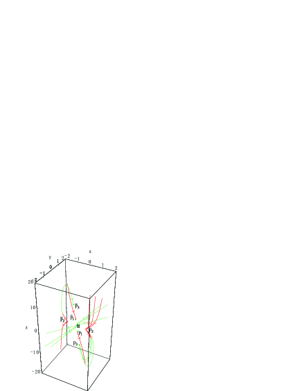
Figure 10: Solution space and flow in the case with a dynamical dilaton. The solid (red) lines correspond to $d^{2}a/d\tau^{2}>0$ and the dashed (green) lines correspond to $d^{2}a/d\tau^{2}<0$.

When we consider the accelerating expansion of the present universe, the fine-tuning problem is always a nagging problem. To partially answer this question, we have examined solutions by changing initial conditions near the fixed point P₂, and find that there are several solutions flowing into P₂, as shown in Fig. 10. This means that there are certain range of initial conditions which lead to the accelerating expansion. In this sense, these solutions have the possibility of explaining naturalness of the accelerating expansion. To examine how large area of these initial conditions can give such a behavior and whether the present model can give realistic one need further study.

5 Conclusions

In this paper we have investigated cosmological solutions in the Einstein theory with GB correction with and without a dilaton in higher dimensions. We are interested in this theory because this is the low-energy effective theory of the heterotic string, and examined what solutions are possible by the dynamical system method. For flat internal and external spaces, we have shown that the field equations can be written as an autonomous system for both the theories with and without dynamical dilaton. We obtained the fixed points and analyzed their stability. We have found that both in the GB correction with and without dilaton, there are solutions with accelerating expansion. Some of them are super-inflation with future singularity.

The analysis in Ref. AH indicates that even if there is no interesting cosmological solution in the Einstein theory for flat internal and external spaces, there may exist an interesting solution with eternally accelerating expansion for curved spaces. The existence of such a solution was originally suggested in Ref. chen by a perturbation around non-inflationary solution, and it was shown that the solution is eternally expanding with acceleration after some time. However, due to the limitation of the perturbation, the detailed properties of the solution (like its eternal accelerating property for whole time) was not clear. The powerful method of dynamical system allowed to show that the solution is eternally expanding with acceleration for the whole time. [21] It is thus possible that similarly interesting solutions may exist in our Einstein-Gauss-Bonnet gravity coupled to dilaton. It would be very interesting to extend our analysis to curved external and internal spaces, and check if there may be additional interesting solutions.

References

-
[1]
D. N. Spergel et al. [WMAP Collaboration],
Astrophys. J. Suppl. 148 (2003) 175
[arXiv:astro-ph/0302209];
Astrophys. J. Suppl. 170 (2007) 377
[arXiv:astro-ph/0603449];
H. V. Peiris et al. [WMAP Collaboration], Astrophys. J. Suppl. 148 (2003) 213 [arXiv:astro-ph/0302225]. - [2] P. K. Townsend and M. N. R. Wohlfarth, Phys. Rev. Lett. 91 (2003) 061302 [arXiv:hep-th/0303097].
- [3] N. Ohta, Phys. Rev. Lett. 91 (2003) 061303 [arXiv:hep-th/0303238]; Prog. Theor. Phys. 110 (2003) 269 [arXiv:hep-th/0304172].
- [4] M. N. R. Wohlfarth, Phys. Lett. B 563 (2003) 1 [arXiv:hep-th/0304089].
-
[5]
C. M. Chen, D. V. Gal’tsov and M. Gutperle,
Phys. Rev. D 66 (2002) 024043
[arXiv:hep-th/0204071];
N. Ohta, Phys. Lett. B 558 (2003) 213 [arXiv:hep-th/0301095]. -
[6]
L. Cornalba and M. S. Costa,
Phys. Rev. D 66 (2002) 066001
[arXiv:hep-th/0203031];
C. P. Burgess, F. Quevedo, S. J. Rey, G. Tasinato and I. Zavala, JHEP 0210 (2002) 028 [arXiv:hep-th/0207104];
S. Roy, Phys. Lett. B 567 (2003) 322 [arXiv:hep-th/0304084];
A. Buchel and J. Walcher, JHEP 0305 (2003) 069 [arXiv:hep-th/0305055];
C. Armendariz-Picon and V. Duvvuri, Class. Quant. Grav. 21 (2004) 2011 [arXiv:hep-th/0305237];
C. P. Burgess, P. Martineau, F. Quevedo, G. Tasinato and I. Zavala C., JHEP 0303 (2003) 050 [arXiv:hep-th/0301122];
I. P. Neupane and D. L. Wiltshire, Phys. Lett. B 619 (2005) 201 [arXiv:hep-th/0502003]; Phys. Rev. D 72 (2005) 083509 [arXiv:hep-th/0504135]. -
[7]
L. Cornalba and M. S. Costa,
Fortsch. Phys. 52 (2004) 145
[arXiv:hep-th/0310099];
V. Balasubramanian, Class. Quant. Grav. 21 (2004) S1337 [arXiv:hep-th/0404075];
N. Ohta, Int. J. Mod. Phys. A 20 (2005) 1 [arXiv:hep-th/0411230]. - [8] C. M. Chen, P. M. Ho, I. P. Neupane, N. Ohta and J. E. Wang, JHEP 0310 (2003) 058 [arXiv:hep-th/0306291]; JHEP 0611 (2006) 044 [arXiv:hep-th/0609043].
- [9] S. Kachru, R. Kallosh, A. Linde, J. M. Maldacena, L. McAllister and S. P. Trivedi, JCAP 0310 (2003) 013 [arXiv:hep-th/0308055].
- [10] A. A. Starobinsky, Phys. Lett. B 91 (1980) 99.
- [11] D. J. Gross and J. H. Sloan, Nucl. Phys. B 291 (1987) 41.
- [12] M. de Roo, H. Suelmann and A. Wiedemann, Nucl. Phys. B 405 (1993) 326 [arXiv:hep-th/9210099].
- [13] A. A. Tseytlin, Nucl. Phys. B 467 (1996) 383 [arXiv:hep-th/9512081].
- [14] K. Peeters, P. Vanhove and A. Westerberg, Class. Quant. Grav. 18 (2001) 843 [arXiv:hep-th/0010167].
- [15] H. Ishihara, Phys. Lett. B 179 (1986) 217.
-
[16]
K. Maeda,
Phys. Lett. B 166 (1986) 59;
B. C. Paul and S. Mukherjee, Phys. Rev. D 42 (1990) 2595;
M. Gasperini and M. Giovannini, Phys. Lett. B 287 (1992) 56. - [17] M. H. Dehghani, Phys. Rev. D 70 (2004) 064009.
-
[18]
S. Nojiri, S. D. Odintsov and M. Sasaki,
Phys. Rev. D 71 (2005) 123509
[arXiv:hep-th/0504052];
G. Calcagni, S. Tsujikawa and M. Sami, Class. Quant. Grav. 22 (2005) 3977 [arXiv:hep-th/0505193];
S. Nojiri, S. D. Odintsov and M. Sami, Phys. Rev. D 74 (2006) 046004 [arXiv:hep-th/0605039];
S. Tsujikawa, Annalen Phys. 15 (2006) 302 [arXiv:hep-th/0606040];
T. Koivisto and D. F. Mota, Phys. Lett. B 644 (2007) 104 [arXiv:astro-ph/0606078]; Phys. Rev. D 75 (2007) 023518 [arXiv:hep-th/0609155];
K. Andrew, B. Bolen and C. A. Middleton, arXiv:hep-th/0608127;
S. Tsujikawa and M. Sami, JCAP 0701 (2007) 006 [arXiv:hep-th/0608178];
S. Nojiri and S. D. Odintsov, arXiv:hep-th/0611071;
G. Cognola et al., Phys. Rev. D 75 (2007) 086002 [arXiv:hep-th/0611198];
E. Elizalde et al.,Phys. Lett. B 644 (2007) 1 [arXiv:hep-th/0611213];
B. M. Leith and I. P. Neupane, JCAP 0705 (2007) 019 [arXiv:hep-th/0702002];
L. Amendola, C. Charmousis and S. C. Davis, arXiv:0704.0175 [astro-ph];
A. Sheykhi, B. Wang and N. Riazi, Phys. Rev. D 75 (2007) 123513 [arXiv:0704.0666];
S. Nojiri, S. D. Odintsov and P. V. Tretyakov, arXiv:0704.2520;
E. Elizalde et al., arXiv:0705.1211;
F. Canfora, A. Giacomini and S. Willison, arXiv:0706.2891. - [19] Z. K. Guo, N. Ohta and S. Tsujikawa, Phys. Rev. D 75 (2007) 023520 [arXiv:hep-th/0610336].
-
[20]
K. Maeda and N. Ohta,
Phys. Lett. B 597 (2004) 400
[arXiv:hep-th/0405205];
Phys. Rev. D 71 (2005) 063520
[arXiv:hep-th/0411093];
K. Akune, K. Maeda and N. Ohta, Phys. Rev. D 73 (2006) 103506 [arXiv:hep-th/0602242]. - [21] L. Andersson and J. M. Heinzle, arXiv:hep-th/0602102.
- [22] J. Sonner and P. K. Townsend, Phys. Rev. D 74 (2006) 103508 [arXiv:hep-th/0608068].
-
[23]
Y. S. Piao and E. Zhou,
Phys. Rev. D 68 (2003) 083515
[arXiv:hep-th/0308080];
Y. S. Piao and Y. Z. Zhang, Phys. Rev. D 70 (2004) 063513 [arXiv:astro-ph/0401231];
Z. K. Guo, Y. S. Piao and Y. Z. Zhang, Phys. Lett. B 594 (2004) 247 [arXiv:astro-ph/0404225].