IPM/P-2007/049 Double Lepton Polarization in $\Lambda_{b}\rightarrow\Lambda\ell^{+}\ell^{-}$ Decay in the Standard Model with Fourth Generations Scenario

This study investigates the influence of the fourth generation quarks on the double lepton polarizations in $\Lambda_{b}\rightarrow\Lambda\ell^{+}\ell^{-}$ decay by taking $|V^{\ast}_{t^{\prime}s}V_{t^{\prime}b}|=0.005,0.01,0.02,0.03$ with phase $\{60^{\circ},90^{\circ},120^{\circ}\}$. We will try to obtain a constrain on the mass of the 4th generation top like quark $t^{\prime}$, which is consistent with the $b\to s\ell^{+}\ell^{-}$ rate . With the above mentioned parameters, we will try to show that the double lepton($\mu,\,\tau$) polarizations are quite sensitive to the existence of fourth generation. It can serve as a good tool to search for new physics effects, precisely, to search for the fourth generation quarks($t^{\prime},\,b^{\prime})$ via its indirect manifestations in loop diagrams.

PACS numbers: 12.60.–i, 13.30.–a, 14.20.Mr

1 Introduction

While the Standard Model (SM) provides a very good description of phenomena observed by experiments, it is still an incomplete theory. The problem is that the Standard Model can’t explain why some particles exist as they do. Another question concerns the fact that there are 3 pairs of quarks and 3 pairs of leptons. Each ”set” of these particles is called a generation (a.k.a. family). Therefore, the up/down quarks are first generation quarks, while the electron and e–neutrino are first generation leptons. In the every-day world we observe only the first-generation particles (electrons, e- neutrinos, and up/down quarks). Why does the natural world, ”need” the two other generations? Are there 3 generations or more? Nothing in the standard model itself fixes the number of quarks and leptons that can exist. Since the first three generations are full, any new quarks and leptons would be members of a ”fourth generation”. In this sense, SM may be treated as an effective theory of fundamental interactions rather than fundamental particles. The Democratic Mass Matrix approach [1], which is quite natural in the SM framework, may be considered as the interesting step in true direction. It is intriguing that Flavors Democracy favors the existence of the fourth SM family [2, 3, 4]. Any study related to the decay of the 4th generation quarks or indirect effects of those in FCNC requires the choice of the quark masses which are not free parameter, rather they are constrained by the experimental value of $\rho$ and $S$ parameters [4]. The $\rho$ parameter, in terms of the transverse part of the W–and Z–boson self energies at zero momentum transfer, is given in [5],

$$\rho=\frac{1}{1-\Delta\rho};\,\,\ \Delta\rho=\frac{\Pi_{ZZ}(0)}{M_{Z}^{2}}-\frac{\Pi_{WW}(0)}{M_{W}^{2}},$$ (1)

the common mass of the fourth generation quarks ($m_{t^{\prime}}$) lies between 320 GeV and 730 GeV considering the experimental value of $\rho=1.0002^{+0.0007}_{-0.0004}$ [6]. The last value is close to upper limit on heavy quark mass, $m_{q}\leq 700$ GeV $\approx 4m_{t}$, which follows from partial-wave unitarity at high energies [7]. It should be noted that with preferable value $a\approx g_{w}$, Flavor Democracy predicts $m_{t^{\prime}}\approx 8m_{w}\approx 640$ GeV. The above mentioned values for mass of $m_{t^{\prime}}$ disfavors the fifth SM family both because in general we expect that $m_{t}\leq m_{t^{\prime}}\leq m_{t}^{{}^{\prime\prime}}$ and the experimental values of the $\rho$ and $S$ parameters [4] restrict the quark mass up to $700$ GeV.

The study of production, decay channels and LHC signals of the 4th generation quarks have been continuing. But, one of the efficient ways to establish the existence of 4th generation is via their indirect manifestations in loop diagrams. Rare decays, induced by flavor changing neutral current (FCNC) $b\rightarrow s(d)$ transitions are at the forefront of our quest to understand flavor and the origins of CPV, offering one of the best probes for New Physics (NP) beyond the Standard Model (SM). Several hints for NP have emerged in the past few years. For example, a large difference is seen in direct CP asymmetries in $B\to K\pi$ decays [8],

$${\cal A}_{K\pi}\equiv A_{\rm CP}(B^{0}\to K^{+}\pi^{-})=-0.093\pm 0.015,$$

$${\cal A}_{K\pi^{0}}\equiv A_{\rm CP}(B^{+}\to K^{+}\pi^{0})=+0.047\pm 0.026,$$ (2)

or $\Delta{\cal A}_{K\pi}\equiv{\cal A}_{K\pi^{0}}-{\cal A}_{K\pi}=(14\pm 3)\%$ [9]. As this percentage was not predicted when first measured in 2004, it has stimulated discussion on the potential mechanisms that it may have been missed in the SM calculations [10, 11, 12].

Better known is the mixing-induced CP asymmetry ${\cal S}_{f}$ measured in a multitude of CP eigenstates $f$. For penguin-dominated $b\to sq\bar{q}$ modes, within SM, ${\cal S}_{sq\bar{q}}$ should be close to that extracted from $b\to c\bar{c}s$ modes. The latter is now measured rather precisely, ${\cal S}_{c\bar{c}s}=\sin 2\phi_{1}=0.674\pm 0.026$ [13], where $\phi_{1}$ is the weak phase in $V_{td}$. However, for the past few years, data seem to indicate at 2.6$\,\sigma$ significance,

$$\Delta{\cal S}\equiv{\cal S}_{sq\bar{q}}-{\cal S}_{c\bar{c}s}\leq 0,$$ (3)

which has stimulated even more discussions.

The $b\rightarrow s(d)\ell^{+}\ell^{-}$ decays have received considerable attention as a potential testing ground for the effective Hamiltonian describing FCNC in B and $\Lambda_{b}$ decay. This Hamiltonian contains the one–loop effects of the electroweak interaction, which are sensitive to the quark^,s contribution in the loop [14]–[16]. In addition, there are important QCD corrections, which have recently been calculated in the NNLL[17]. Moreover, $b\rightarrow s(d)\ell^{+}\ell^{-}$ decay is also very sensitive to the new physics beyond SM. New physics effects manifest themselves in rare decays in two different ways, either through new combinations to the new Wilson coefficients or through the new operator structure in the effective Hamiltonian, which is absent in the SM. A crucial problem in the new physics search within flavour physics is the optimal separation of new physics effects from uncertainties. It is well known that inclusive decay modes are dominated by partonic contributions; non–perturbative corrections are in general rather small[18]. Also ratios of exclusive decay modes such as asymmetries for $B\rightarrow K(~{}K^{\ast},~{}\rho,~{}\gamma)~{}\ell^{+}\ell^{-}$ decay [19]–[27] are well studied for new physics search. Here large parts of the hadronic uncertainties partially cancel out. In this paper, we investigate the possibility of searching for new physics in the heavy baryon decays $\Lambda_{b}\rightarrow\Lambda\ell^{+}\ell^{-}$ using the SM with four generations of quarks($b^{\prime},\,t^{\prime}$). The fourth quark ($t^{\prime}$), like $u,c,t$ quarks, contributes in the $b\rightarrow s(d)$ transition at loop level. Note that, fourth generation effects have been widely studied in baryonic and semileptonic B decays [28]–[41]. But, there are few works related to the exclusive decays $\Lambda_{b}\rightarrow\Lambda l^{+}l^{-}$[42].

The main problem for the description of exclusive decays is to evaluate the form factors, i.e., matrix elements of the effective Hamiltonian between initial and final hadron states. It is well known that in order to describe baryonic $\Lambda_{b}\rightarrow\Lambda\ell^{+}\ell^{-}$ decay a number of form factors are needed (see for example [43]). However, when heavy quark effective theory (HQET) is applied, only two independent form factors appear [44].

It should be mentioned here that for the exclusive decay $\Lambda_{b}\rightarrow\Lambda\ell^{+}\ell^{-}$, decay rate, lepton polarization and heavy($\Lambda_{b}$) or light($\Lambda$) baryon polarization(readily measurable) are studied in the SM, the two Higgs doublet model and using the general form of the effective Hamiltonian, in [43], [45] and [46]–[49], respectively.

The sensitivity of the forward–backward asymmetry to the existence of fourth generation quarks in the $\Lambda_{b}\rightarrow\Lambda\ell^{+}\ell^{-}$ decay is investigated in [41] and it is obtained that the forward–backward asymmetry is very sensitive to the fourth generation parameters ($m_{t^{\prime}}$, $V_{t^{\prime}b}V^{*}_{t^{\prime}s}$ ). In this connection, it is natural to ask whether double lepton polarizations are sensitive to the fourth generation parameters, in the ”heavy baryon $\rightarrow$ light baryon $\ell^{+}\ell^{-}$” decays. In the present work, we try to answer to this question.

The paper is organized as follows: In section 2, using the effective hamiltonian, the general expressions for the matrix element of $\Lambda_{b}\rightarrow\Lambda\ell^{+}\ell^{-}$ decay is derived. Section 3 devoted to the calculations of double–lepton polarizations. In section 4, we investigate the sensitivity of these functions to the fourth generation parameters ($m_{t^{\prime}}$, $r_{sb},\,\ \phi_{sb}$ ).

2 Strategy

We first consider the standard model contribution. In the SM, the matrix element of the $\Lambda_{b}\rightarrow\Lambda\ell^{+}\ell^{-}$ decay at quark level is described by $b\rightarrow s\ell^{+}\ell^{-}$ transition for which the effective Hamiltonian at $O(\mu)$ scale can be written as:

$${\cal H}_{eff} = \frac{4G_{F}}{\sqrt{2}}V_{tb}V_{ts}^{\ast}\sum_{i=1}^{10}{\cal C}_{i}(\mu)\,{\cal O}_{i}(\mu)~{},$$ (4)

where the full set of the operators ${\cal O}_{i}(\mu)$ and the corresponding expressions for the Wilson coefficients ${\cal C}_{i}(\mu)$ in the SM are given in [50]–[52]. As it has already been noted , the fourth generation up type quark $t^{\prime}$ is introduced in the same way as $u,\ c,\ t$ quarks introduce in the SM, and so new operators do not appear and clearly the full operator set is exactly the same as in SM. The fourth generation changes the values of the Wilson coefficients $C_{7}(\mu),~{}C_{9}(\mu)$ and $C_{10}(\mu)$, via virtual exchange of the fourth generation up type quark $t^{\prime}$. The above mentioned Wilson coefficients will explicitly change as:

$$\lambda_{t}C_{i}\rightarrow\lambda_{t}C^{SM}_{i}+\lambda_{t^{\prime}}C^{new}_{i}~{},$$ (5)

where $\lambda_{f}=V_{fb}^{\ast}V_{fs}$. The unitarity of the $4\times 4$ CKM matrix leads to

$$\lambda_{u}+\lambda_{c}+\lambda_{t}+\lambda_{t^{\prime}}=0.$$ (6)

Since $\lambda_{u}=V_{ub}^{\ast}V_{us}$ is very small in strength compared to the others . Then $\lambda_{t}\approx-\lambda_{c}-\lambda_{t^{\prime}}$ and $\lambda_{c}=V_{cb}^{\ast}V_{cs}\approx 0.04$ is real by convention. It follows that

$$\lambda_{t}C^{SM}_{i}+\lambda_{t^{\prime}}C^{new}_{i}=\lambda_{c}C^{SM}_{i}+\lambda_{t^{\prime}}(C^{new}_{i}-C^{SM}_{i})$$ (7)

It is clear that, for the $m_{t^{\prime}}\rightarrow m_{t}$ or $\lambda_{t^{\prime}}\rightarrow 0$, $\lambda_{t^{\prime}}(C^{new}_{i}-C^{SM}_{i})$ term vanishes, as required by the GIM mechanism. One can also write $C_{i}$’s in the following form

$$C_{7}^{tot}(\mu) = C_{7}^{SM}(\mu)+\frac{\lambda_{t^{\prime}}}{\lambda_{t}}C_{7}^{new}(\mu)~{},$$

$$C_{9}^{tot}(\mu) = C_{9}^{SM}(\mu)+\frac{\lambda_{t^{\prime}}}{\lambda_{t}}C_{9}^{new}(\mu)~{},$$

$$C_{10}^{tot}(\mu) = C_{10}^{SM}(\mu)+\frac{\lambda_{t^{\prime}}}{\lambda_{t}}C_{10}^{new}(\mu)~{},$$ (8)

where the last terms in these expressions describe the contributions of the $t^{\prime}$ quark to the Wilson coefficients. $\lambda_{t^{\prime}}$ can be parameterized as :

$${}\lambda_{t^{\prime}}=V_{t^{\prime}b}^{\ast}V_{t^{\prime}s}=r_{sb}e^{i\phi_{sb}}$$ (9)

In deriving Eq. (2) we factored out the term $V_{tb}^{\ast}V_{ts}$ in the effective Hamiltonian given in Eq. (4). The explicit forms of the $C_{i}^{new}$ can easily be obtained from the corresponding expression of the Wilson coefficients in SM by substituting $m_{t}\rightarrow m_{t^{\prime}}$ (see [50, 51]). If the $s$ quark mass is neglected, the above effective Hamiltonian leads to following matrix element for the $b\rightarrow s\ell^{+}\ell^{-}$ decay

$${\cal H}_{eff} = \frac{G\alpha}{2\sqrt{2}\pi}V_{tb}V_{ts}^{\ast}\Bigg{[}C_{9}^{tot}\,\bar{s}\gamma_{\mu}(1-\gamma_{5})b\,\bar{\ell}\gamma_{\mu}\ell+C_{10}^{tot}\bar{s}\gamma_{\mu}(1-\gamma_{5})b\,\bar{\ell}\gamma_{\mu}\gamma_{5}\ell$$ (10)

$$- 2C_{7}^{tot}\frac{m_{b}}{q^{2}}\bar{s}\sigma_{\mu\nu}q^{\nu}(1+\gamma_{5})b\,\bar{\ell}\gamma_{\mu}\ell\Bigg{]}~{},$$

where $q^{2}=(p_{1}+p_{2})^{2}$ and $p_{1}$ and $p_{2}$ are the final leptons four–momenta. The effective coefficient $C_{9}^{tot}$ can be written in the following form

$$C_{9}^{tot}=C_{9}+Y(s^{\prime})~{},$$ (11)

where $s^{\prime}=q^{2}/m_{b}^{2}$ and the function $Y(s^{\prime})$ denotes the perturbative part coming from one loop matrix elements of four quark operators and is given[50, 52],

$$Y_{per}(s^{\prime}) = g(\hat{m}_{c},s^{\prime})(3C_{1}+C_{2}+3C_{3}+C_{4}+3C_{5}+C_{6})$$ (12)

$$- \frac{1}{2}g(1,s^{\prime})(4C_{3}+4C_{4}+3C_{5}+C_{6})$$

$$- \frac{1}{2}g(0,s^{\prime})(C_{3}+3C_{4})+\frac{2}{9}(3C_{3}+C_{4}+3C_{5}+C_{6})~{},$$

where $\hat{m}_{c}=\frac{m_{c}}{m_{b}}$. The explicit expressions for $g(\hat{m}_{c},s^{\prime})$, $g(0,s^{\prime})$, $g(1,s^{\prime})$ and the values of $C_{i}$ in the SM can be found in Table 1 [50, 52].

$$\begin{array}[]{|c|c|c|c|c|c|c|c|c|}\hline\cr C_{1}&C_{2}&C_{3}&C_{4}&C_{5}&C_{6}&C_{7}^{SM}&C_{9}^{SM}&C_{10}^{SM}\\ \hline\cr-0.248&1.107&0.011&-0.026&0.007&-0.031&-0.313&4.344&-4.669\\ \hline\cr\end{array}$$

Table 1: The numerical values of the Wilson coefficients at $\mu=m_{b}$ scale within the SM. The corresponding numerical value of $C_{0}$ is $0.362$.

In addition to the short distance contribution, $Y_{per}(s^{\prime})$ receives also long distance contributions, which have their origin in the real $c\bar{c}$ intermediate states, i.e., $J/\psi$, $\psi^{\prime}$, $\cdots$. The $J/\psi$ family is introduced by the Breit–Wigner distribution for the resonances through the replacement [53]–[55]

$$Y(s^{\prime})=Y_{per}(s^{\prime})+\frac{3\pi}{\alpha^{2}}\,C^{(0)}\sum_{V_{i}=\psi_{i}}\kappa_{i}\,\frac{m_{V_{i}}\Gamma(V_{i}\rightarrow\ell^{+}\ell^{-})}{m_{V_{i}}^{2}-s^{\prime}m_{b}^{2}-im_{V_{i}}\Gamma_{V_{i}}}~{},$$ (13)

where $C^{(0)}=3C_{1}+C_{2}+3C_{3}+C_{4}+3C_{5}+C_{6}$. The phenomenological parameters $\kappa_{i}$ can be fixed from ${\cal B}(B\rightarrow K^{\ast}V_{i}\rightarrow K^{\ast}\ell^{+}\ell^{-})={\cal B}(B\rightarrow K^{\ast}V_{i})\,{\cal B}(V_{i}\rightarrow\ell^{+}\ell^{-})$, where the data for the right hand side is given in [56]. For the lowest resonances $J/\psi$ and $\psi^{\prime}$ one can use $\kappa=1.65$ and $\kappa=2.36$, respectively (see [57]).

After having an idea of the effective Hamiltonian and the relevant Wilson coefficients, we now proceed to evaluate the transition matrix elements for the process $\Lambda_{b}(p_{\Lambda_{b}})\to\Lambda(p_{\Lambda})~{}l^{+}(p_{+})l^{-}(p_{-})$. For this purpose, we need to know the marix elements of the various hadronic currents between initial $\Lambda_{b}$ and the final $\Lambda$ baryon, which are parameterized in terms of various form factors as

$$\langle\Lambda|\bar{s}\gamma_{\mu}b|\Lambda_{b}\rangle = \bar{u}_{\Lambda}\Big{[}f_{1}\gamma_{\mu}+if_{2}\sigma_{\mu\nu}q^{\nu}+f_{3}q_{\mu}\Big{]}u_{\Lambda_{b}}\;,$$ (14)

$$\langle\Lambda|\bar{s}\gamma_{\mu}\gamma_{5}b|\Lambda_{b}\rangle = \bar{u}_{\Lambda}\Big{[}g_{1}\gamma_{\mu}\gamma_{5}+ig_{2}\sigma_{\mu\nu}\gamma_{5}q^{\nu}+g_{3}\gamma_{5}q_{\mu}\Big{]}u_{\Lambda_{b}}\;,$$ (15)

$$\langle\Lambda|\bar{s}i\sigma_{\mu\nu}q^{\nu}b|\Lambda_{b}\rangle = \bar{u}_{\Lambda}\Big{[}f_{1}^{T}\gamma_{\mu}+if_{2}^{T}\sigma_{\mu\nu}q^{\nu}+f_{3}^{T}q_{\mu}\Big{]}u_{\Lambda_{b}}\;,$$ (16)

$$\langle\Lambda|\bar{s}i\sigma_{\mu\nu}\gamma_{5}q^{\nu}b|\Lambda_{b}\rangle = \bar{u}_{\Lambda}\Big{[}g_{1}^{T}\gamma_{\mu}\gamma_{5}+ig_{2}^{T}\sigma_{\mu\nu}\gamma_{5}q^{\nu}+g_{3}^{T}\gamma_{5}q_{\mu}\Big{]}u_{\Lambda_{b}}\;,$$ (17)

where $q=p_{\Lambda_{b}}-p_{\Lambda}=p_{+}+p_{-}$ is the momentum transfer, $f_{i}$ and $g_{i}$ are the various form factors which are functions of $q^{2}$. The number of independent form factors are greatly reduced in the heavy quark symmetry limit. In this limit, the matrix elements of all the hadronic currents, irrespective of their Dirac structure, can be given in terms of only two independent form factors [46] as

$$\langle\Lambda(p_{\Lambda})|\bar{s}\Gamma b|\Lambda_{b}(p_{\Lambda_{b}})\rangle=\bar{u}_{\Lambda}[F_{1}(q^{2})+\not\!{v}F_{2}(q^{2})]\Gamma u_{\Lambda_{b}}\;,$$ (18)

where $\Gamma$ is the product of Dirac matrices, $v^{\mu}=p_{\Lambda_{b}}^{\mu}/m_{\Lambda_{b}}$ is the four velocity of $\Lambda_{b}$. These two sets of form facors are relalated to each other as

$$g_{1}=f_{1}=f_{2}^{T}=g_{2}^{T}=F_{1}+\sqrt{r}F_{2}\;,$$ (19)

$$g_{2}=f_{2}=g_{3}=f_{3}=\frac{F_{2}}{m_{\Lambda_{b}}}\;,$$ (20)

$$g_{3}^{T}=\frac{F_{2}}{m_{\Lambda_{b}}}(m_{\Lambda_{b}}+m_{\Lambda})\;,~{}~{}~{}~{}~{}~{}f_{3}^{T}=-\frac{F_{2}}{m_{\Lambda_{b}}}(m_{\Lambda_{b}}-m_{\Lambda})$$ (21)

$$f_{1}^{T}=g_{1}^{T}=\frac{F_{2}}{m_{\Lambda_{b}}}q^{2}\;,$$ (22)

where $r=m_{\Lambda}^{2}/m_{\Lambda_{b}}^{2}$. Thus, using these form factors, the transition amplitude can be written as

$${\cal M}=\frac{G\alpha}{4\sqrt{2}\pi}V_{tb}V_{ts}^{\ast}\Bigg{\{}\bar{\ell}\gamma^{\mu}\ell\,\bar{u}_{\Lambda}\Big{[}A_{1}\gamma_{\mu}(1+\gamma_{5})+B_{1}\gamma_{\mu}(1-\gamma_{5})$$ (23)

$$+ \!\!\!i\sigma_{\mu\nu}q^{\nu}\big{[}A_{2}(1+\gamma_{5})+B_{2}(1-\gamma_{5})\big{]}+q_{\mu}\big{[}A_{3}(1+\gamma_{5})+B_{3}(1-\gamma_{5})\big{]}\Big{]}u_{\Lambda_{b}}$$

$$+ \!\!\!\bar{\ell}\gamma^{\mu}\gamma_{5}\ell\,\bar{u}_{\Lambda}\Big{[}E_{1}\gamma_{\mu}(1-\gamma_{5})+i\sigma_{\mu\nu}q^{\nu}E_{2}(1-\gamma_{5})+E_{3}q^{\mu}(1-\gamma_{5})\big{]}\Big{]}u_{\Lambda_{b}}\Bigg{\}}~{},$$

where $P=p_{\Lambda_{b}}+p_{\Lambda}$. Explicit expressions of the functions $A_{i},~{}B_{i},$ and $E_{i}$ $(i=1,2,3)$ are given as follows [46]:

$$A_{1} = -\frac{4m_{b}}{m_{\Lambda_{b}}}~{}F_{2}~{}C^{tot}_{7}$$

$$A_{2} = -\frac{4m_{b}}{q^{2}}~{}(F_{1}+\sqrt{r}F_{2})~{}C^{tot}_{7}$$

$$A_{3} = -\frac{4m_{b}m_{\Lambda}}{q^{2}m_{\Lambda_{b}}}~{}F_{2}~{}C^{tot}_{7}$$

$$B_{1} = 2(F_{1}+\sqrt{r}F_{2})~{}C^{tot}_{9}$$

$$B_{2} = \frac{2F_{2}}{m_{\Lambda_{b}}}~{}C^{tot}_{9}$$

$$B_{3} = \frac{4m_{b}}{q^{2}}~{}F_{2}~{}C^{tot}_{7}$$

$$E_{1} = 2(F_{1}+\sqrt{r}F_{2})~{}C^{tot}_{10}$$

$$E_{2} = E_{3}=\frac{2F_{2}}{m_{\Lambda_{b}}}~{}C^{tot}_{10}$$ (24)

From the expressions of the above-mentioned matrix elements Eq. (23) we observe that $\Lambda_{b}\rightarrow\Lambda\ell^{+}\ell^{-}$ decay is described in terms of many form factors. When HQET is applied to the number of independent form factors, as it has already been noted, reduces to two ($F_{1}$ and $F_{2}$) irrelevant with the Dirac structure of the corresponding operators and it is obtained in [44] that

$$\left<\Lambda(p_{\Lambda})\left|\bar{s}\Gamma b\right|\Lambda(p_{\Lambda_{b}})\right>=\bar{u}_{\Lambda}\Big{[}F_{1}(q^{2})+\not\!vF_{2}(q^{2})\Big{]}\Gamma u_{\Lambda_{b}}~{},$$ (25)

where $\Gamma$ is an arbitrary Dirac structure, $v^{\mu}=p_{\Lambda_{b}}^{\mu}/m_{\Lambda_{b}}$ is the four–velocity of $\Lambda_{b}$, and $q=p_{\Lambda_{b}}-p_{\Lambda}$ is the momentum transfer. Comparing the general form of the form factors with (2), one can easily obtain the following relations among them (see also [43])

$$g_{1}\!\!\! = \!\!\!f_{1}=f_{2}^{T}=g_{2}^{T}=F_{1}+\sqrt{r}F_{2}~{},$$

$$g_{2}\!\!\! = \!\!\!f_{2}=g_{3}=f_{3}=g_{T}^{V}=f_{T}^{V}=\frac{F_{2}}{m_{\Lambda_{b}}}~{},$$

$$g_{T}^{S}\!\!\! = \!\!\!f_{T}^{S}=0~{},$$

$$g_{1}^{T}\!\!\! = \!\!\!f_{1}^{T}=\frac{F_{2}}{m_{\Lambda_{b}}}q^{2}~{},$$

$$g_{3}^{T}\!\!\! = \!\!\!\frac{F_{2}}{m_{\Lambda_{b}}}\left(m_{\Lambda_{b}}+m_{\Lambda}\right)~{},$$

$$f_{3}^{T}\!\!\! = \!\!\!-\frac{F_{2}}{m_{\Lambda_{b}}}\left(m_{\Lambda_{b}}-m_{\Lambda}\right)~{},$$ (26)

where $r=m_{\Lambda}^{2}/m_{\Lambda_{b}}^{2}$.

The differential decay rate of the $\Lambda_{b}\rightarrow\Lambda\ell^{+}\ell^{-}$ decay for any spin direction can be written as:

$$\left(\frac{d\Gamma}{ds}\right)_{0}=\frac{G^{2}\alpha^{2}}{192\pi^{5}}\left|V_{tb}V_{ts}^{\ast}\right|^{2}\lambda^{1/2}(1,r,s)v\Big{[}{\cal T}_{0}(s)+\frac{1}{3}{\cal T}_{2}(s)\Big{]}~{},$$ (27)

where $\lambda(1,r,s)=1+r^{2}+s^{2}-2r-2s-2rs$ is the triangle function and $v=\sqrt{1-4m_{\ell}^{2}/q^{2}}$ is the lepton velocity. The explicit expressions for ${\cal T}_{0}$ and ${\cal T}_{2}$ are given by:

$${\cal T}_{0} = 4m_{\Lambda_{b}}^{2}\Big{\{}8m_{\ell}^{2}m_{\Lambda_{b}}^{2}\hat{s}(1+r-\hat{s})|E_{3}|^{2}+16m_{\ell}^{2}m_{\Lambda_{b}}\sqrt{r}(1-r+\hat{s})\mbox{\rm Re}[E_{1}^{\ast}E_{3}]+$$ (28)

$$8(2m_{\ell}^{2}+m_{\Lambda_{b}}^{2}\hat{s})\{(1-r+\hat{s})m_{\Lambda_{b}}\sqrt{r}\mbox{\rm Re}[A_{1}^{\ast}A_{2}+B_{1}^{\ast}B_{2}]-$$

$$m_{\Lambda_{b}}(1-r-\hat{s})\mbox{\rm Re}[A_{1}^{\ast}B_{2}+A_{2}^{\ast}B_{1}]-2\sqrt{r}(\mbox{\rm Re}[A_{1}^{\ast}B_{1}]+m_{\Lambda_{b}}^{2}\hat{s}\mbox{\rm Re}[A_{2}^{\ast}B_{2}])\}+$$

$$2\Big{(}4m_{\ell}^{2}(1+r-\hat{s})+m_{\Lambda_{b}}^{2}\Big{[}(1-r)^{2}-\hat{s}^{2}\Big{]}\Big{)}\Big{(}|A_{1}|^{2}+|B_{1}|^{2}\Big{)}+$$

$$2m_{\Lambda_{b}}^{2}\Big{(}4m_{\ell}^{2}\Big{[}\lambda+(1+r-\hat{s})\hat{s}\Big{]}+m_{\Lambda_{b}}^{2}\hat{s}\Big{[}(1-r)^{2}-\hat{s}^{2}\Big{]}\Big{)}\Big{(}|A_{2}|^{2}+|B_{2}|^{2}\Big{)}-$$

$$2\Big{(}4m_{\ell}^{2}(1+r-\hat{s})-m_{\Lambda_{b}}^{2}\Big{[}(1-r)^{2}-\hat{s}^{2}\Big{]}\Big{)}|E_{1}|^{2}+$$

$$2m_{\Lambda_{b}}^{3}\hat{s}v^{2}\Big{(}4(1-r+\hat{s})\sqrt{r}\mbox{\rm Re}[E_{1}^{\ast}E_{2}]-m_{\Lambda_{b}}\Big{[}(1-r)^{2}-\hat{s}^{2}\Big{]}|E_{2}|^{2}\Big{)}\Big{\}}$$

$${\cal T}_{2}=-8m_{\Lambda_{b}}^{4}v^{2}\lambda\Big{(}|A_{1}|^{2}+|B_{1}|^{2}+|E_{1}|^{2}-m_{\Lambda_{b}}^{2}\hat{s}(|A_{2}|^{2}+|B_{2}|^{2}+|E_{2}|^{2})\Big{)}.$$ (29)

3 Double–lepton polarization asymmetries in the $\Lambda_{b}\rightarrow\Lambda\ell^{+}\ell^{-}$ decay

In order to calculate the polarization asymmetries of both leptons defined in the effective four fermion interaction of Eq.(23), we must first define the orthogonal vectors $S$ in the rest frame of $\ell^{-}$ and $W$ in the rest frame of $\ell^{+}$ (where these vectors are the polarization vectors of the leptons). Note that we shall use the subscripts $L$, $N$ and $T$ to correspond to the leptons being polarized along the longitudinal, normal and transverse directions respectively [58, 59].

$$S^{\mu}_{L} \equiv (0,\mathbf{e}_{L})~{}=~{}\left(0,\frac{\mathbf{p}_{-}}{|\mathbf{p}_{-}|}\right),$$

$$S^{\mu}_{N} \equiv (0,\mathbf{e}_{N})~{}=~{}\left(0,\frac{\mathbf{p_{\Lambda}}\times\mathbf{p}_{-}}{|\mathbf{p_{\Lambda}}\times\mathbf{p}_{-}|}\right),$$

$$S^{\mu}_{T} \equiv (0,\mathbf{e}_{T})~{}=~{}\left(0,\mathbf{e}_{N}\times\mathbf{e}_{L}\right),$$ (30)

$$W^{\mu}_{L} \equiv (0,\mathbf{w}_{L})~{}=~{}\left(0,\frac{\mathbf{p}_{+}}{|\mathbf{p}_{+}|}\right),$$

$$W^{\mu}_{N} \equiv (0,\mathbf{w}_{N})~{}=~{}\left(0,\frac{\mathbf{p_{\Lambda}}\times\mathbf{p}_{+}}{|\mathbf{p_{\Lambda}}\times\mathbf{p}_{+}|}\right),$$

$$W^{\mu}_{T} \equiv (0,\mathbf{w}_{T})~{}=~{}(0,\mathbf{w}_{N}\times\mathbf{w}_{L}),$$ (31)

where $\mathbf{p}_{+}$, $\mathbf{p}_{-}$ and $\mathbf{p_{\Lambda}}$ are the three momenta of the $\ell^{+}$, $\ell^{-}$ and $\Lambda$ particles respectively. On boosting the vectors defined by Eqs.(30,31) to the c.m. frame of the $\ell^{-}\ell^{+}$ system only the longitudinal vector will be boosted, whilst the other two vectors remain unchanged. The longitudinal vectors after the boost will become;

$$S^{\mu}_{L} = \left(\frac{|\mathbf{p}_{-}|}{m_{\ell}},\frac{E_{\ell}\mathbf{p}_{-}}{m_{\ell}|\mathbf{p}_{-}|}\right),$$

$$W^{\mu}_{L} = \left(\frac{|\mathbf{p}_{-}|}{m_{\ell}},-\frac{E_{\ell}\mathbf{p}_{-}}{m_{\ell}|\mathbf{p}_{-}|}\right).$$ (32)

The polarization asymmetries can now be calculated using the spin projector ${1\over 2}(1+\gamma_{5}\!\!\not\!\!S)$ for $\ell^{-}$ and the spin projector ${1\over 2}(1+\gamma_{5}\!\not\!\!W)$ for $\ell^{+}$.

Equipped with the above expressions we now define the various double lepton polarization asymmetries. The double lepton polarization asymmetries are defined as [59];

$${\cal P}_{xy} \equiv \frac{\left(\frac{d\Gamma(S_{x},W_{y})}{d\hat{s}}-\frac{d\Gamma(-S_{x},W_{y})}{d\hat{s}}\right)-\left(\frac{d\Gamma(S_{x},-W_{y})}{d\hat{s}}-\frac{d\Gamma(-S_{x},-W_{y})}{d\hat{s}}\right)}{\left(\frac{d\Gamma(S_{x},W_{y})}{d\hat{s}}+\frac{d\Gamma(-S_{x},W_{y})}{d\hat{s}}\right)+\left(\frac{d\Gamma(S_{x},-W_{y})}{d\hat{s}}+\frac{d\Gamma(-S_{x},-W_{y})}{d\hat{s}}\right)},$$ (33)

where the sub-indices $x$ and $y$ can be either $L$, $N$ or $T$. And the double polarization asymmetries are;

$$P_{LL} = \frac{8m^{4}_{\Lambda_{b}}}{3\Delta}Re\Bigg{\{}12\hat{m}_{\ell}(1-\sqrt{\hat{r}_{\Lambda}})(1+2\sqrt{\hat{r}_{\Lambda}}+\hat{r}_{\Lambda}-\hat{s})E_{1}F_{2}^{\ast}$$

$$+ 3\hat{s}(1+2\sqrt{\hat{r}_{\Lambda}}+\hat{r}_{\Lambda}-\hat{s})[v^{2}|F_{1}|^{2}+|F_{2}|^{2}+4m_{\Lambda_{b}}\hat{m}_{\ell}F_{3}F_{2}^{\ast}]$$

$$- 12m_{\Lambda_{b}}\sqrt{\hat{r}_{\Lambda}}(1-\hat{r}_{\Lambda}+\hat{s})[\hat{s}(1+v^{2})(A_{1}A_{2}^{\ast}+B_{1}B_{2}^{\ast})-4\hat{m}_{\ell}^{2}E_{1}E_{3}^{\ast}]$$

$$+ 12m_{\Lambda_{b}}(1-\hat{r}_{\Lambda}-\hat{s})[\hat{s}(1+v^{2})(A_{1}B_{2}^{\ast}+A_{2}B_{1}^{\ast})]$$

$$+ 24\sqrt{\hat{r}_{\Lambda}}\hat{s}(1+v^{2})(A_{1}B_{1}^{\ast}+m_{\Lambda_{b}}^{2}\hat{s}A_{2}B_{2}^{\ast})+24m_{\Lambda_{b}}^{2}\hat{m}_{\ell}^{2}\hat{s}(1+\hat{r}_{\Lambda}-\hat{s})|E_{3}|^{2}$$

$$- 2(1+v^{2})[1+\hat{r}_{\Lambda}^{2}-\hat{r}_{\Lambda}(2-\hat{s})+\hat{s}(1-2\hat{s})](|A_{1}|^{2}+|B_{1}|^{2})$$

$$- 2[(5v^{2}-3)(1-\hat{r}_{\Lambda})^{2}+4\hat{m}_{\ell}^{2}(1+\hat{r}_{\Lambda})+2\hat{s}(1+8\hat{m}_{\ell}^{2}+\hat{r}_{\Lambda})-4\hat{s}^{2}]|E_{1}|^{2}$$

$$- 2m_{\Lambda_{b}}^{2}(1+v^{2})\hat{s}[2+2\hat{r}_{\Lambda}^{2}-\hat{s}(1+\hat{s})-\hat{r}_{\Lambda}(4+\hat{s})](|A_{2}|^{2}+|B_{2}|^{2})$$

$$- 4m_{\Lambda_{b}}^{2}\hat{s}v^{2}[2(1+\hat{r}_{\Lambda}^{2})-\hat{s}(1+\hat{s})-\hat{r}_{\Lambda}(4+\hat{s})]|E_{2}|^{2}$$

$$- 24m_{\Lambda_{b}}\sqrt{\hat{r}_{\Lambda}}\hat{s}(1-\hat{r}_{\Lambda}+\hat{s})v^{2}E_{1}E_{2}^{\ast}\Bigg{\}}$$

$$P_{NL}=-P_{LN} = \frac{4\pi m^{4}_{\Lambda_{b}}\sqrt{\lambda}}{\Delta\sqrt{\hat{s}}}Im\Bigg{\{}4\hat{m}_{\ell}(1-\hat{r}_{\Lambda})B_{1}^{\ast}E_{1}+4m_{\Lambda_{b}}\hat{m}_{\ell}\hat{s}(A_{1}^{\ast}E_{3}-A_{2}^{\ast}E_{1})$$

$$+ \hat{s}(1+\sqrt{\hat{r}_{\Lambda}})(A_{1}+B_{1})^{\ast}F_{2}+4m_{\Lambda_{b}}\hat{m}_{\ell}\sqrt{\hat{r}_{\Lambda}}\hat{s}(B_{1}^{\ast}E_{3}+B_{2}^{\ast}E_{1})$$

$$- m_{\Lambda_{b}}\hat{s}^{2}[B_{2}^{\ast}(F_{2}+4m_{\Lambda_{b}}\hat{m}_{\ell}E_{3})+A_{2}^{\ast}F_{2}]-\hat{s}v^{2}[E_{1}F_{1}^{\ast}-\sqrt{\hat{r}_{\Lambda}}E_{1}^{\ast}F_{1}]+m_{\Lambda_{b}}\hat{s}^{2}v^{2}F_{1}E_{2}^{\ast}\Bigg{\}}$$

$$P_{TL}=P_{LT} = \frac{4\pi m_{\Lambda_{b}}^{4}\sqrt{\lambda}v}{\Delta\sqrt{\hat{s}}}Re\Bigg{\{}4\hat{m}_{\ell}(1-\hat{r}_{\Lambda})|E_{1}|^{2}-4\hat{m}_{\ell}~{}\hat{s}~{}B_{1}E_{1}^{\ast}$$

$$- 4\hat{m}_{\ell}~{}\hat{s}~{}m_{\Lambda_{b}}(A_{2}E_{1}^{\ast}-A_{1}E_{2}^{\ast})-\hat{s}(1+\sqrt{\hat{r}_{\Lambda}})[(A_{1}+B_{1})F_{1}^{\ast}-E_{1}F_{2}^{\ast}]$$

$$- 4m_{\Lambda_{b}}^{2}\hat{s}(1-\hat{r}_{\Lambda})\hat{m}_{\ell}B_{2}E_{2}^{\ast}-4m_{\Lambda_{b}}\hat{m}_{\ell}\sqrt{\hat{r}_{\Lambda}}\hat{s}[B_{1}E_{2}^{\ast}+(B_{2}-E_{2}-E_{3})E_{1}^{\ast}]$$

$$+ m_{\Lambda_{b}}\hat{s}^{2}[(A_{2}+B_{2})F_{1}^{\ast}-E_{2}F_{2}^{\ast}-4m_{\Lambda_{b}}\hat{m}_{\ell}E_{2}E_{3}^{\ast}]\Bigg{\}}$$

$$P_{NT} = \frac{16m_{\Lambda_{b}}^{4}v}{3\Delta}Im\Bigg{\{}4\lambda B_{1}E_{1}^{\ast}-6\hat{m}_{\ell}(1-\sqrt{\hat{r}_{\Lambda}})(1+2\sqrt{\hat{r}_{\Lambda}}+\hat{r}_{\Lambda}-\hat{s})E_{1}F_{1}^{\ast}$$

$$+ 4m_{\Lambda_{b}}^{2}\lambda\hat{s}E_{2}B_{2}^{\ast}-3\hat{s}(1+2\sqrt{\hat{r}_{\Lambda}}+\hat{r}_{\Lambda}-\hat{s})(F_{2}+2m_{\Lambda_{b}}\hat{m}_{\ell}E_{3})F_{1}^{\ast}\Bigg{\}}$$

$$P_{TN} = -\frac{16m_{\Lambda_{b}}^{4}v}{3\Delta}Im\Bigg{\{}4\lambda B_{1}E_{1}^{\ast}+6\hat{m}_{\ell}(1-\sqrt{\hat{r}_{\Lambda}})(1+2\sqrt{\hat{r}_{\Lambda}}+\hat{r}_{\Lambda}-\hat{s})E_{1}F_{1}^{\ast}$$

$$+ 4m_{\Lambda_{b}}^{2}\lambda\hat{s}E_{2}B_{2}^{\ast}+3\hat{s}(1+2\sqrt{\hat{r}_{\Lambda}}+\hat{r}_{\Lambda}-\hat{s})(F_{2}+2m_{\Lambda_{b}}\hat{m}_{\ell}E_{3})F_{1}^{\ast}\Bigg{\}}$$

$$P_{NN} = \frac{8m^{4}_{\Lambda_{b}}}{3\hat{s}\Delta}Re\Bigg{\{}96\hat{m}_{l}^{2}\sqrt{\hat{r_{\Lambda}}}\hat{s}A_{1}B_{1}^{\ast}$$

$$- 48m_{\Lambda_{b}}\hat{m}_{l}^{2}\sqrt{\hat{r_{\Lambda}}}\hat{s}(1-\hat{r}_{\Lambda}+\hat{s})(A_{1}A_{2}^{\ast}+B_{1}B_{2}^{\ast})$$

$$+ 12\hat{m}_{l}\hat{s}(1-\sqrt{\hat{r}_{\Lambda}})(1+2\sqrt{\hat{r}_{\Lambda}}+\hat{r}_{\Lambda}-\hat{s})E_{1}F_{2}^{\ast}$$

$$+ 3\hat{s}^{2}(1+2\sqrt{\hat{r}_{\Lambda}}+\hat{r}_{\Lambda}-\hat{s})[|F_{2}|^{2}+4m_{\Lambda_{b}}\hat{m}_{l}E_{3}F_{2}^{\ast}]$$

$$+ 24m_{\Lambda_{b}}\hat{m}_{l}^{2}\hat{s}[m_{\Lambda_{b}}\hat{s}(1+\hat{r}_{\Lambda}-\hat{s})|E_{3}|^{2}+2\sqrt{\hat{r}_{\Lambda}}(1-\hat{r}_{\Lambda}+\hat{s})E_{1}E_{3}^{\ast}]$$

$$+ 48m_{\Lambda_{b}}\hat{m}_{l}^{2}\hat{s}(1-\hat{r}_{\Lambda}-\hat{s})(A_{1}B_{2}^{\ast}+A_{2}B_{1}^{\ast})$$

$$- 4[\lambda\hat{s}+2\hat{m}_{l}^{2}(1+\hat{r}_{\Lambda}^{2}-2\hat{r}_{\Lambda}+\hat{r}_{\Lambda}\hat{s}+\hat{s}-2\hat{s}^{2})](|A_{1}|^{2}+|B_{1}|^{2}-|E_{1}|^{2})$$

$$+ 96m_{\Lambda_{b}}^{2}\hat{m}_{l}^{2}\sqrt{\hat{r_{\Lambda}}}\hat{s}^{2}A_{2}B_{2}^{\ast}-4m_{\Lambda_{b}}^{2}\lambda\hat{s}^{2}v^{2}|E_{2}|^{2}$$

$$+ 4m_{\Lambda_{b}}^{2}\hat{s}\{\lambda\hat{s}-2\hat{m}_{l}^{2}[2(1+\hat{r}^{2})-\hat{s}(1+\hat{s})-\hat{r}(4+\hat{s})]\}(|A_{2}|^{2}+|B_{2}|^{2})$$

$$- 3\hat{s}^{2}v^{2}(1+2\sqrt{\hat{r_{\Lambda}}}+\hat{r_{\Lambda}}-\hat{s})|F_{1}|^{2}\Bigg{\}}$$

$$P_{TT} = \frac{8m^{4}_{\Lambda_{b}}}{3\hat{s}\Delta}Re\Bigg{\{}-96\hat{m}_{l}^{2}\sqrt{\hat{r_{\Lambda}}}\hat{s}A_{1}B_{1}^{\ast}$$

$$- 48m_{\Lambda_{b}}\hat{m}_{l}^{2}\sqrt{\hat{r_{\Lambda}}}\hat{s}(1-\hat{r}_{\Lambda}+\hat{s})E_{1}E_{3}^{\ast}$$

$$- 12\hat{m}_{l}\hat{s}(1-\sqrt{\hat{r}_{\Lambda}})(1+2\sqrt{\hat{r}_{\Lambda}}+\hat{r}_{\Lambda}-\hat{s})E_{1}F_{2}^{\ast}$$

$$- 96m_{\Lambda_{b}}^{2}\hat{m}_{l}^{2}\sqrt{\hat{r_{\Lambda}}}\hat{s}^{2}A_{2}B_{2}^{\ast}-3\hat{s}^{2}(1+2\sqrt{\hat{r}_{\Lambda}}+\hat{r}_{\Lambda}-\hat{s})[|F_{2}|^{2}+4m_{\Lambda_{b}}\hat{m}_{l}E_{3}F_{2}\ast]$$

$$- 24m_{\Lambda_{b}}\hat{m}_{l}^{2}\hat{s}[m_{\Lambda_{b}}\hat{s}(1+\hat{r}_{\Lambda}-\hat{s})|E_{3}|^{2}-2\sqrt{\hat{r}_{\Lambda}}(1-\hat{r}_{\Lambda}+\hat{s})(A_{1}A_{2}^{\ast}+B_{1}B_{2}^{\ast})]$$

$$- 48m_{\Lambda_{b}}\hat{m}_{l}^{2}\hat{s}(1-\hat{r}_{\Lambda}-\hat{s})(A_{1}B_{2}^{\ast}+A_{2}B_{1}^{\ast})$$

$$- 4[\lambda\hat{s}-2\hat{m}_{l}^{2}(1+\hat{r}_{\Lambda}^{2}-2\hat{r}_{\Lambda}+\hat{r}_{\Lambda}\hat{s}+\hat{s}-2\hat{s}^{2})](|A_{1}|^{2}+|B_{1}|^{2})$$

$$+ 4m_{\Lambda_{b}}^{2}\hat{s}\{\lambda\hat{s}+\hat{m}_{l}^{2}[4(1-\hat{r}_{\Lambda})^{2}-2\hat{s}(1+\hat{r}_{\Lambda})-2\hat{s}^{2}]\}(|A_{2}|^{2}+|B_{2}|^{2})$$

$$+ 4\{\lambda\hat{s}-2\hat{m}_{l}^{2}[5(1-\hat{r}_{\Lambda})^{2}-v\hat{s}(1+\hat{r}_{\Lambda})+2\hat{s}^{2}]\}|E_{1}|^{2}$$

$$- 4m_{\Lambda_{b}}^{2}\lambda\hat{s}^{2}v^{2}|E_{2}|^{2}+3\hat{s}^{2}v^{2}(1+2\sqrt{\hat{r}_{\Lambda}}+\hat{r}_{\Lambda}-\hat{s})|F_{1}|^{2}\Bigg{\}}$$

4 Numerical analysis

In this section, we examine the dependence of the double lepton polarizations to the fourth quark mass($m_{t^{\prime}}$) and the product of quark mixing matrix elements ($V_{t^{\prime}b}^{\ast}V_{t^{\prime}s}=r_{sb}e^{i\phi_{sb}}$). For numerical evaluation we use the various particle masses and lifetimes of $\Lambda_{b}$ baryon from [6]. The quark masses (in GeV) used are $m_{b}$=4.8, $m_{c}$=1.35, the CKM matrix elements as $|V_{cb}V_{cs}^{*}|=0.041$, $\alpha=1/128$ and the weak mixing angle $\sin^{2}\theta_{W}=0.23$. For the form factors we use the values calculated in the QCD sum rule approach in combination with HQET [44, 60], which reduces the number of quite many form factors into two. The $s$ dependence of these form factors can be represented in the following way

$$F(q^{2})=\frac{F(0)}{\displaystyle 1-a_{F}s+b_{F}s^{2}}~{},$$

where parameters $F_{i}(0),~{}a$ and $b$ are listed in table 2.

$$\begin{array}[]{|l|ccc|}\hline\cr&F(0)&a_{F}&b_{F}\\ \hline\cr F_{1}&\phantom{-}0.462&-0.0182&-0.000176\\ F_{2}&-0.077&-0.0685&\phantom{-}0.00146\\ \hline\cr\end{array}$$

Table 2: Transition form factors for $\Lambda_{b}\rightarrow\Lambda\ell^{+}\ell^{-}$ decay in the QCD sum rules method.

We use the next–to–leading order logarithmic approximation for the resulting values of the Wilson coefficients $C_{9}^{eff},~{}C_{7}$ and $C_{10}$ in the SM [61, 62] at the re–normalization point $\mu=m_{b}$. It should be noted that, in addition to short distance contribution, $C_{9}^{eff}$ receives also long distance contributions from the real $\bar{c}c$ resonant states of the $J/\psi$ family. In the present work, we do not take the long distance effects into account. In order to perform quantitative analysis of the double lepton polarizations, the values of the new parameters($m_{t^{\prime}},\,r_{sb},\,\phi_{sb}$) are needed. Using the experimental values of $B\rightarrow X_{s}\gamma$ and $B\rightarrow X_{s}\ell^{+}\ell^{-}$, the bound on $r_{sb}\sim\{0.01-0.03\}$ has been obtained [33] for $\phi_{sb}\sim\{0-2\pi\}$ and $m_{t^{\prime}}\sim\{300,400\}~{}$(GeV). We do a different and somehow more general analysis with the recent world average value[17] of the

$${\cal{B}}(B\rightarrow X_{s}\ell^{+}\ell^{-})=(1.6\pm 0.51)\times 10^{-6},\,\,\,\,\,\ell=(\mu,\,e)$$ (41)

in the low dilepton invariant mass region($1\texttt{GeV}^{2}<q^{2}<6\texttt{GeV}^{2}$). We chose $r_{sb}\sim\{0.005-0.03\}$ , $\phi_{sb}\sim\{60^{\circ}-120^{\circ}\}$ and $1\sigma$ level deviation from the experimental value, then we obtain the constrain on $m_{t^{\prime}}$ (see Table 3, 4 and 5 ). However, the most general analysis about range of new parameters ($\phi_{sb},~{}r_{sb},m_{t^{\prime}}$) considering the recent experimental value of $B\rightarrow X_{s}\ell^{+}\ell^{-}$ are still incomplete in some sense. We plan to do that in our next work. In the foregoing numerical analysis, we vary $m_{t^{\prime}}$ in the range $175\leq m_{t^{\prime}}\leq 600$GeV. The lower range is because of the fact that the fourth generation up quark should be heavier than the third ones($m_{t}\leq m_{t^{\prime}}$)[4]. The upper range comes from the experimental bounds on the $\rho$ and $S$ parameters of SM, which we mentioned above(see Introduction). At the same time we will show the constrain on $m_{t^{\prime}}$ coming from the experimental values of the $B\rightarrow X_{s}\ell^{+}\ell^{-}$ in our figures.

Before performing numerical analysis, few words about lepton polarizations are in order. From explicit expressions of the lepton polarizations one can easily see that they depend on both $\hat{s}$ and the new parameters($m_{t^{\prime}},\,r_{sb}$). We should eliminate the dependence of the lepton polarization on one of the variables. We eliminate the variable $\hat{s}$ by performing integration over $\hat{s}$ in the allowed kinematical region. The total branching ratio and the averaged lepton polarizations are defined as

$${\cal B}_{r} = \displaystyle\int_{4m_{\ell}^{2}/m_{\Lambda_{b}}^{2}}^{(1-\sqrt{r})^{2}}\frac{d{\cal B}}{ds}ds,$$

$$\left<P_{ij}\right> = \frac{\displaystyle\int_{4m_{\ell}^{2}/m_{\Lambda_{b}}^{2}}^{(1-\sqrt{r})^{2}}P_{ij}\frac{d{\cal B}}{ds}ds}{{\cal{B}}_{r}}~{}.$$ (42)

We ignore to show $\left<P_{LL}\right>$ for the $\Lambda_{b}\rightarrow\Lambda\mu^{+}\mu^{-}$ decay, since its value is quite small.

Figs. (1)–(33) show the dependency of $\left<P_{ij}\right>$ for the $\Lambda_{b}\rightarrow\Lambda\ell^{+}\ell^{-}$ decay at four values of $r_{sb}:0.005,0.01,0.02,0.03$ on the $m_{t^{\prime}}$ for $\ell=\mu,\,\tau$ channels at three different values of $\phi_{sb}:60^{\circ},90^{\circ}120^{\circ}$. The $\bullet\!\!\!\backslash$ sign in figures show the experimental upper limit on $m_{t^{\prime}}$ coming from the $B\rightarrow X_{s}\ell^{+}\ell^{-}$ analysis. From these figures, we obtain the following results.

$$\begin{array}[]{|c|c|c|c |c|}\hline\cr r_{sb}&0.005&0.01&0.02&0.03\\ \hline\cr m_{t^{\prime}}(GeV)&739&529&385&331\\ \hline\cr\end{array}$$

Table 3: The extracted maximum experimental limit of $m_{t^{\prime}}$ for $\phi_{sb}=\pi/3$

$$\begin{array}[]{|c|c|c|c |c|}\hline\cr r_{sb}&0.005&0.01&0.02&0.03\\ \hline\cr m_{t^{\prime}}(GeV)&511&373&289&253\\ \hline\cr\end{array}$$

Table 4: The extracted maximum experimental limit of $m_{t^{\prime}}$ for $\phi_{sb}=\pi/2$

$$\begin{array}[]{|c|c|c|c |c|}\hline\cr r_{sb}&0.005&0.01&0.02&0.03\\ \hline\cr m_{t^{\prime}}(GeV)&361&283&235&217\\ \hline\cr\end{array}$$

Table 5: The extracted maximum experimental limit of $m_{t^{\prime}}$ for $\phi_{sb}=2\pi/3$

• $\left<P_{LL}\right>$ for $\Lambda_{b}\rightarrow\Lambda\tau^{+}\tau^{-}$ decay depends strongly on the SM4 parameters. Firstly, there exist regions of the $m_{t^{\prime}}$ where $\left<P_{LL}\right>$ departs considerably from the SM3 result. Secondly, there is an experimentally allowed regions for the value of $m_{t^{\prime}}$ where $\left<P_{LL}\right>$ changes its sign(see Fig. 1)in compare with SM3 value. The measurement of the sign of $\left<P_{LL}\right>$ for $\tau$ channel can be used as a good tool to look for new Physics effects. More precisely, the results can be used to indirect search to look for fourth generation of quarks.

• $\left<P_{LN}\right>$($\left<P_{NL}\right>$)and $\left<P_{TN}\right>$(-$\left<P_{NT}\right>$) show strong dependency on SM4 parameters. It is increasing function in the experimentally allowed regions and decreasing function of $\phi_{sb}$ for both $\mu$ and $\tau$ channels(see Figs. 4–9 and Figs. 22–27). The SM3 values of $\left<P_{LN}\right>$($\left<P_{NL}\right>$)and $\left<P_{TN}\right>$(-$\left<P_{NT}\right>$) approximately vanish for both . But, it receive the maximum values of $\approx 0.1$ , $\approx 0.4$ and $\approx 0.4$ and minimum value $\approx-0.1$ for $\mu$ and $\tau$ channels(see Figs. 4, 5 and Figs. 22, 25), respectively. The results can be used to look for NP. It should be noted that, when $m_{t^{\prime}}\rightarrow m_{t}$ the SM4 result could coincide with the SM3 (see Strategy). The deviation of $\approx 1\%$ from the SM3 values for $\mu$ channel(see Figs. 4, 6, 8 and 25–27) is because, firstly, we use the NNLL calculation for the SM3 values of Wilson coefficients($C_{i}^{SM}$) and LL formulas for $C_{i}^{new}$(see Eq. (2)). Secondly, our numerical integration for $P_{ij}$ has the same order of error.

• $\left<P_{LT}\right>$($\left<P_{TL}\right>$) are very sensitive to $m_{t^{\prime}}$ and $r_{sb}$ and less sensitive to the $\phi_{sb}$. We observe that $\left<P_{LT}\right>$($\left<P_{TL}\right>$) exceeds the SM3 prediction 2 and 3 times for $\mu$ and $\tau$ channels(see Figs. 10–15), respectively. Such behaviors can serve as a good test for establishing new physics beyond the SM.

• $\left<P_{TT}\right>$ and $\left<P_{NN}\right>$ are quite sensitive to the existence of the SM4 parameters either in experimentally allowed regions or in the hole region. They are increasing and decreasing function of $m_{t^{\prime}}$ if $\phi_{sb}=60^{\circ}$. But, they are just increasing for $\mu$ case and decreasing for $\tau$ case if $\phi_{sb}=90^{\circ}$ or $\phi_{sb}=120^{\circ}$. In the presence of the 4th generation, the magnitude of $\left<P_{TT}\right>$ can exceed the SM result 8 and 2 times and $\left<P_{NN}\right>$ can exceed the SM result 4 and 5 times for $\mu$ and $\tau$ cases, respectively. Therefore, determination of the magnitude of $\left<P_{TT}\right>$ and $\left<P_{NN}\right>$ can give unambiguous information about the existence of the new generation.

At the end of this section, let us discuss the problem of measurement of the lepton polarization asymmetries in experiments. Experimentally, to measure an asymmetry $\langle P_{ij}\rangle$ of the decay with the branching ratio ${\cal B}$ at $n\sigma$ level, the required number of events (i.e., the number of $B\bar{B}$ pair) are given by the expression

$$N=\frac{n^{2}}{{\cal B}s_{1}s_{2}\langle P_{ij}\rangle^{2}}~{},$$

where $s_{1}$ and $s_{2}$ are the efficiencies of the leptons. Typical values of the efficiencies of the $\tau$–leptons range from $50\%$ to $90\%$ for their various decay modes (see for example [63] and references therein), and the error in $\tau$–lepton polarization is estimated to be about $(10-15)\%$ [64]. As a result, the error in measurement of the $\tau$–lepton asymmetries is of the order of $(20-30)\%$, and the error in obtaining the number of events is about $50\%$.

From the expression for $N$ we see that, in order to observe the lepton polarization asymmetries in $\Lambda_{b}\rightarrow\Lambda\mu^{+}\mu^{-}$ and $\Lambda_{b}\rightarrow\Lambda\tau^{+}\tau^{-}$ decays at $3\sigma$ level, the minimum number of required events are (for the efficiency of $\tau$–lepton we take $0.5$):

• for the $\Lambda_{b}\rightarrow\Lambda\mu^{+}\mu^{-}$ decay

  $$N=\left\{\begin{array}[]{ll}2.0\times 10^{6}&(\mbox{\rm for}\left<P_{LL}\right>)~{},\\ 2.0\times 10^{8}&(\mbox{\rm for}\left<P_{LT}\right>=\left<P_{TL}\right>,\left<P_{NN}\right>,\left<P_{TT}\right>)~{},\end{array}\right.$$ (45)

• for $\Lambda_{b}\rightarrow\Lambda\tau^{+}\tau^{-}$ decay

  $$N=\left\{\begin{array}[]{ll}(4.0\pm 2)\times 10^{9}&(\mbox{\rm for}\left<P_{LT}\right>,\left<P_{NN}\right>)~{},\\ (1.0\pm 0.5)\times 10^{9}&(\mbox{\rm for}\left<P_{TT}\right>)~{},\\ (2.0\pm 1.0)\times 10^{11}&(\mbox{\rm for}\left<P_{LN}\right>,\left<P_{NL}\right>)~{},\\ (9.0\pm 4.5)\times 10^{8}&(\mbox{\rm for}\left<P_{TL}\right>)~{}.\end{array}\right.$$ (50)

The number of $B\bar{B}$ pairs, that are produced at B–factories and LHC   are about $\sim 5\times 10^{8}$ and $10^{12}$, respectively. As a result of a comparison of these numbers and $N$, we conclude that, only $\left<P_{LL}\right>$ in the $\Lambda_{b}\rightarrow\Lambda\mu^{+}\mu^{-}$ decay and $\left<P_{LT}\right>$, $\left<P_{NN}\right>$ and $\left<P_{TL}\right>$ in the $\Lambda_{b}\rightarrow\Lambda\tau^{+}\tau^{-}$ decay, can be detectable at LHC.

To sum up, we presented the most general analysis of the double–lepton polarization asymmetries in the $\Lambda_{b}\rightarrow\Lambda\ell^{+}\ell^{-}$ decay using the SM with fourth generation in this study. We also studied the dependence of the averaged double–lepton polarization asymmetries on the SM4 parameters. Our results showed that the averaged double–lepton polarization asymmetries are strongly dependent on the fourth quark ($m_{t^{\prime}}$) and the product of quark mixing matrix elements ($V_{t^{\prime}b}^{\ast}V_{t^{\prime}s}=r_{sb}e^{i\phi_{sb}}$). Thus, the experimental determination of both the sign and the magnitude of the $\left<P_{ij}\right>$ can serve as a good tool to look for new physics beyond the SM. More precisely, the study of the averaged double–lepton polarization asymmetries can serve as good tool for searching new generation of quarks.

5 Acknowledgment

The authors would like to thank T. M. Aliev for his useful discussions. Also, the authors would like to thank TWAS, Iranian chapter via ISOMO, for their partially support.

Figure captions

Fig. (1) The dependence of $\left<P_{LL}\right>$ for $\Lambda_{b}\rightarrow\Lambda\tau^{+}\tau^{-}$decay on $m_{t^{\prime}}$, at four fixed values of $r_{sb}:0.005,0.01,0.02,0.03$ and $\phi_{sb}=60^{\circ}$ .

Fig. (2) The same as in Fig. (1), but for $\phi_{sb}=90^{\circ}$.

Fig. (3) The same as in Fig. (1), but for $\phi_{sb}=120^{\circ}$.

Fig. (4) The dependence of $\left<P_{LN}\right>$ for $\Lambda_{b}\rightarrow\Lambda\mu^{+}\mu^{-}$decay on $m_{t^{\prime}}$, at four fixed values of $r_{sb}:0.005,0.01,0.02,0.03$ and $\phi_{sb}=60^{\circ}$ .

Fig. (5) The same as in Fig. (4), but for the $\tau$ lepton.

Fig. (6) The same as in Fig. (4), but for $\phi_{sb}=90^{\circ}$.

Fig. (7) The same as in Fig. (6), but for the $\tau$ lepton.

Fig. (8) The same as in Fig. (4), but for $\phi_{sb}=120^{\circ}$.

Fig. (9) The same as in Fig. (8), but for the $\tau$ lepton.

Fig. (10) The dependence of $\left<P_{LT}\right>$ for $\Lambda_{b}\rightarrow\Lambda\mu^{+}\mu^{-}$decay on $m_{t^{\prime}}$, at four fixed values of $r_{sb}:0.005,0.01,0.02,0.03$ and $\phi_{sb}=60^{\circ}$ .

Fig. (11) The same as in Fig. (10), but for the $\tau$ lepton.

Fig. (12) The same as in Fig. (10), but for $\phi_{sb}=90^{\circ}$.

Fig. (13) The same as in Fig. (12), but for the $\tau$ lepton.

Fig. (14) The same as in Fig. (10), but for $\phi_{sb}=120^{\circ}$.

Fig. (15) The same as in Fig. (14), but for the $\tau$ lepton.

Fig. (16) The dependence of $\left<P_{TT}\right>$ for $\Lambda_{b}\rightarrow\Lambda\mu^{+}\mu^{-}$decay on $m_{t^{\prime}}$, at four fixed values of $r_{sb}:0.005,0.01,0.02,0.03$ and $\phi_{sb}=60^{\circ}$ .

Fig. (17) The same as in Fig. (16), but for the $\tau$ lepton.

Fig. (18) The same as in Fig. (16), but for $\phi_{sb}=90^{\circ}$.

Fig. (19) The same as in Fig. (18), but for the $\tau$ lepton.

Fig. (20) The same as in Fig. (16), but for $\phi_{sb}=120^{\circ}$.

Fig. (21) The same as in Fig. (20), but for the $\tau$ lepton.

Fig. (22) The dependence of $\left<P_{TN}\right>$ for $\Lambda_{b}\rightarrow\Lambda\mu^{+}\mu^{-}$decay on $m_{t^{\prime}}$, at four fixed values of $r_{sb}:0.005,0.01,0.02,0.03$ and $\phi_{sb}=60^{\circ}$ .

Fig. (23) The same as in Fig. (22), but for $\phi_{sb}=90^{\circ}$.

Fig. (24) The same as in Fig. (22), but for $\phi_{sb}=120^{\circ}$.

Fig. (25) The dependence of $\left<P_{NT}\right>$ for $\Lambda_{b}\rightarrow\Lambda\tau^{+}\tau^{-}$decay on $m_{t^{\prime}}$, at four fixed values of $r_{sb}:0.005,0.01,0.02,0.03$ and $\phi_{sb}=60^{\circ}$ .

Fig. (26) The same as in Fig. (25), but for $\phi_{sb}=90^{\circ}$.

Fig. (27) The same as in Fig. (25), but for $\phi_{sb}=120^{\circ}$.

Fig. (28) The dependence of $\left<P_{NN}\right>$ for $\Lambda_{b}\rightarrow\Lambda\mu^{+}\mu^{-}$decay on $m_{t^{\prime}}$, at four fixed values of $r_{sb}:0.005,0.01,0.02,0.03$ and $\phi_{sb}=60^{\circ}$ .

Fig. (29) The same as in Fig. (28), but for the $\tau$ lepton.

Fig. (30) The same as in Fig. (28), but for $\phi_{sb}=90^{\circ}$.

Fig. (31) The same as in Fig. (30), but for the $\tau$ lepton.

Fig. (32) The same as in Fig. (28), but for $\phi_{sb}=120^{\circ}$.

Fig. (33) The same as in Fig. (32), but for the $\tau$ lepton.

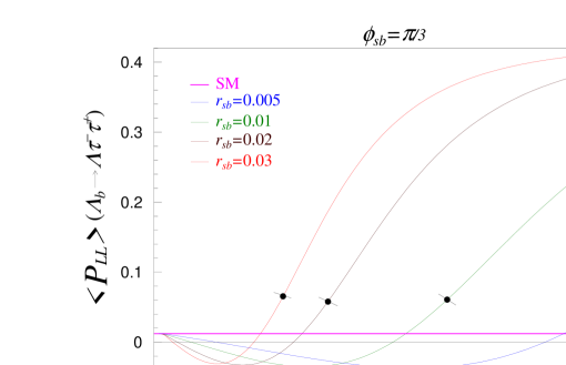
Figure 1:

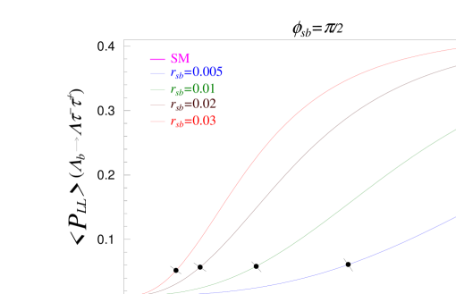
Figure 2:

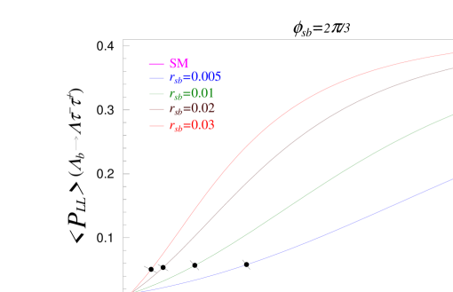
Figure 3:

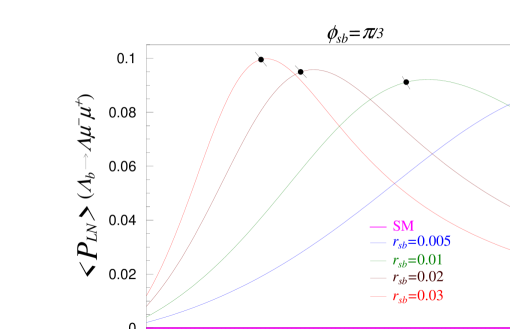
Figure 4:

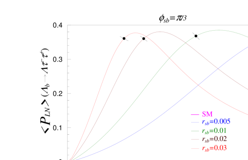
Figure 5:

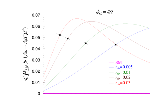
Figure 6:

Figure 7:

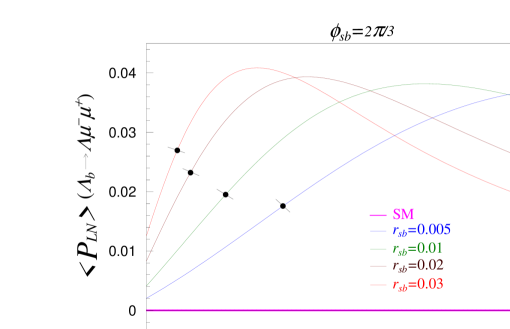
Figure 8:

Figure 9:

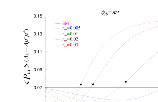
Figure 10:

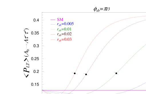
Figure 11:

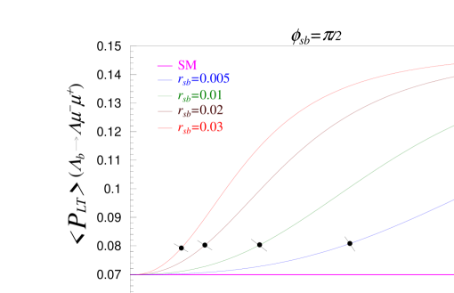
Figure 12:

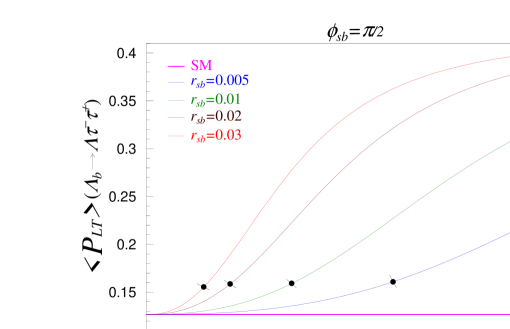
Figure 13:

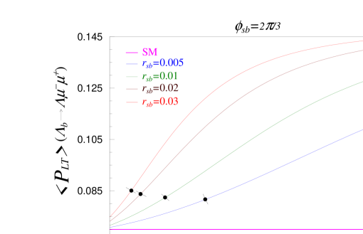
Figure 14:

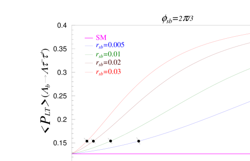
Figure 15:

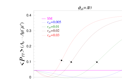
Figure 16:

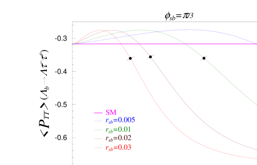
Figure 17:

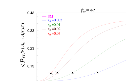
Figure 18:

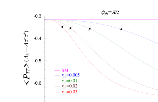
Figure 19:

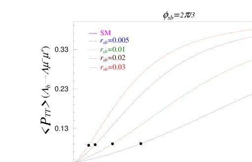
Figure 20:

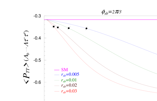
Figure 21:

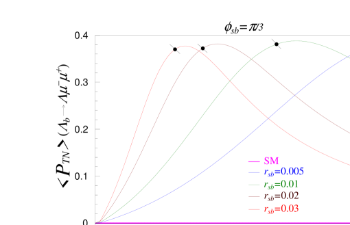
Figure 22:

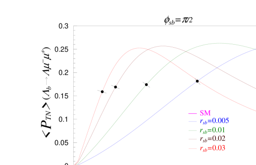
Figure 23:

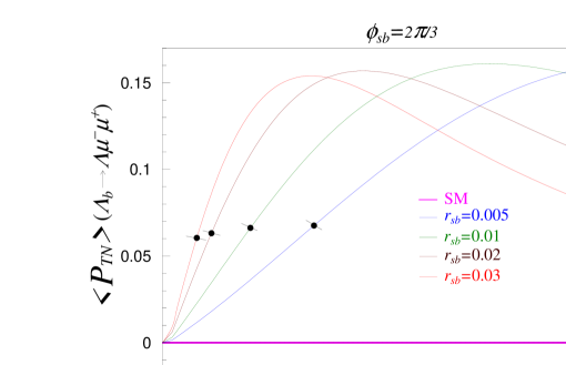
Figure 24:

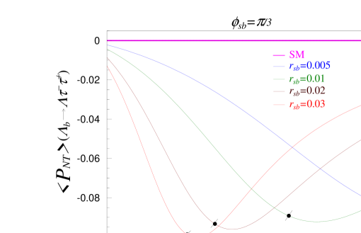
Figure 25:

Figure 26:

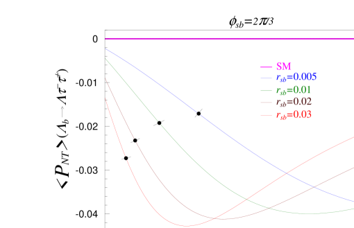
Figure 27:

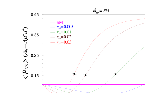
Figure 28:

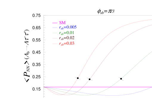
Figure 29:

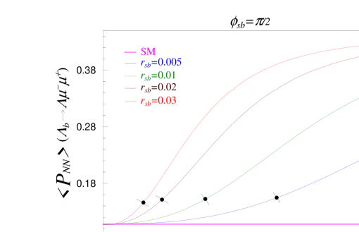
Figure 30:

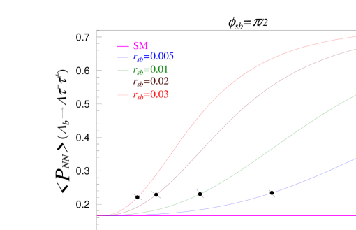
Figure 31:

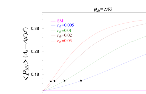
Figure 32:

Figure 33:

References

-
[1]
H. Harari, H. Haut, and J. Weyers
Phys. Lett. B 78 (1978) 459;
H. Fritzch, Nucl. Phys. B 155 (1979) 189; B 184 (1987) 391;
P. Kaus and S. Meshkov, Mod. Phys. Lett. A 3 (1988) 1251;
H. Fritzch and J. Plankl, Phys. Lett. B 237 (1990) 451. - [2] A. Datta, Pramana 40 (1993) L503.
- [3] A. Celikel, A.K. Ciftci and S. Sultansoy, Phys. Lett. B 342 (1995) 257.
- [4] S. Sultansoy, hep-ph/0004271.
- [5] A. Djouadi, P. Gambino, H. Heinemeyer, W. Hollik, C. Junger and G. Weigline, Phys. Rev. Lett 78 (1997) 3626.
- [6] J. Erler and P. Langacker, PDG, J. Phys. G(2006) 130.
- [7] M.S. Chanowitz, M.A. Furlan and I. Hinchliffe, Nucl. Phys. B 153 (1979) 402.
- [8] E. Barberio, (Heavy Flavor Averaging Group), hep-ex/0603003.
- [9] R. Barlow, Plenary talk at 33rd International Conference on High Energy Physics, Moscow, Russia, July 27 - August 2, 2006.
- [10] M. Beneke, G. Buchalla, M. Neubert, and C.T. Sachrajda, Phys. Rev. Lett. 83 (1999) 1914; Nucl. Phys. B 591 (2000) 313; ibid. B 606 (2001) 245.
- [11] Y.Y. Keum, H.N. Li, and A.I. Sanda, Phys Lett. B 504 (2001) 6; Phys. Rev. D 63 (2001) 054008 .
- [12] C.W. Bauer, I.Z. Rothstein and I.W. Stewart, Phys. Rev. D 74 (2006) 034010.
- [13] M. Hazumi, Plenary talk at 33rd International Conference on High Energy Physics, Moscow, Russia, July 27 - August 2, 2006.
- [14] W.S. Hou, R.S. Willey and A. Soni, Phys. Rev. Lett 58 (1987) 1608; ibid 60 (1988) 2337 Erratum.
- [15] N.G. Deshpande and J. Trampetic, Phys. Rev. Lett 60 (1988) 2583.
- [16] A.J. Buras and M. Munez, Phys. Rev. D 52 (1995) 186.
- [17] T. Huber, E. Lunghi, M. Misiak and D. Wyler, Nucl. Phys. B 740 (2006) 105.
- [18] T. Hurth, Rev. Mod. Phys. 75 (2003) 1159.
- [19] J.L. Hewett, Phys. Rev. D 53 (1996) 4964.
- [20] T.M. Aliev, V. Bashiry and M. Savcı, Eur. Phys. J. C 35 (2004) 197.
- [21] T.M. Aliev, V. Bashiry and M. Savcı, Phys. Rev. D 72 (2005) 034031.
- [22] T.M. Aliev, V. Bashiry and M. Savcı, Phys. Rev. D 73 (2006) 034013.
- [23] T.M. Aliev, V. Bashiry and M. Savcı, Eur. Phys. J. C 40 (2005) 505.
- [24] F. Krüger and L.M. Sehgal Phys. Lett. B 380 (1996) 199.
- [25] Y.G. Kim, P. Ko, J.S. Lee, Nucl. Phys. B 544 (1999) 64.
- [26] C.H. Chen and C.Q. Geng, Phys. Lett. B 516 (2001) 327.
- [27] V. Bashiry, Chin. Phys. Lett. 22 (2005) 2201.
- [28] W.S. Hou, H.N. Li, S. Mishima and M. Nagashima, hep-ph/0611107.
- [29] W.S. Hou, M. Nagashima and A. Soddu, Phys. Rev. Lett. 95 (2005) 141601.
- [30] L. solmaz, Phys. Rev. D 69 (2004) 015003.
- [31] W.J. Huo, C.D. Lu and Z.J. Xiao, hep-ph/0302177.
- [32] T.M. Aliev, A. Özpineci and M. Savcı, Eur. Phys. J. C 29 (2003) 265.
- [33] A. Arhrib and W.S. Hou, Eur. Phys. J. C 27 (2003) 555.
- [34] W.J. Huo, hep-ph/0203226.
- [35] T.M. Aliev, A. Özpineci and M. Savcı, Eur. Phys. J. C 27 (2003) 405.
- [36] Y. Dincer, Phys. Lett. B 505 (2001) 89.
- [37] T.M. Aliev, A. Özpineci and M. Savcı, Nucl. Phys. B 585 (2000) 275.
- [38] C.S. Huang, W.J. Huo and Y.L. Wu, Mod. Phys. Lett. A 14 (1999) 2453.
- [39] S. Abachi et al. [D0 Collaboration], Phys. Rev. Lett. 78 (1997) 3818.
- [40] D. London, Phys. Lett. B 234 (1990) 354.
- [41] G. Turan, JHEP 0505 (2005) 008.
- [42] V. Bashiry, K. Azizi, JHEP 07, 064 (2007).
- [43] C.H. Chen and C.Q. Geng, Phys. Rev. D 64 (2001) 074001.
- [44] T. Mannel, W. Roberts and Z. Ryzak, Nucl. Phys. B 355 (1991) 38.
- [45] T.M. Aliev, M. Savcı, J. Phys. G 26 (2000) 997.
- [46] T.M. Aliev, A. Özpineci, M. Savcı, Nucl. Phys. B 649 (2003) 168.
- [47] T.M. Aliev, V. Bashiry and M. Savcı, Eur. Phys. J. C 38 (2004) 283.
- [48] T.M. Aliev, V. Bashiry and M. Savcı, Nucl. Phys. B 709 (2005) 115.
- [49] C.H. Chen and C.Q. Geng, J.N. Ng Phys. Rev. D 65 (2002) 091502.
- [50] A.J. Buras and M. Münz, Phys. Rev. D 52 (1995) 186.
- [51] B. Grinstein, M.J. Savage and M.B. Wise, Nucl. Phys. B 319 (1989) 271.
- [52] M. Misiak, Nucl. Phys. B 393 (1993) 23; Erratum, ibid. B 439 (1995) 461.
- [53] N.G. Deshpande, J. Trampetic and K. Ponose, Phys. Rev. D 39 (1989) 1461.
- [54] C.S. Lim, T. Morozumi and A.I. Sanda, Phys. Lett. B218 (1989) 343.
-
[55]
A.I. Vainshtein, V.I. Zakharov, L.B. Okun,
M. A. Shifman,
Sov. J. Nucl. Phys. 24 (1976) 427. - [56] C. Caso et al., Eur. J. Phys. C 3 (1998) 1.
- [57] A. Ali, P. Ball, L.T. Handoko, G. Hiller, Phys.Rev. D 61 (2000) 074024.
- [58] F. Krüger and L.M. Sehgal, Phys. Lett. B 380 (1996) 199, hep-ph/9603237 . J.L. Hewett, Phys. Rev. D 53 (1996) 4964 , hep-ph/9506289.
- [59] W. Bensalem, D. London, N. Sinha and R. Sinha, Phys. Rev. D 67 (2003) 034007.
- [60] C.S. Huang, H.G. Yan, phys. Rev. D 59 (1999) 114022
- [61] C. Bobeth, M. Misiak, and J. Urban, Nucl. Phys. B 574 (2000) 291.
- [62] H.H. Asatrian, H.M. Asatrian, C. Greub, and M. Walker, Phys. Lett. B 507 (2001) 162.
- [63] G. Abbiendi et. al, OPAL Collaboration, Phys. Lett. B 492 (2000) 23.
- [64] A. Rouge, Workshop on –physics, Orcay, France (1990).