Side-information Scalable Source Coding

Abstract

The problem of side-information scalable (SI-scalable) source coding is considered in this work, where the encoder constructs a progressive description, such that the receiver with high quality side information will be able to truncate the bitstream and reconstruct in the rate distortion sense, while the receiver with low quality side information will have to receive further data in order to decode. We provide inner and outer bounds for general discrete memoryless sources. The achievable region is shown to be tight for the case that either of the decoders requires a lossless reconstruction, as well as the case with degraded deterministic distortion measures. Furthermore we show that the gap between the achievable region and the outer bounds can be bounded by a constant when square error distortion measure is used. The notion of perfectly scalable coding is introduced as both the stages operate on the Wyner-Ziv bound, and necessary and sufficient conditions are given for sources satisfying a mild support condition. Using SI-scalable coding and successive refinement Wyner-Ziv coding as basic building blocks, a complete characterization is provided for the important quadratic Gaussian source with multiple jointly Gaussian side-informations, where the side information quality does not have to be monotonic along the scalable coding order. Partial result is provided for the doubly symmetric binary source with Hamming distortion when the worse side information is a constant, for which one of the outer bound is strictly tighter than the other one.

I Introduction

Consider the following scenario where a server is to broadcast multimedia data to multiple users with different side informations, however the side informations are not available at the server. A user may have such strong side information that only minimal additional information is required from the server to satisfy a fidelity criterion, or a user may have barely any side information and expect the server to provide virtually everything to satisfy a (possibly different) fidelity criterion.

A naive strategy is to form a single description and broadcast it to all the users, who can decode only after receiving it completely regardless of the quality of their individual side informations. However, for the users with good-quality side information (who will simply be referred to as the good users), most of the information received is redundant, which introduces a delay caused simply by the existence of users with poor-quality side informations (referred to as the bad users) in the network. It is natural to ask whether an opportunistic method exists, i.e., whether it is possible to construct a two-layer description, such that the good users can decode with only the first layer, and the bad users receive both the first and the second layer to reconstruct. Moreover, it is of importance to investigate whether such a coding order introduces any performance loss. We call this coding strategy side-information scalable (SI-scalable) source coding, since the scalable coding direction is from the good users to the bad users. In this work, we consider mostly two-layer systems, except the quadratic Gaussian source for which the solution to the general multi-layer problem is given.

This work is related to the successive refinement problem, where a source is to be encoded in a scalable manner to satisfy different distortion requirement at each individual stage. This problem was studied by Koshelev [1], and by Equitz and Cover [2]; a complete characterization of the rate-distortion region can be found in [3]. Another related problem is the rate-distortion for source coding with side information at the decoder [4], for which Wyner and Ziv provided conclusive result (now widely known as the Wyner-Ziv problem). Steinberg and Merhav [5] recently extended the successive refinement problem in the Wyner-Ziv setting (SR-WZ), when the second stage side information $Y_{2}$ is better than that of the first stage $Y_{1}$, in the sense that $X\leftrightarrow Y_{2}\leftrightarrow Y_{1}$ forms a Markov string. The extension to multistage systems with degraded side informations in such a direction was recently completed in [6]. Also relevant is the work by Heegard and Berger [7] (see also [8]), where the problem of source coding when side information may be present at the decoder was considered; the result was extended to the multistage case when the side informations are degraded. This is quite similar to the problem being considered here and in [5][6], however without the scalable coding requirement.

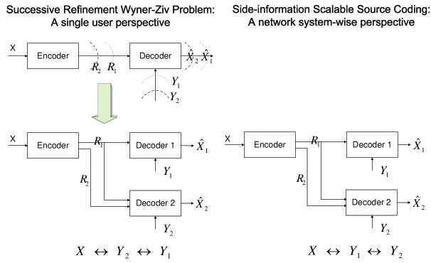
Figure 1: The SR-WZ system vs. the SI-scalable system.

Both the SR-WZ [5][6] and SI-scalable problems can be thought as special cases of the problem of scalable source coding with no specific structure imposed on the decoder SI; this general problem appears to be quite difficult, since even without the scalable requirement, a complete solution to the problem has not been found [7]. Here we emphasize that the SR-WZ and the SI-scalable problem are quite different in terms of their applications, though they seem similar since only the order of SI quality that is reversed. Roughly speaking, in the SI-scalable problem, the side information $Y_{2}$ at the later stage is worse than the side information $Y_{1}$ at the early stage, while in the SR-WZ problem, the order is reversed. In more mathematically precise terms, for the SI-scalable problem, the side informations are degraded as $X\leftrightarrow Y_{1}\leftrightarrow Y_{2}$, in contrast to the SR-WZ problem where the reversed order is specified as $X\leftrightarrow Y_{2}\leftrightarrow Y_{1}$. The two problems are also different in terms of their possible applications. The SR-WZ problem is more applicable for a single server-user pair, when the user is receiving side information through another channel, and at the same time receiving the description(s) from the server; for this scenario, two decoders can be extracted to provide a simplified model. On the other hand, the SI-scalable problem is more applicable when multiple users exist in the network, and the server wants to provide a scalable description, such that the good user is not jeopardized unnecessarily (see Fig. 1).

It is also worth pointing out that Heegard and Berger showed when the scalable coding requirement is removed, the optimal encoding by itself is in fact naturally progressive from the bad user to the good one; as such, the SI-scalable problem is expected to be more difficult than the SR-WZ problem, since the encoding order is reversed from the natural one. This difficulty is encapsulated by the fact that in the SR-WZ ordering the decoder with better SI is able to decode whatever message was meant for the decoder with worse SI and hence the first stage can be maximally useful. However, in the SI-scalable problem an additional tension exists in the sense that the second-stage decoder will need extra information to disambiguate the information of the first stage.

The problem is well understood for the lossless case. The key difference from the lossy case is that the quality of the side informations can be naturally determined by the value of $H(X|Y)$. By the seminal work of Slepian and Wolf [9], $H(X|Y)$ is the minimum rate of encoding $X$ losslessly with side information $Y$ at the decoder, thus in a sense a larger $H(X|Y)$ corresponds to weaker side information. If $H(X|Y_{1})<H(X|Y_{2})$, then the rate $(R_{1},R_{2})=(H(X|Y_{1}),H(X|Y_{2})-H(X|Y_{1}))$ is achievable, as noticed by Feder and Shulman [10]. Extending this observation and a coding scheme in [11], Draper [12] proposed a universal incremental Slepian-Wolf coding scheme when the distribution is unknown, which inspired Eckford and Yu [13] to design rateless Slepian-Wolf LDPC code. For the lossless case, there is no loss of optimality by using a scalable coding approach; an immediate question is to ask whether the same is true for the lossy case in terms of rate distortion, which we will show to be not so in general. In this rate-distortion setting, the order of goodness by the value of $H(X|Y)$ is not sufficient because of the presence of the distortion constraints. This motivates the Markov condition $X\leftrightarrow Y_{1}\leftrightarrow Y_{2}$ introduced for the SI-scalable coding problem. Going further along this point of view, the SI-scalable problem is also applicable in the single user setting, when the source encoder does not know exactly which side information the receiver has within a given set. Therefore it can be viewed as a special case of the side-information universal rate distortion coding.

In this work, we formulate the problem of side information scalable source coding, and provide two inner bounds and two outer bounds for the rate-distortion region. One of the inner-bounds has the same distortion and rate expressions as one of the outer bounds, and they differ in the domain of optimization only by a Markov string requirement. Though the inner and the outer bounds do not coincide in general, the inner bounds are indeed tight for the case when either the first stage or the second stage requires a lossless reconstruction, as well as for the case when certain deterministic distortion measures are taken. Furthermore, a conclusive result is given for the quadratic Gaussian source with any finite number of stages and arbitrary correlated Gaussian side informations.

With this set of inner and outer bounds, the problem of perfect scalability is investigated, defined as when both of the layers can achieve the corresponding Wyner-Ziv bounds; this is similar to the notion of (strict) successive refinability in the SR-WZ problem [5][6]. Necessary and sufficient conditions are derived for general discrete memoryless sources to be perfectly scalable under a mild support condition. By using the tool of rate-loss introduced by Zamir [14], we further show that the gap between the inner bounds and the outer bounds are bounded by a constant when squared error distortion measure is used, and thus the inner bounds are “nearly sufficient”, in the sense as given in [15].

In addition to the result for the Gaussian source, partial result is provided for the doubly symmetric binary source (DSBS) with Hamming distortion measure when the second stage does not have side information, for which the inner bounds and outer bounds coincide in certain distortion regimes. It is shown one of the outer bound can be strictly better than the other for this source.

The rest of the paper is organized as follows. In Section II we define the problem and establish the notation. In Section III, we provide inner and outer bounds to the rate-distortion region and show that the bounds coincide in certain special cases. The notion of perfectly scalable is introduced in Section IV together with the example of a binary source. The rate loss method is applied in Section V to show the gap between the inner bound and the outer bounds is bounded. In VI, the Gaussian source is treated within a more general setting. We conclude the paper in Section VII.

II Notation and Preliminaries

Let $\mathcal{X}$ be a finite set and let $\mathcal{X}^{n}$ be the set of all $n$-vectors with components in $\mathcal{X}$. Denote an arbitrary member of $\mathcal{X}^{n}$ as $x^{n}=(x_{1},x_{2},\ldots,x_{n})$, or alternatively as $x$. Upper case is used for random variables and vectors. A discrete memoryless source (DMS) $(\mathcal{X},P_{X})$ is an infinite sequence $\{X_{i}\}_{i=1}^{\infty}$ of independent copies of a random variable $X$ in $\mathcal{X}$ with a generic distribution $P_{X}$ with $P_{X}(x^{n})=\prod_{i=1}^{n}P_{X}(x_{i})$. Similarly, let $(\mathcal{X},\mathcal{Y}_{1},\mathcal{Y}_{2},P_{XY_{1}Y_{2}})$ be a discrete memoryless three-source with generic distribution $P_{XY_{1}Y_{2}}$; the subscript will be dropped when it is clear from the context as $P(X,Y_{1},Y_{2})$.

Let $\hat{\mathcal{X}}_{1}$ and $\hat{\mathcal{X}}_{2}$ be finite reconstruction alphabets. Let $\mathit{d}_{j}:\mathcal{X}\times\hat{\mathcal{X}}_{j}\rightarrow\left[0,\infty\right)$, $j=1,2$ be two distortion measures. The single-letter distortion extension of $d_{j}$ to vectors is defined as

$$\mathit{d}_{j}(\mbox{\boldmath$x$},\mbox{\boldmath$\hat{x}$})=\frac{1}{n}\sum_{i=1}^{n}\mathit{d}_{j}(x_{i},\hat{x}_{i}),\quad\forall\mbox{\boldmath$x$}\in\mathcal{X}^{n},\quad\mbox{\boldmath$\hat{x}$}\in\hat{\mathcal{X}}_{j}^{n},\quad\quad j=1,2.$$ (1)

Definition 1

An $(n,M_{1},M_{2},D_{1},D_{2})$ rate distortion (RD) SI-scalable code for source $X$ with side information $(Y_{1},Y_{2})$ consists of two encoding functions $\phi_{i}$ and two decoding functions $\psi_{i}$, $i=1,2$:

$$\phi_{1}:\mathcal{X}^{n}\rightarrow I_{M_{1}}, \phi_{2}:\mathcal{X}^{n}\rightarrow I_{M_{2}},$$ (2)

$$\psi_{1}:I_{M_{1}}\times\mathcal{Y}_{1}^{n}\rightarrow\hat{\mathcal{X}}_{1}^{n}, \psi_{2}:I_{M_{1}}\times I_{M_{2}}\times\mathcal{Y}_{2}^{n}\rightarrow\hat{\mathcal{X}}_{2}^{n},$$ (3)

where $I_{k}=\{1,2,\ldots,k\}$, such that

$$\mbox{${\mathbb{E}}$}\mathit{d}_{1}(X^{n},\psi_{1}(\phi_{1}(X^{n}),Y_{1}^{n}))\leq D_{1},$$ (4)

$$\mbox{${\mathbb{E}}$}\mathit{d}_{2}(X^{n},\psi_{2}(\phi_{1}(X^{n}),\phi_{2}(X^{n}),Y_{2}^{n}))\leq D_{2},$$ (5)

where ${\mathbb{E}}$ is the expectation operation.

Definition 2

A rate pair $(R_{1},R_{2})$ is said to be $(D_{1},D_{2})$-achievable for SI-scalable encoding with side information $(Y_{1},Y_{2})$, if for any $\epsilon>0$ and sufficiently large $n$, there exist an $(n,M_{1},M_{2},D_{1}+\epsilon,D_{2}+\epsilon)$ RD SI-scalable code, such that $R_{1}+\epsilon\geq\frac{1}{n}\log(M_{1})$ and $R_{2}+\epsilon\geq\frac{1}{n}\log(M_{2})$.

Denote the collection of all the $(D_{1},D_{2})$-achievable rate pair $(R_{1},R_{2})$ for SI-scalable encoding as $\mathcal{R}(D_{1},D_{2})$, and we seek to characterize this region when $X\leftrightarrow Y_{1}\leftrightarrow Y_{2}$ forms a Markov string (see similar but different degradedness conditions in [5, 6]). The Markov condition in effect specifies the goodness of the side informations.

The rate-distortion function for degraded side-informations was established in [7] for the non-scalable coding problem. In light of the discussion in Section I, it gives a lower bound on the sum-rate for any RD SI-scalable code. More precisely, in order to achieve distortion $D_{1}$ with side information $Y_{1}$, and achieve distortion $D_{2}$ with side information $Y_{2}$, when $X\leftrightarrow Y_{1}\leftrightarrow Y_{2}$, the rate-distortion function is

$$R_{HB}(D_{1},D_{2})=\min_{p(D_{1},D_{2})}[I(X;W_{2}|Y_{2})+I(X;W_{1}|W_{2},Y_{1})],$$ (6)

where $p(D_{1},D_{2})$ is the set of all random variable $(W_{1},W_{2})\in\mathcal{W}_{1}\times\mathcal{W}_{2}$ jointly distributed with the generic random variables $(X,Y_{1},Y_{2})$, such that the following conditions are satisfied: (i) $(W_{1},W_{2})\leftrightarrow X\leftrightarrow Y_{1}\leftrightarrow Y_{2}$ is a Markov string; (ii) $\hat{X}_{1}=f_{1}(W_{1},Y_{1})$ and $\hat{X}_{2}=f_{2}(W_{2},Y_{2})$ satisfy the distortion constraints. Notice that the rate distortion function $R(D_{1},D_{2})$ given above suggests an encoding and decoding order from the bad user to the good user.

Wyner and Ziv [4] showed that under the following quite general assumption that the distortion measure is chosen in the set $\Gamma_{d}$ defined as

$$\Gamma_{d}\stackrel{{\scriptstyle\Delta}}{{=}}\{\mathit{d}(\cdot,\cdot):\mathit{d}(x,x)=0,\mbox{and }\mathit{d}(x,\hat{x})>0\mbox{ if }\hat{x}\neq x\},$$ (7)

then the rate distortion function satisfies $R_{X|Y}^{*}(0)=H(X|Y)$, where $R_{X|Y}^{*}(D)$ is the well-known Wyner-Ziv rate distortion function with side information $Y$. If the same assumption is made on the distortion measure $d_{1}(\cdot,\cdot)\in\Gamma_{d}$, then we can easily show (using an argument similar to the remark (3) in [4]) that

$$R_{HB}(0,D_{2})=\min_{p(D_{2})}[I(X;W_{2}|Y_{2})+H(X|W_{2},Y_{1})],$$ (8)

where $p(D_{2})$ is the set of all random variable $W_{2}$ such that $W_{2}\leftrightarrow X\leftrightarrow Y_{1}\leftrightarrow Y_{2}$ is a Markov string, and $\hat{X}_{2}=f_{2}(W_{2},Y_{2})$ satisfies the distortion constraint.

III Inner and Outer Bounds

To provide intuition into the the SI-scalable problem, we first examine a simple Gaussian source under the mean squared error (MSE) distortion measure, and describe the coding schemes informally.

Let $X\sim\mathcal{N}(0,\sigma_{x}^{2})$ and $Y_{1}=Y=X+N$, where $N\sim\mathcal{N}(0,\sigma_{N}^{2})$ is independent of $X$; $Y_{2}$ is simply a constant, i.e., no side information at the second decoder. $X\leftrightarrow Y_{1}\leftrightarrow Y_{2}$ is indeed a Markov string. To avoid lengthy discussion on degenerate regimes, assume $\sigma_{N}^{2}\approx\sigma_{x}^{2}$, and consider only the following extreme cases.

• $\sigma_{x}^{2}\gg D_{1}\gg D_{2}$: It is known binning with a Gaussian codebook, generated using a single-letter mechanism (i.e., as an i.i.d. product distribution of the single-letter form) as $W_{1}=X+Z_{1}$, where $Z_{1}$ is a zero-mean Gaussian random variable independent of $X$ such that $D_{1}=\mbox{${\mathbb{E}}$}[X-\mbox{${\mathbb{E}}$}(X|Y,W_{1})]^{2}$, is optimal for Wyner-Ziv coding. This coding scheme can still be used for the first stage. In the second stage, by direct enumeration in the list of possible codewords in the particular bin specified in the first stage, the exact codeword can be recovered by decoder two, who does not have any side information. Since $\sigma_{x}^{2}\gg D_{1}\gg D_{2}$, $W_{1}$ alone is not sufficient to guarantee a distortion $D_{2}$, i.e., $D_{2}\ll\mbox{${\mathbb{E}}$}[X-\mbox{${\mathbb{E}}$}(X|W_{1})]^{2}$. Thus a successive refinement codebook, say using a Gaussian random variable $W_{2}$ conditioned on $W_{1}$ such that $D_{2}=\mbox{${\mathbb{E}}$}[X-\mbox{${\mathbb{E}}$}(X|W_{1},W_{2})]^{2}$, is needed. This leads to the achievable rates:

  $$R_{1}\geq I(X;W_{1}|Y),\quad R_{1}+R_{2}\geq I(X;W_{1}|Y)+I(W_{1};Y)+I(X;W_{2}|W_{1})=I(X;W_{1},W_{2}).$$ (9)

• $\sigma_{x}^{2}\gg D_{2}\gg D_{1}$: If we choose $W_{1}=X+Z_{1}$ such that $D_{1}=\mbox{${\mathbb{E}}$}[X-\mbox{${\mathbb{E}}$}(X|Y,W_{1})]^{2}$ and use the coding method in the previous case, then since $D_{2}\gg D_{1}$, $W_{1}$ is sufficient to achieve distortion $D_{2}$, i.e., $D_{2}\gg\mbox{${\mathbb{E}}$}[X-\mbox{${\mathbb{E}}$}(X|W_{1})]^{2}$. The rate needed for the enumeration is $I(W_{1};Y)$, and it is rather wasteful since $W_{1}$ is more than we need. To solve this problem, we construct a coarser description using random variable $W_{2}=X+Z_{1}+Z_{2}$, such that $D_{2}=\mbox{${\mathbb{E}}$}[X-\mbox{${\mathbb{E}}$}(X|W_{2})]^{2}$. The encoding process has three effective layers for the needed two stages: (i) the first layer uses Wyner-Ziv coding with codewords generated by $P_{W_{2}}$ (ii) the second layer uses successive refinement Wyner-Ziv coding with $P_{W_{1}|W_{2}}$ (iii) the third layer enumerates the specific $W_{2}$ codeword within the first layer bin. Note that the first two layers form a SR-WZ scheme with identical side information $Y$ at the decoder. For decoding, decoder one decodes the first two layers with side information $Y$, while decoder two decodes the first and the third layer without side information. By the Markov string $X\leftrightarrow W_{1}\leftrightarrow W_{2}$, this scheme gives the following rates:

  $$R_{1} \geq I(X;W_{1},W_{2}|Y)=I(X;W_{1}|Y)$$

  $$R_{1}+R_{2} \geq I(X;W_{1}|Y)+I(W_{2};Y)=I(X;W_{2})+I(X;W_{1}|Y,W_{2}).$$ (10)

It is seen in the above discussion the specific coding schemes depend on the distortion values, which is not desirable since this usually suggests difficulty in proving the converse. The two coding schemes can be unified into a single one by introducing an auxiliary random variable, as will be shown in the sequel, however, it appears the converse is indeed quite difficult to prove.

In the rest of this section, inner and outer bounds for $\mathcal{R}(D_{1},D_{2})$ are provided. The coding schemes for the above Gaussian example are naturally generalized to give the inner bounds. It is further shown that the inner bounds are in fact tight for certain special cases.

III-A Two inner bounds

Define the region $\mathcal{R}_{in}(D_{1},D_{2})$ to be the set of all rate pairs $(R_{1},R_{2})$ for which there exist random variables $(W_{1},W_{2},V)$ in finite alphabets $\mathcal{W}_{1},\mathcal{W}_{2},\mathcal{V}$ such that the following condition are satisfied.

1. $(W_{1},W_{2},V)\leftrightarrow X\leftrightarrow Y_{1}\leftrightarrow Y_{2}$ is a Markov string.

2. There exist deterministic maps $f_{j}:\mathcal{W}_{j}\times\mathcal{Y}_{j}\rightarrow\hat{\mathcal{X}_{j}}$ such that

   $$\mbox{${\mathbb{E}}$}\mathit{d}_{j}(X,f_{j}(W_{j},Y_{j}))\leq D_{j},\quad j=1,2.$$ (11)

3. The non-negative rate pairs satisfy:

   $$R_{1}\geq I(X;V,W_{1}|Y_{1}),\quad R_{1}+R_{2}\geq I(X;V,W_{2}|Y_{2})+I(X;W_{1}|Y_{1},V).$$ (12)

4. $W_{1}\leftrightarrow(X,V)\leftrightarrow W_{2}$ is a Markov string.

5. The alphabets $\mathcal{V}$, $\mathcal{W}_{1}$ and $\mathcal{W}_{2}$ satisfy

   $$|\mathcal{V}|\leq|\mathcal{X}|+3,\quad|\mathcal{W}_{1}|\leq|\mathcal{X}|(|\mathcal{X}|+3)+1,\quad|\mathcal{W}_{2}|\leq|\mathcal{X}|(|\mathcal{X}|+3)+1.$$ (13)

The last two conditions can be removed without causing essential difference to the region $\mathcal{R}_{in}(D_{1},D_{2})$; with them removed, no specific structure is required on the joint distribution of $(X,V,W_{1},W_{2})$. To see the last two conditions indeed do not cause loss of generality, apply the support lemma [11] as follows. For an arbitrary joint distribution of $(X,V,W_{1},W_{2})$ satisfying the first three conditions, we first reduce the cardinality of $\mathcal{V}$. To preserve $P_{X}$ and the two distortions and two mutual information values, $|\mathcal{X}|+3$ letters are needed. With this reduced alphabet, observe that both the distortion and rate expressions depend only on the marginal of $(X,V,W_{1})$ and $(X,V,W_{2})$, respectively, hence requiring $W_{1}\leftrightarrow(X,V)\leftrightarrow W_{2}$ being a Markov string does not cause any loss of generality. Next to reduce the cardinality of $\mathcal{W}_{1}$, it is seen $|\mathcal{X}||\mathcal{V}|-1$ letters are needed to preserve the joint distribution of $(X,V)$, one more is needed to preserve $D_{1}$ and another is needed to preserve $I(X;W_{1}|Y_{1},V)$. Thus $|\mathcal{X}|(|\mathcal{X}|+3)+1$ letters suffice. Note that we do not need to preserve the value of $D_{2}$ and the value of the other mutual information term because of the aforementioned Markov string. A similar argument holds for $|\mathcal{W}_{2}|$.

The following theorem asserts that $\mathcal{R}_{in}(D_{1},D_{2})$ is an achievable region.

Theorem 1

For any discrete memoryless stochastic source with side informations under the Markov condition $X\leftrightarrow Y_{1}\leftrightarrow Y_{2}$,

$$\mathcal{R}(D_{1},D_{2})\supseteq\mathcal{R}_{in}(D_{1},D_{2}).$$

This theorem is proved in Appendix B, and here we outline the coding scheme for this achievable region in an intuitive manner. The encoder first encodes using a $V$ codebook with a “coarse” binning, such that decoder one is able to decode it with side information $Y_{1}$. A Wyner-Ziv successive refinement coding (with side information $Y_{1}$) is then added conditioned on the codeword $V$ also for decoder one using $W_{1}$. The encoder then enumerates the binning of $V$ up to a level such that $V$ is decodable by decoder two using the weaker side information $Y_{2}$. By doing so, decoder two is able to reduce the number of possible codewords in the (coarse) bin to a smaller number, which essentially forms a “finer” bin; with the weaker side information $Y_{2}$, the $V$ codeword is then decoded correctly with high probability. Another Wyner-Ziv successive refinement coding (with side information $Y_{2}$) is finally added conditioned on the codeword $V$ for decoder two using a random codebook of $W_{2}$.

As seen in the above argument, in order to reduce the number of possible $V$ codewords from the first stage to the second stage, the key idea is to construct a nested binning structure as illustrated in Fig. 2. Note that this is a fundamentally different from the code structure in SR-WZ, where no nested binning is needed. Each of the coarser bin contains the same number of finer bins; each finer bin holds certain number of codewords. They are constructed in such a way that given the specific coarser bin index, the first stage decoder can decode in it with the strong side information; at the second stage, additional bitstream is received by the decoder, which further specifies one of the finer bin in the coarser bin, such that the second stage decoder can decode in this finer bin using the weaker side information. If we assign each codeword to a finer bin independently, then its coarser bin index is also independent of that of the other codewords.

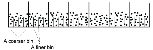
Figure 2: An illustration of the codewords in the nested binning structure.

We note that the coding scheme does not explicitly require that side informations are degraded. Indeed as long as the chosen random variable $V$ satisfies $I(V;Y_{1})\geq I(V;Y_{2})$ as well as the Markov condition, the region is indeed achievable. More precisely, the following corollary is straightforward.

Corollary 1

For any discrete memoryless stochastically source with side informations $Y_{1}$ and $Y_{2}$ (without the Markov structure), $\widetilde{\mathcal{R}}_{in}(D_{1},D_{2})\subseteq\mathcal{R}(D_{1},D_{2})$, where $\widetilde{\mathcal{R}}_{in}(D_{1},D_{2})$ is $\mathcal{R}_{in}(D_{1},D_{2})$ with the additional condition that $I(V;Y_{1})\geq I(V;Y_{2})$.

We can specialize the region $\mathcal{R}_{in}(D_{1},D_{2})$ to give another inner bound. Let $\hat{\mathcal{R}}_{in}(D_{1},D_{2})$ be the set of all rate pairs $(R_{1},R_{2})$ for which there exist random variables $(W_{1},W_{2})$ in finite alphabets $\mathcal{W}_{1},\mathcal{W}_{2}$ such that the following condition are satisfied.

1. $W_{1}\leftrightarrow W_{2}\leftrightarrow X\leftrightarrow Y_{1}\leftrightarrow Y_{2}$ or $W_{2}\leftrightarrow W_{1}\leftrightarrow X\leftrightarrow Y_{1}\leftrightarrow Y_{2}$ is a Markov string.

2. There exist deterministic maps $f_{j}:\mathcal{W}_{j}\times\mathcal{Y}_{j}\rightarrow\hat{\mathcal{X}_{j}}$ such that

   $$\mbox{${\mathbb{E}}$}\mathit{d}_{j}(X,f_{j}(W_{j},Y_{j}))\leq D_{j},\quad j=1,2.$$ (14)

3. The non-negative rate pairs satisfy:

   $$R_{1}\geq I(X;W_{1}|Y_{1}),\quad R_{1}+R_{2}\geq I(X;W_{2}|Y_{2})+I(X;W_{1}|Y_{1},W_{2}).$$ (15)

4. The alphabets $\mathcal{W}_{1}$ and $\mathcal{W}_{2}$ satisfy

   $$|\mathcal{W}_{1}|\leq(|\mathcal{X}|+3)(|\mathcal{X}|(|\mathcal{X}|+3)+1),\quad|\mathcal{W}_{1}|\leq(|\mathcal{X}|+3)(|\mathcal{X}|(|\mathcal{X}|+3)+1).$$ (16)

Corollary 2

For any discrete memoryless stochastically source with side informations under the Markov condition $X\leftrightarrow Y_{1}\leftrightarrow Y_{2}$,

$$\mathcal{R}_{in}(D_{1},D_{2})\supseteq\hat{\mathcal{R}}_{in}(D_{1},D_{2}).$$

The region $\hat{\mathcal{R}}_{in}(D_{1},D_{2})$ is particular interesting for the following reasons. Firstly, it can be explicitly matched back to the coding scheme for the simple Gaussian example. Secondly, it will be shown that one of the outer bounds has the same rate and distortion expressions as $\hat{\mathcal{R}}_{in}(D_{1},D_{2})$, only with a relaxed Markov string requirement. We now prove this corollary.

Proof of Corollary 2

When $W_{1}\leftrightarrow W_{2}\leftrightarrow X$, let $V=W_{1}$. Then the rate expressions in Theorem 1 gives

$$R_{1}\geq I(X;W_{1}|Y_{1}),\quad R_{1}+R_{2}\geq I(X;V,W_{2}|Y_{2})+I(X;W_{1}|V,Y_{1})=I(X;W_{2}|Y_{2}),$$ (17)

and therefore $\mathcal{R}_{in}(D_{1},D_{2})\supseteq\hat{\mathcal{R}}_{in}(D_{1},D_{2})$ for this case. When $W_{2}\leftrightarrow W_{1}\leftrightarrow X$, let $V=W_{2}$. Then the rate expressions in Theorem 1 gives

$$R_{1} \geq I(X;V,W_{1}|Y_{1})=I(X;W_{1}|Y_{1})$$

$$R_{1}+R_{2} \geq I(X;V,W_{2}|Y_{2})+I(X;W_{1}|V,Y_{1})=I(X;W_{2}|Y_{2})+I(X;W_{1}|W_{2},Y_{1}),$$

and therefore $\mathcal{R}_{in}(D_{1},D_{2})\supseteq\hat{\mathcal{R}}_{in}(D_{1},D_{2})$ for this case.

The cardinality bound here is larger than that in Theorem 1 because of the requirement to preserve the Markov conditions. ∎

III-B Two outer bounds

Define the following two regions, which will be shown to be two outer bounds. An obvious outer bound is given by the intersection of the Wyner-Ziv rate distortion function and the rate-distortion function for the problem considered by Heegard and Berger [7] with degraded side information $X\leftrightarrow Y_{1}\leftrightarrow Y_{2}$

$$\mathcal{R}_{\cap}(D_{1},D_{2})=\{(R_{1},R_{2}):R_{1}\geq R^{*}_{X|Y_{1}}(D_{1}),\quad R_{1}+R_{2}\geq R_{HB}(D_{1},D_{2})\}.$$ (18)

A tighter outer bound is now given as follows: define the region $\mathcal{R}_{out}(D_{1},D_{2})$ to be the set of all rate pairs $(R_{1},R_{2})$ for which there exist random variables $(W_{1},W_{2})$ in finite alphabets $\mathcal{W}_{1},\mathcal{W}_{2}$ such that the following conditions are satisfied.

1. $(W_{1},W_{2})\leftrightarrow X\leftrightarrow Y_{1}\leftrightarrow Y_{2}$.

2. There exist deterministic maps $f_{j}:\mathcal{W}_{j}\times\mathcal{Y}_{j}\rightarrow\hat{\mathcal{X}_{j}}$ such that

   $$\mbox{${\mathbb{E}}$}\mathit{d}_{j}(X,f_{j}(W_{j},Y_{j}))\leq D_{j},\quad j=1,2.$$ (19)

3. $|\mathcal{W}_{1}|\leq|\mathcal{X}|(|\mathcal{X}|+3)+2$, $|\mathcal{W}_{2}|\leq|\mathcal{X}|+3$.

4. The non-negative rate vectors satisfies:

   $$R_{1}\geq I(X;W_{1}|Y_{1}),\quad R_{1}+R_{2}\geq I(X;W_{2}|Y_{2})+I(X;W_{1}|Y_{1},W_{2}).$$ (20)

The main result of this subsection is the following theorem.

Theorem 2

For any discrete memoryless stochastically source with side informations under the Markov condition $X\leftrightarrow Y_{1}\leftrightarrow Y_{2}$,

$$\mathcal{R}_{\cap}(D_{1},D_{2})\supseteq\mathcal{R}_{out}(D_{1},D_{2})\supseteq\mathcal{R}(D_{1},D_{2}).$$

The first inclusion of $\mathcal{R}_{\cap}(D_{1},D_{2})\supseteq\mathcal{R}_{out}(D_{1},D_{2})$ is obvious, since $\mathcal{R}_{out}(D_{1},D_{2})$ takes the same form as $R^{*}_{X|Y_{1}}(D_{1})$ and $R_{HB}(D_{1},D_{2})$ when the rates $R_{1}$ and $R_{1}+R_{2}$ are considered individually. Thus we will focus on the latter inclusion, whose proof is given in Appendix C.

Note that the inner bound $\hat{\mathcal{R}}_{in}(D_{1},D_{2})$ and $\mathcal{R}_{out}(D_{1},D_{2})$ have the same rate and distortion expressions and they differ only by a Markov string requirement (ignoring the non-essential cardinality bounds). Because of the difference in the domain of optimizations, the two bounds may not produce the same rate-regions. This is quite similar to the case of distributed lossy source coding problem, for which the Berger-Tung inner bound requires a long Markov string and the Berger-Tung outer bound requires only two short Markov strings [16], but their rate and distortion expressions are the same.

III-C Lossless reconstruction at one decoder

Since decoder one has better quality side information, it is reasonable for it to require a higher quality reconstruction. Alternatively, from the point of view of universal coding, when the encoder does not know the quality of the side information, it might assume the better quality one exists at the decoder and aim to reconstruct with a higher quality, comparing with the case when the poorer quality side information is available. In the extreme case, decoder one might require a lossless reconstruction. In this subsection, we consider the setting where either decoder one or decoder two requires lossless reconstruction. We have the following theorem.

Theorem 3

If $D_{1}=0$ with $d_{1}(\cdot,\cdot)\in\Gamma_{d}$, or $D_{2}=0$ with $d_{2}(\cdot,\cdot)\in\Gamma_{d}$ (see 7 for $\Gamma_{d}$), then $\mathcal{R}(D_{1},D_{2})=\mathcal{R}_{in}(D_{1},D_{2})$. More precisely, for the former case,

$$\mathcal{R}(0,D_{2})=\bigcup_{P_{W_{2}}(D_{2})}\{(R_{1},R_{2}):R_{1}\geq H(X|Y_{1}),\quad R_{1}+R_{2}\geq I(X;W_{2}|Y_{2})+H(X|Y_{1},W_{2}).\},$$ (21)

where $P_{W_{1}}(D_{2})$ is the set of random variables satisfying the Markov string $W_{2}\leftrightarrow X\leftrightarrow Y_{1}\leftrightarrow Y_{2}$, and having a deterministic function $f_{2}$ satisfying $\mbox{${\mathbb{E}}$}d(f_{2}(W_{2},Y_{2}),X)\leq D_{2}$. For the latter case,

$$\mathcal{R}(D_{1},0)=\bigcup_{P_{W_{1}}(D_{1})}\{(R_{1},R_{2}):R_{1}\geq I(X;W_{1}|Y_{1}),\quad R_{1}+R_{2}\geq H(X|Y_{2})\},$$ (22)

where $P_{W_{1}}(D_{1})$ is the set of random variables satisfying the Markov string $W_{1}\leftrightarrow X\leftrightarrow Y_{1}\leftrightarrow Y_{2}$, and having a deterministic function $f_{1}$ satisfying $\mbox{${\mathbb{E}}$}d(f_{1}(W_{1},Y_{1}),X)\leq D_{1}$.

Proof of Theorem 3: For $D_{1}=0$, let $W_{1}=X$ and $V=W_{2}$. The achievable rate vector implied by Theorem 1 is given by

$$R_{1}\geq H(X|Y_{1}),\quad R_{1}+R_{2}\geq I(X;W_{2}|Y_{2})+H(X|Y_{1},W_{2}).$$ (23)

It is seen that this rate region is tight by the converse of Slepian-Wolf coding for rate $R_{1}$, and by (8) of Heegard-Berger coding for rate $R_{1}+R_{2}$.

For $D_{2}=0$, let $W_{1}=V$ and $W_{2}=X$. The achievable rate vector implied by Theorem 1 is given by

$$R_{1}\geq I(X;W_{1}|Y_{1}),\quad R_{1}+R_{2}\geq H(X|Y_{2}).$$ (24)

It is easily seen that this rate region is tight by the converse of Wyner-Ziv coding for rate $R_{1}$, and the converse of Slepian-Wolf coding (or more precisely, Wyner-Ziv rate distortion function $R_{X|Y_{2}}(0)$ with $d_{2}(\cdot,\cdot)\in\Gamma_{d}$ as given in [4]) for rate $R_{1}+R_{2}$. ∎

Zero distortion under a distortion measure $d\in\Gamma_{d}$ can be interpreted as lossless, however, it is a weaker requirement than that the block error probability is arbitrarily small. Nevertheless, $\mathcal{R}(0,D_{2})$ and $\mathcal{R}(D_{1},0)$ in (21) and (22) still provide valid outer bounds for the more stringent lossless definition. On the other hand, it is rather straightforward to specialize the coding scheme for these cases, and show that the same conclusion is true for lossless coding in the this case. Thus we have the following corollary.

Corollary 3

The rate region, when the first stage, and respectively the second stage, requires lossless in terms of arbitrary small block error probability is given by (21), respectively (22),

The key difference from the general case when both stages are lossy is the elimination of the need to generate one of codebooks using an auxiliary random variables, which simplifies the matter tremendously. For example when $D_{2}=0$, since the first stage encoder guarantees that $\mbox{\boldmath$w$}_{1}$ and $x$ are jointly typical, the second stage only needs to construct a codebook of $x$ by binning the approximately $2^{H(X|W_{1})}$ such $x$ vector directly. Subsequently the second stage encoder does not search for a vector $\mbox{\boldmath$x$}^{*}$ to be jointly typical with both $\mbox{\boldmath$w$}_{1}$ and $x$, but instead just sends the bin index of the observed source vector $x$ directly. Alternatively, it can be understood as both the encoder and decoder at the second stage have access to a side information vector $\mbox{\boldmath$w$}_{1}$, and thus a conditional Slepian-Wolf coding with decoder side information $Y_{2}$ suffices.

III-D Deterministic distortion measure

Another case of interest is when some functions of the source $X$ is required to be reconstructed with arbitrary small distortion in terms of Hamming distortion; see [17] for the corresponding case for the multiple description problem. More precisely, let $Q_{i}:\mathcal{X}\rightarrow\mathcal{Z}_{i}$, $i=1,2$ be two deterministic functions and denote $Z_{i}=Q_{i}(X)$. Consider the case that decoder $i$ seeks to reconstruct $Z_{i}$ with arbitrarily small Hamming distortion . The achievable region $\mathcal{R}_{in}$ is tight when the functions satisfy certain degradedness condition as stated in the following theorem.

Theorem 4

Let the distortion measure be Hamming distortion $d_{H}:\mathcal{Z}_{i}\times\mathcal{Z}_{i}\rightarrow\{0,1\}$ for $i=1,2$.

1. If there exists a deterministic function $Q^{\prime}:\mathcal{Z}_{1}\rightarrow\mathcal{Z}_{2}$ such that $Q_{2}=Q^{\prime}\cdot Q_{1}$, then $\mathcal{R}(0,0)=\mathcal{R}_{in}(0,0)$. More precisely

   $$\mathcal{R}(0,0)=\left\{(R_{1},R_{2}):R_{1}\geq H(Z_{1}|Y_{1}),\,R_{1}+R_{2}\geq H(Z_{2}|Y_{2})+H(Z_{1}|Y_{1}Z_{2})\right\}.$$ (25)

2. If there exists a deterministic function $Q^{\prime}:\mathcal{Z}_{2}\rightarrow\mathcal{Z}_{1}$ such that $Q_{1}=Q^{\prime}\cdot Q_{2}$, then $\mathcal{R}(0,0)=\mathcal{R}_{in}(0,0)$. More precisely

   $$\mathcal{R}(0,0)=\left\{(R_{1},R_{2}):R_{1}\geq H(Z_{1}|Y_{1}),\,R_{1}+R_{2}\geq H(Z_{2}|Y_{2})\right\}.$$ (26)

Proof of Theorem 4: To prove (25), first observe that by letting $W_{1}=Z_{1}$ and $V=W_{2}=Z_{2}$, $\mathcal{R}_{in}$ clearly reduces to the given expression. For the converse, we start from the outer bound $\mathcal{R}_{out}(0,0)$, which implies that $Z_{1}$ is a function of $W_{1}$ and $Y_{1}$, and $Z_{2}$ is a function of $W_{2}$ and $Y_{2}$. For the first stage rate $R_{1}$, we have the following chain of equalities

$$R_{1}\geq I(X;W_{1}|Y_{1})=I(X;W_{1}Z_{1}|Y_{1})\geq I(X;Z_{1}|Y_{1})=H(Z_{1}|Y_{1})-H(Z_{1}|X,Y_{1})=H(Z_{1}|Y_{1}).$$ (27)

For the sum rate, we have

$$R_{1}+R_{2} \geq I(X;W_{2}|Y_{2})+I(X;W_{1}|W_{2}Y_{1})$$

$$= I(X;W_{2}Z_{2}|Y_{2})+I(X;W_{1}|W_{2}Y_{1})$$

$$= I(X;Z_{2}|Y_{2})+I(X;W_{2}|Y_{2}Z_{2})+I(X;W_{1}|W_{2}Y_{1})$$

$$= H(Z_{2}|Y_{2})+I(X;W_{2}|Y_{2}Z_{2})+I(X;W_{1}|W_{2}Y_{1})$$

$$\stackrel{{\scriptstyle(a)}}{{\geq}} H(Z_{2}|Y_{2})+I(X;W_{2}|Y_{1}Y_{2}Z_{2})+I(X;W_{1}|W_{2}Y_{1})$$

$$\stackrel{{\scriptstyle(b)}}{{=}} H(Z_{2}|Y_{2})+I(X;W_{2}|Y_{1}Y_{2}Z_{2})+I(X;W_{1}|W_{2}Y_{1}Y_{2})$$

$$= H(Z_{2}|Y_{2})+I(X;W_{2}|Y_{1}Y_{2}Z_{2})+I(X;W_{1}|W_{2}Y_{1}Y_{2}Z_{2})$$

$$= H(Z_{2}|Y_{2})+I(X;W_{1}W_{2}|Y_{1}Y_{2}Z_{2})$$

$$\geq H(Z_{2}|Y_{2})+I(X;Z_{1}|Y_{1}Y_{2}Z_{2})$$

$$= H(Z_{2}|Y_{2})+H(Z_{1}|Y_{1}Y_{2}Z_{2})$$

$$\stackrel{{\scriptstyle(c)}}{{=}} H(Z_{2}|Y_{2})+H(Z_{1}|Y_{1}Z_{2}),$$

where (a) is due to the Markov string $W_{2}\leftrightarrow X\leftrightarrow(Y_{1}Y_{2})$ and $Z_{2}$ is function of $X$; (b) is due to the Markov string $(W_{1}W_{2})\leftrightarrow X\leftrightarrow Y_{1}\leftrightarrow Y_{2}$; (c) is due to the Markov string $(Z_{1},Z_{2})\leftrightarrow Y_{1}\leftrightarrow Y_{2}$.

Proof of part 2) (i.e., (26) relationship) is straightforward and is omitted. ∎

Clearly in the converse proof, the requirement that the functions $Q_{1}$ and $Q_{2}$ are degraded is not needed. Indeed this outer bound holds for any general functions, however the degradedness is needed for establishing the achievability of the region. If the coding is not necessarily scalable, then it can be seen the sum rate is indeed achievable, and the result above can be used to establish a non-trivial special result in the context of the problem treated by Heegard and Berger [7].

Corollary 4

Let the two function $Q_{1}$ and $Q_{2}$ be arbitrary, and let the distortion measure be Hamming distortion $d_{H}:\mathcal{Z}_{i}\times\mathcal{Z}_{i}\rightarrow\{0,1\}$ for $i=1,2$, then we have

$$R_{HB}(0,0)=H(Z_{2}|Y_{2})+H(Z_{1}|Y_{1}Z_{2}).$$ (28)

IV Perfect Scalability and a Binary Source

In this section we introduce the notion of perfect scalability, which is defined as when both the stages operate at the Wyner-Ziv rates. We further examine the doubly symmetric binary source and provide a partial characterization and investigate its scalability. The quadratic Gaussian source with jointly Gaussian side informations is treated in Section VI in a more general setting.

IV-A Perfect Scalability

The notion of the (strict) successive refinability defined in [5] for the SR-WZ problem with forward degradation in the side-informations (SI) can be applied to the reversely degraded case considered in this paper. This is done by introducing the notion of perfect scalability for the SI-scalable problem defined below.

Definition 3

A source $X$ is said to be perfectly scalable for distortion pair $(D_{1},D_{2})$, with side informations under the Markov string $X\leftrightarrow Y_{1}\leftrightarrow Y_{2}$, if

$$(R^{*}_{X|Y_{1}}(D_{1}),R^{*}_{X|Y_{2}}(D_{2})-R^{*}_{X|Y_{1}}(D_{1}))\in\mathcal{R}(D_{1},D_{2}).$$

Theorem 5

A source $X$ with side informations under the Markov string $X\leftrightarrow Y_{1}\leftrightarrow Y_{2}$, for which $\exists\,\,y_{1}\in\mathcal{Y}_{1}$ such that $P_{XY_{1}}(x,y_{1})>0$ for each $x\in\mathcal{X}$, is perfectly scalable for distortion pair $(D_{1},D_{2})$ if and only if there exist random variables $(W_{1},W_{2})$ and deterministic maps $f_{j}:\mathcal{W}_{j}\times\mathcal{Y}_{j}\rightarrow\hat{\mathcal{X}}_{j}$ such that the following conditions hold simultaneously:

1. $R_{X|Y_{j}}^{*}(D_{j})=I(X;W_{j}|Y_{j})$ and $\mbox{${\mathbb{E}}$}d_{j}(X,f_{j}(W_{1},Y_{j}))\leq D_{j}$, for $j=1,2$.

2. $W_{1}\leftrightarrow W_{2}\leftrightarrow X\leftrightarrow Y_{1}\leftrightarrow Y_{2}$ forms a Markov string.

3. The alphabet $\mathcal{W}_{1}$ and $\mathcal{W}_{2}$ satisfy $|\mathcal{W}_{1}|\leq|\mathcal{X}|(|\mathcal{X}|+3)+2$, and $|\mathcal{W}_{2}|\leq|\mathcal{X}|+3$.

The Markov string is the most crucial condition, and the substring $W_{1}\leftrightarrow W_{2}\leftrightarrow X$ is the same as one of the condition for successive refinability without side information [2][3]. The support condition essentially requires the existence of a worst letter $y_{1}$ in the alphabet $\mathcal{Y}_{1}$ such that it has non-zero probability mass for each $(x,y_{1})$ pair, $x\in\mathcal{X}$.

Proof of Theorem 5

The sufficiency being trivial, we only prove the necessity. Without loss of generality, assume $P_{X}(x)>0$ for all $x\in\mathcal{X}$. By Theorem 2, if $(R^{*}_{X|Y_{1}}(D_{1}),R^{*}_{X|Y_{2}}(D_{2})-R^{*}_{X|Y_{1}}(D_{1})$ is achievable for $(D_{1},D_{2})$, then using the tighter outer bound $\mathcal{R}_{out}(D_{1},D_{2})$ of Theorem 2, there exist random variable $W_{1},W_{2}$ in finite alphabet, whose sizes is bounded as $|\mathcal{W}_{1}|\leq|\mathcal{X}|(|\mathcal{X}|+3)+2$ and $|\mathcal{W}_{2}|\leq|\mathcal{X}|+3$, and functions $f_{1},f_{2}$ such that $(W_{1},W_{2})\leftrightarrow X\leftrightarrow Y_{1}\leftrightarrow Y_{2}$ is a Markov string, $\mbox{${\mathbb{E}}$}d_{j}(X,f_{j}(W_{j},Y_{j}))\leq D_{j}$ for $j=1,2$ and

$$R_{X|Y_{1}}^{*}(D_{1})\geq I(X;W_{1}|Y_{1}),\quad R_{X|Y_{2}}^{*}(D_{2})\geq I(X;W_{2}|Y_{2})+I(X;W_{1}|Y_{1},W_{2}).$$ (29)

It follows

$$R_{X|Y_{2}}^{*}(D_{2})\geq I(X;W_{2}|Y_{2})+I(X;W_{1}|Y_{1},W_{2})\geq I(X;W_{2}|Y_{2})\stackrel{{\scriptstyle(a)}}{{\geq}}R_{X|Y_{2}}^{*}(D_{2}),$$ (30)

where (a) follows the converse of rate-distortion theorem for Wyner-Ziv coding. Since the leftmost and the rightmost quantities are the same, all the inequalities must be equalities in (30), and it follows $I(X;W_{1}|Y_{1},W_{2})=0$. Similarly we have

$$R_{X|Y_{1}}^{*}(D_{1})\geq I(X;W_{1}|Y_{1})\geq R_{X|Y_{1}}^{*}(D_{1}),$$ (31)

thus (31) also holds with equality.

Notice that if $W_{1}\leftrightarrow W_{2}\leftrightarrow X$ is a Markov string, then we can use Corollary 2 to claim the sufficiency and complete the proof. However, this Markov condition is not true in general. This is where the support condition is needed.

For convenience, define the set

$$F(w_{2})=\{x\in\mathcal{X}:P(x,w_{2})>0\}.$$ (32)

By the Markov string $(W_{1},W_{2})\leftrightarrow X\leftrightarrow Y_{1}$, the joint distribution of $(w_{1},w_{2},x,y_{1})$ can be factorized as follows

$$P(w_{1},w_{2},x,y_{1})=P(x,y_{1})P(w_{2}|x)P(w_{1}|x,w_{2}).$$ (33)

Furthermore, $I(X;W_{1}|Y_{1},W_{2})=0$ implies the Markov string $X\leftrightarrow(W_{2},Y_{1})\leftrightarrow W_{1}$, and thus the joint distribution of $(w_{1},w_{2},x,y_{1})$ can also be factorized as follows

$$P(w_{1},w_{2},x,y_{1})=P(x,y_{1},w_{2})p(w_{1}|y_{1},w_{2})\stackrel{{\scriptstyle(a)}}{{=}}P(x,y_{1})P(w_{2}|x)P(w_{1}|y_{1},w_{2}),$$ (34)

where (a) follows by the Markov substring $W_{2}\leftrightarrow X\leftrightarrow Y_{1}\leftrightarrow Y_{2}$. Fix an arbitrary $(w_{1}^{*},w_{2}^{*})$ pair, by the assumption that $P(x,y_{1})>0$ for any $x\in\mathcal{X}$, we have

$$P(w_{2}^{*}|x)P(w_{1}^{*}|x,w_{2}^{*})=P(w_{2}^{*}|x)P(w_{1}^{*}|y_{1},w_{2}^{*})$$ (35)

for any $x\in\mathcal{X}$. Thus for any $x\in F(w_{2}^{*})$ (see definition in (32)) such that $P(w_{1}|x,w_{2}^{*})$ is well defined, we have

$$p(w_{1}^{*}|y_{1},w_{2}^{*})=p(w_{1}^{*}|x,w_{2}^{*})$$ (36)

and it further implies

$$p(w_{1}^{*}|w_{2}^{*})=\frac{\sum_{x}P(x,w_{1}^{*},w_{2}^{*})}{\sum_{x}P(x,w_{2}^{*})}=\frac{\sum_{x\in F(w_{2}^{*})}P(x,w_{2}^{*})P(w_{1}^{*}|y_{1},w_{2}^{*})}{\sum_{x}P(x,w_{2}^{*})}=p(w_{1}^{*}|y_{1},w_{2}^{*})=p(w_{1}^{*}|x,w_{2}^{*})$$ (37)

for any $x\in F(w_{2}^{*})$. This indeed implies $W_{1}\leftrightarrow W_{2}\leftrightarrow X$ is a Markov string, which completes the proof. ∎

IV-B The Doubly Symmetric Binary Source with Hamming Distortion Measure

Consider the following source: $X$ is a memoryless binary source $X\in\{0,1\}$ and $P(X=0)=0.5$. The first stage side information $Y$ can be taken as the output of a binary symmetric channel with input $X$, and crossover probability $p<0.5$. The second stage does not have side information. This source clearly satisfies the support condition in Theorem 5. It will be shown that for some distortion pairs, this source is perfectly scalable, while for others this is not possible. We next first provide partial results using $\hat{\mathcal{R}}_{in}$ and $\mathcal{R}_{\cap}$ previously given.

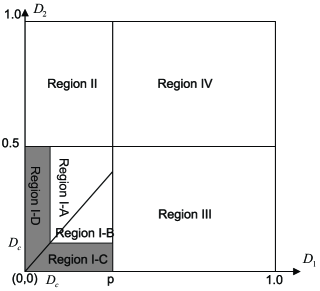
Figure 3: The partition of the distortion region, where $d_{c}$ is the critical distortion in [4] below which time sharing is not necessary.

An explicit calculation of $R_{HB}(D_{1},D_{2})$, together with the optimal forward test channel structure, was given in a recent work [6]. With this explicit calculation, it can be shown that in the shaded region in Fig. 3, the outer bound $\mathcal{R}_{\cap}(D_{1},D_{2})$ is in fact achievable (as well as in Region II, III and IV; however these three regions are degenerate cases, and will be ignored in what follows). Recall the definition of the critical distortion $d_{c}$ in the Wyner-Ziv problem for the DSBS source in [4]

$$\frac{G(d_{c})}{d_{c}-p}=G^{\prime}(d_{c}),$$

where $G(u)=h_{b}(p*u)-h_{b}(u)$, $h_{b}(u)$ is the binary entropy function $h_{b}(u)=-u\log u-(1-u)\log(1-u)$, and $u*v$ is the binary convolution for $0\leq u,v\leq 1$ as $u*v=u(1-v)+v(1-u)$. It was shown in [4] that if $D\leq d_{c}$, then $R^{*}_{X|Y}(D)=G(D)$. We will use the following result from [6].

Theorem 6

For distortion pairs $(D_{1},D_{2})$ such that $0\leq D_{2}\leq 0.5$ and $0\leq D_{1}\leq\min(d_{c},D_{2})$ (i.e., Region I-D),

$$R_{HB}(D_{1},D_{2})=1-h_{b}(D_{2}*p)+G(D_{1}).$$

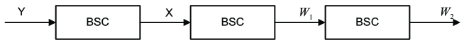
Figure 4: The forward test channel in Region I-D. The crossover probability for the BSC between $X$ and $W_{1}$ is $D_{1}$, while the crossover probability $\eta$ for the BSC between $W_{1}$ and $W_{2}$ is such that $D_{1}*\eta=D_{2}$.

This result implies that for the shaded region I-D, the forward test channel to achieve this lower bound is in fact a cascade of two BSC channels depicted in Fig. 4. This choice clearly satisfies the condition in Corollary 2 with the rates given by the outer bound $\mathcal{R}_{\cap}(D_{1},D_{2})$, which shows that this outer bound is indeed achievable. Note the following inequality

$$R_{HB}(D_{1},D_{2})=1-h_{b}(D_{2}*p)+h_{b}(p*D_{1})-h_{b}(D_{1})\geq 1-h_{b}(D_{2})=R(D_{2}),$$ (38)

where the inequality is due to the monotonicity of $G(u)$ in $0\leq u\leq 0.5$, we conclude that in this regime the source is not perfectly scalable.

To see $\mathcal{R}_{\cap}(D_{1},D_{2})$ is also achievable in region I-C, recall the result in [4] that the optimal forward test channel to achieve $R^{*}_{X|Y}(D)$ has the following structure: it is the time-sharing between zero-rate coding and a BSC with crossover probability $d_{c}$ if $D\geq d_{c}$, or a single BSC with crossover probability $D$ otherwise. Thus it is straightforward to verify that $\mathcal{R}_{\cap}(D_{1},D_{2})$ is achievable by time sharing the two forward test channels in Fig. 5; furthermore, an equivalent forward test channel can be found such that the Markov condition $W_{1}^{\prime}\leftrightarrow W_{2}\leftrightarrow X$ is satisfied, which satisfies the conditions given in Theorem 5. Thus in this regime, the source is in fact perfectly scalable.

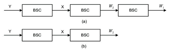
Figure 5: The forward test channels in Region I-C. The crossover probability for the BSC between $X$ and $W_{2}$ is $D_{2}$ in both the channels, while the crossover probability $\eta$ for the BSC between $W_{2}$ and $W_{1}$ in (a) is such that $D_{2}\leq D_{1}*\eta=\eta^{\prime}\leq d_{c}$. Note for (b), $W_{1}$ can be taken as a constant.

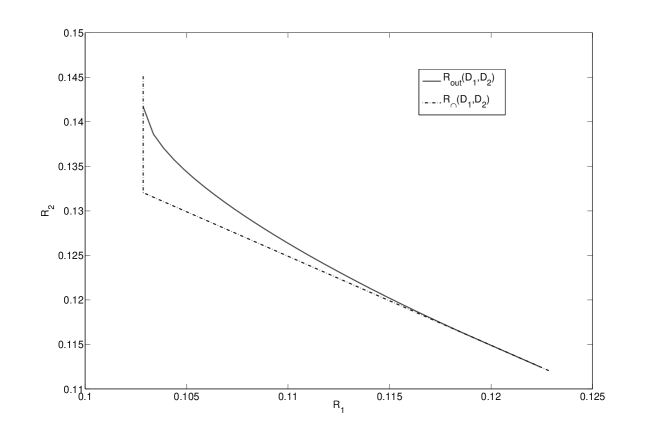
Figure 6: The rate outer bounds for a particular choice of $D_{1},D_{2}$ in Region I-B of Figure 3.

Unfortunately, we were not able to find the complete characterization for the regime I-A and I-B. Using an approach similar to [6], an explicit outer bound can be derived from $\mathcal{R}_{out}(D_{1},D_{2})$. It can then be shown numerically that for certain distortion pairs in this regime, $\mathcal{R}_{out}(D_{1},D_{2})$ is strictly tighter than $\mathcal{R}_{\cap}(D_{1},D_{2})$. This calculation can be found in [18] and is omitted here. An example is given in Fig. 6 for the two outer bounds with a non-zero gap in between for a specific distortion pair in Region I-B.

V A Near Sufficiency Result

By using the tool of rate loss introduced by Zamir [14], which was further developed in [19, 15, 20, 21], it can be shown that when both the source and reconstruction alphabets are reals, and the distortion measure is MSE, the gap between the achievable region and the out bounds are bounded by a constant. Thus the inner and outer bounds are nearly sufficient in the sense defined in [15]. To show this result, we distinguish the two cases $D_{1}\geq D_{2}$ and $D_{1}\leq D_{2}$. The source $X$ is assumed to have finite variance $\sigma_{x}^{2}$ and finite (differential) entropy. The result of this section is summarized in Fig. 7.

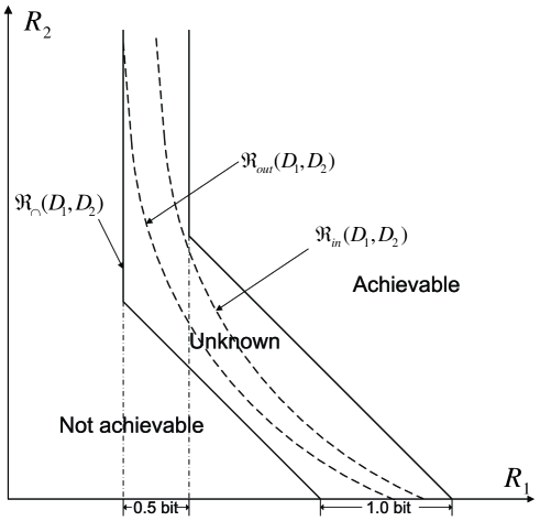
Figure 7: An illustration of the gap between the inner bound and the outer bounds when MSE is the distortion measure. The two regions $\mathcal{R}_{in}(D_{1},D_{2})$ and $\mathcal{R}_{out}(D_{1},D_{2})$ are given in dashed lines, since it is unknown whether they are indeed the same.

V-A The case $D_{1}\geq D_{2}$

Construct two random variable $W_{1}^{\prime}=X+N_{1}+N_{2}$ and $W_{2}^{\prime}=X+N_{2}$, where $N_{1}$ and $N_{2}$ are zero mean independent Gaussian random variables, independent of everything else, with variance $\sigma_{1}^{2}$ and $\sigma_{2}^{2}$ such that $\sigma_{1}^{2}+\sigma_{2}^{2}=D_{1}$ and $\sigma_{2}^{2}=D_{2}$. By letting $V^{\prime}=W^{\prime}_{1}$, it is obvious that the following rates are achievable for distortion $(D_{1},D_{2})$ from Theorem 1

$$R_{1}=I(X;X+N_{1}+N_{2}|Y_{1}),\quad R_{1}+R_{2}=I(X;X+N_{2}|Y_{2}).$$ (39)

Let $U$ be optimal random variable to achieve the Wyner-Ziv rate at distortion $D_{1}$ given decoder side information $Y_{1}$. Then it is clear that the difference between $R_{1}$ and the Wyner-Ziv rate can be bounded as,

$$I(X;X+N_{1}+N_{2}|Y_{1})-I(X;U|Y_{1})$$ (40)

$$\stackrel{{\scriptstyle(a)}}{{=}} I(X;X+N_{1}+N_{2}|UY_{1})-I(X;U|Y_{1},X+N_{1}+N_{2})$$

$$\leq I(X;X+N_{1}+N_{2}|UY_{1})$$

$$= I(X-\hat{X}_{1};X-\hat{X}_{1}+N_{1}+N_{2}|UY_{1})$$

$$\leq I(X-\hat{X}_{1},U,Y_{1};X-\hat{X}_{1}+N_{1}+N_{2})$$

$$= I(X-\hat{X}_{1};X-\hat{X}_{1}+N_{1}+N_{2})+I(U,Y_{1};X-\hat{X}_{1}+N_{1}+N_{2}|X-\hat{X}_{1})$$

$$= I(X-\hat{X}_{1};X-\hat{X}_{1}+N_{1}+N_{2})$$

$$\stackrel{{\scriptstyle(b)}}{{\leq}} \frac{1}{2}\log_{2}\frac{D_{1}+D_{1}}{D_{1}}=0.5$$

where $(a)$ is by applying chain rule to $I(X;X+N_{1}+N_{2},U|Y_{1})$ in two different ways; $(b)$ is true because $\hat{X}_{1}$ is the decoding function given $(U,Y_{1})$, the distortion between $X$ and $\hat{X}_{1}$ is bounded by $D_{1}$, and $X-\hat{X}_{1}$ is independent of $(N_{1},N_{2})$.

Now we turn to bound the gap for the sum rate $R_{1}+R_{2}$. Let $W_{1}$ and $W_{2}$ be the two random variables to achieve the rate distortion function $R_{HB}(D_{1},D_{2})$. First notice the following two identities due to the Markov string $(W_{1},W_{2})\leftrightarrow X\leftrightarrow Y_{1}\leftrightarrow Y_{2}$ and $(N_{1},N_{2})$ are independent of $(X,Y_{1},Y_{2})$

$$I(X;W_{2}|Y_{2})+I(X;W_{1}|W_{2}Y_{1}) = I(X;W_{1}W_{2}|Y_{1})+I(Y_{1};W_{2}|Y_{2})$$ (41)

$$I(X;X+N_{2}|Y_{2}) = I(X;X+N_{2}|Y_{1})+I(Y_{1};X+N_{2}|Y_{2}).$$ (42)

Next we can bound the difference between the sum-rate $R_{1}+R_{2}$ (as given in (39)) and the Heegard-Berger sum rate as follows.

$$I(X;X+N_{2}|Y_{2})-I(X;W_{2}|Y_{2})-I(X;W_{1}|W_{2}Y_{1})$$ (43)

$$= \{I(X;X+N_{2}|Y_{1})-I(X;W_{1}W_{2}|Y_{1})\}+\{I(Y_{1};X+N_{2}|Y_{2})-I(Y_{1};W_{2}|Y_{2})\}.$$

To bound the first bracket, notice that

$$I(X;X+N_{2}|Y_{1})-I(X;W_{1}W_{2}|Y_{1})$$ (44)

$$= I(X;X+N_{2}|W_{1}W_{2}Y_{1})-I(X;W_{1}W_{2}|Y_{1},X+N_{2})$$

$$\leq I(X;X+N_{2}|W_{1}W_{2}Y_{1})$$

$$\stackrel{{\scriptstyle(a)}}{{=}} I(X;X+N_{2}|W_{1}W_{2}Y_{1}Y_{2})$$

$$= I(X-\hat{X}_{2};X-\hat{X}_{2}+N_{2}|W_{1}W_{2}Y_{1}Y_{2})$$

$$\leq I(X-\hat{X}_{2},W_{1},W_{2},Y_{1},Y_{2};X-\hat{X}_{2}+N_{2})$$

$$= I(X-\hat{X}_{2};X-\hat{X}_{2}+N_{2})+I(W_{1},W_{2},Y_{1},Y_{2};X-\hat{X}_{2}+N_{2}|X-\hat{X}_{2})$$

$$= I(X-\hat{X}_{2};X-\hat{X}_{2}+N_{2})\leq\frac{1}{2}\log_{2}\frac{D_{2}+D_{2}}{D_{2}}=0.5$$

where (a) is due to the Markov string $(W_{1},W_{2})\leftrightarrow X\leftrightarrow Y_{1}\leftrightarrow Y_{2}$, $\hat{X}_{2}$ is the decoding function given $(W_{2},Y_{2})$, and the other inequalities follow similar arguments as in Eqn. (40). To bound the second bracket, we write the following

$$I(Y_{1};X+N_{2}|Y_{2})-I(Y_{1};W_{2}|Y_{2})$$ (45)

$$= I(Y_{1};X+N_{2}|W_{2}Y_{2})-I(Y_{1};W_{2}|Y_{2},X+N_{2})$$

$$\leq I(Y_{1};X+N_{2}|W_{2}Y_{2})$$

$$\leq I(XY_{1};X+N_{2}|W_{2}Y_{2})$$

$$= I(X;X+N_{2}|W_{2}Y_{2})\leq\frac{1}{2}\log_{2}\frac{D_{2}+D_{2}}{D_{2}}=0.5$$

Thus we have shown that for $D_{1}\geq D_{2}$, the gap between the outer bound $\mathcal{R}_{\cap}(D_{1},D_{2})$ and the inner bound $\mathcal{R}_{in}(D_{1},D_{2})$ is bounded. More precisely, the gap for $R_{1}$ is bounded by 0.5 bit, while the gap for the sum rate is bounded by 1.0 bit.

V-B The case $D_{1}\leq D_{2}$

Construct random variable $W_{1}^{\prime}=X+N_{1}$ and $W_{2}^{\prime}=X+N_{1}+N_{2}$, where $N_{1}$ and $N_{2}$ are zero mean independent Gaussian random variables, independent of everything else, with variance $\sigma_{1}^{2}$ and $\sigma_{2}^{2}$ such that $\sigma_{1}^{2}=D_{1}$ and $\sigma_{1}^{2}+\sigma_{2}^{2}=D_{2}$. By letting $V^{\prime}=W_{2}^{\prime}=X+N_{1}+N_{2}$, it is easily seen that the following rates are achievable for distortion $(D_{1},D_{2})$

$$R_{1} = I(X;X+N_{1}|Y_{1})$$

$$R_{1}+R_{2} = I(X;X+N_{1}+N_{2}|Y_{2})+I(X;X+N_{1}|Y_{1},X+N_{1}+N_{2}).$$

Clearly, the argument for the first stage $R_{1}$ still holds with minor changes. To bound the sum-rate gap, notice the following identity

$$I(X;X+N_{1}+N_{2}|Y_{2})+I(X;X+N_{1}|Y_{1},X+N_{1}+N_{2})$$ (46)

$$= I(X;X+N_{1}+N_{2}|Y_{1})+I(Y_{1};X+N_{1}+N_{2}|Y_{2})+I(X;X+N_{1}|Y_{1},X+N_{1}+N_{2})$$

$$= I(Y_{1};X+N_{1}+N_{2}|Y_{2})+I(X;X+N_{1}|Y_{1}).$$ (47)

Next we seek to upper bound the following quantity

$$I(X;X+N_{1}+N_{2}|Y_{2})+I(X;X+N_{1}|Y_{1},X+N_{1}+N_{2})-I(X;W_{2}|Y_{2})-I(X;W_{1}|W_{2}Y_{1})$$

$$=\{I(X;X+N_{1}|Y_{1})-I(X;W_{1}W_{2}|Y_{1})\}+\{I(Y_{1};X+N_{1}+N_{2}|Y_{2})-I(Y_{1};W_{2}|Y_{2})\},$$ (48)

where again $W_{1},W_{2}$ are the R-D optimal random variables for $R_{HB}(D_{1},D_{2})$. For the first bracket, we have

$$I(X;X+N_{1}|Y_{1})-I(X;W_{1}W_{2}|Y_{1})$$ (49)

$$= I(X;X+N_{1}|W_{1}W_{2}Y_{1})-I(X;W_{1}W_{2}|Y_{1},X+N_{1})$$

$$\leq I(X;X+N_{1}|W_{1}W_{2}Y_{1})$$

$$= I(X-\hat{X}_{1};X-\hat{X}_{1}+N_{2}|W_{1}W_{2}Y_{1})$$

$$\leq I(X-\hat{X}_{1},W_{1},W_{2},Y_{1};X-\hat{X}_{1}+N_{2})$$

$$= I(X-\hat{X}_{1};X-\hat{X}_{1}+N_{1})+I(W_{1},W_{2},Y_{1};X-\hat{X}_{1}+N_{1}|X-\hat{X}_{1})$$

$$= I(X-\hat{X}_{1};X-\hat{X}_{1}+N_{1})$$

$$\leq \frac{1}{2}\log\frac{D_{1}+D_{1}}{D_{1}}=0.5,$$

where $\hat{X}_{1}$ is the decoding function given $(W_{1},Y_{1})$. For the second bracket, following a similar approach as (45), we have

$$I(Y_{1};X+N_{1}+N_{2}|Y_{2})-I(Y_{1};W_{2}|Y_{2})$$

$$\leq I(X;X+N_{1}+N_{2}|W_{2}Y_{2})$$

$$\leq I(X-\hat{X}_{2},W_{2},Y_{2};X-\hat{X}_{2}+N_{1}+N_{2})$$

$$= I(X-\hat{X}_{2};X-\hat{X}_{2}+N_{1}+N_{2})\leq 0.5$$

Thus we conclude that for both cases the gap between the inner bound and the outer bound is bounded. Fig. 7 illustrates the inner bound and outer bounds, as well as the gap in between.

VI The Quadratic Gaussian Source with Jointly Gaussian Side Informations

The degraded side information assumption, either $X\leftrightarrow Y_{1}\leftrightarrow Y_{2}$ or $X\leftrightarrow Y_{2}\leftrightarrow Y_{1}$, for the quadratic jointly Gaussian case is especially interesting, since physically degradedness and stochastic degradedness [22] do not cause essential difference in terms of the rate-distortion region for the problem being considered [5]. Moreover, jointly Gaussian source-side information is always statistically degraded, these forwardly and reversely degraded cases together provide a complete solution to the jointly Gaussian case with two decoders.

In this section we in fact consider a more general setting with an arbitrary number of decoders for jointly Gaussian source and multiple side informations. Though the source and side informations can have arbitrary correlation, in light of the discussion above, we will treat only physically degraded side informations. Note that since a specific encoding order is specified, though the side informations are degraded as an unordered set, the quality of side informations may not be monotonic along the scalable coding order. Clearly the solution for the two stage case can be reduced in a straightforward manner from the general solution. Recall from Theorem 2 (see (18)) that $\mathcal{R}_{\cap}(D_{1},D_{2})$ is an outer bound derived from the intersection of the Heegard-Berger and Wyner-Ziv bounds. The generalization of the outer bound $\mathcal{R}_{\cap}(D_{1},D_{2})$ to $N$ decoders plays an important role, and therefore we take a detour in Section VI-A to start with the characterization of $R_{HB}(D_{1},D_{2},\ldots,D_{N})$ for the jointly Gaussian case.

VI-A $R_{HB}(D_{1},D_{2},\ldots,D_{N})$ for the jointly Gaussian case

Consider the following source $X\sim\mathcal{N}(0,\sigma_{x}^{2})$, and side informations $Y_{k}=X+\sum_{i=1}^{k}N_{i}$, where $N_{i}\sim\mathcal{N}(0,\sigma_{i}^{2})$ are mutually independent and independent of $X$. The result by Heegard and Berger [7] gives

$$R_{HB}(D_{1},D_{2},\ldots,D_{N})=\min_{p(D_{1},D_{2},\ldots,D_{N})}\sum_{k=1}^{N}I(X;W_{k}|Y_{k},W_{k+1},W_{k+2},\ldots,W_{N}),$$ (50)

where $p(D_{1},D_{2},\ldots,D_{N})$ is the set of all random variable with the Markov string $(W_{1},W_{2},\ldots,W_{N})\leftrightarrow X\leftrightarrow(Y_{1},Y_{2},\ldots,Y_{N})$, such that deterministic functions $f_{k}(Y_{k},W_{k},W_{k+1},\ldots,W_{N})$, $k=1,\ldots,N$ exist which satisfy the distortion constraints. In [6], the case $N=2$ was calculated explicitly, however such an explicit calculation appears quite involved for general $N$ due to the discussion of various cases when some of the distortion constraints are not tight. In the sequel we approach the problem by showing a jointly Gaussian forward test channel is optimal.

Note that if we choose to enforce only a subset of the distortion constraints, the rate for such a restriction gives a lower bound on $R_{HB}(D_{1},D_{2},\ldots,D_{N})$. By taking all the non-empty subsets of the distortion constraints, labeled by elements of $I_{N}=\{1,2,\ldots,N\}$, a total of $2^{N}-1$ lower bounds are available and clearly the maximum of them is also a lower bound. More precisely, we are interested in $\max R^{*}_{HB}(A_{D})$, where $A_{D}\subseteq I_{N}$ and $R^{*}_{HB}(A_{D})$ is defined in the sequel explicitly in terms of the distortion constraints only; note that if $i\in A_{D}$, $D_{i}$ is still the distortion constraint for the decoder with side information $Y_{i}$. We next derive one of these lower bounds using all the constraints $(D_{1},D_{2},\ldots,D_{N})$, i.e. $A_{D}=I_{N}$; a similar derivation applies to the case with any subset $A_{D}\subset I_{N}$. Using (50) we have,

$$\sum_{k=1}^{N}I(X;W_{k}|Y_{k},W_{k+1},W_{k+2},\ldots,W_{N})$$

$$= h(X|Y_{N})-h(X|Y_{1}W_{1}^{N})-h(X|Y_{N}W_{N})+h(X|Y_{N-1}W_{N})$$

$$\qquad\qquad-h(X|Y_{N-1}W_{N-1}^{N})+\ldots+h(X|Y_{1}W_{2}^{N})$$

$$\stackrel{{\scriptstyle(a)}}{{=}} h(X|Y_{N})-h(X|Y_{1}W_{1}^{N})$$

$$\qquad\qquad-[h(X|Y_{N}W_{N})-h(X|Y_{N-1}Y_{N}W_{N})]-\ldots-[h(X|Y_{2}W_{2}^{N})-h(X|Y_{1}Y_{2}W_{2}^{N})]$$

$$= h(X|Y_{N})-h(X|Y_{1}W_{1}^{N})-I(X;Y_{N-1}|Y_{N}W_{N})$$

$$\qquad\qquad-I(X;Y_{N-2}|Y_{N-1}W_{N-1}^{N})-\ldots-I(X;Y_{1}|Y_{2}W_{2}^{N})$$

$$\stackrel{{\scriptstyle(b)}}{{=}} h(X|Y_{N})-h(X|Y_{1}W_{1}^{N})$$

$$\qquad\qquad-[h(Y_{N-1}|Y_{N}W_{N})-h(Y_{N-1}|XY_{N})]-\ldots-[h(Y_{1}|Y_{2}W_{2}^{N})-h(Y_{1}|Y_{2}X)]$$

$$= h(X|Y_{N})+\sum_{k=2}^{N}h(Y_{k-1}|XY_{k})-\sum_{k=2}^{N}h(Y_{k-1}|Y_{k}W_{k}^{N})-h(X|Y_{1},W_{1}^{N}),$$

where (a) is because of the Markov string $X\leftrightarrow(Y_{k-1}W_{k}^{N})\leftrightarrow Y_{k}$, and (b) is because of the Markov string $W_{k}^{N}\leftrightarrow(XY_{k})\leftrightarrow Y_{k-1}$, both of which are consequences of $W_{k}^{N}\leftrightarrow X\leftrightarrow Y_{k-1}\leftrightarrow Y_{k}$. The first two terms depend only on the source and distribution $P_{XY_{1}\ldots Y_{N}}$, and we now seek to bound the latter two terms, for which we have

$$h(X|Y_{1}W_{1}^{N})=h(X-\mbox{${\mathbb{E}}$}(X|YW_{1}^{N})|YW_{1}^{N})\leq h(X-\mbox{${\mathbb{E}}$}(X|YW_{1}^{N}))\leq h(\mathcal{N}(0,D_{1}))=\frac{1}{2}\log(2\pi eD_{1}),$$ (51)

where the second inequality is because Gaussian distribution maximizes the entropy for a given second moment, and $\mbox{${\mathbb{E}}$}(X-\mbox{${\mathbb{E}}$}(X|YW_{1}^{N}))^{2}\leq D_{1}$ by the existence of the decoding function $f_{1}$. Next define

$$\gamma_{k}=\frac{\sum_{i=1}^{k-1}\sigma_{i}^{2}}{\sum_{i=1}^{k}\sigma_{i}^{2}},\,k=2,3,...,N.$$ (52)

and write the following

$$Y_{k-1} = X+\sum_{i=1}^{k-1}N_{i}=X+\sum_{i=1}^{k-1}N_{i}+\gamma_{k}\sum_{i=1}^{k}N_{i}-\gamma_{k}\sum_{i=1}^{k}N_{i}$$ (53)

$$= \gamma_{k}(X+\sum_{i=1}^{k}N_{i})+(1-\gamma_{k})X+[\sum_{i=1}^{k-1}N_{i}-\gamma_{k}\sum_{i=1}^{k}N_{i}]$$ (54)

$$= \gamma_{k}Y_{k}+(1-\gamma_{k})X+[\sum_{i=1}^{k-1}N_{i}-\gamma_{k}\sum_{i=1}^{k}N_{i}]$$ (55)

Notice that

$$\mbox{${\mathbb{E}}$}[Y_{k}(\sum_{i=1}^{k-1}N_{i}-\gamma_{k}\sum_{i=1}^{k}N_{i})]=\sum_{i=1}^{k-1}\sigma_{i}^{2}-\gamma_{k}\sum_{i=1}^{k}\sigma_{i}^{2}=0,$$ (56)

and $Y_{k}$ and $(\sum_{i=1}^{k-1}N_{i}-\gamma_{i}\sum_{i=1}^{k}N_{i})$ are jointly Gaussian, which implies that they are independent. Furthermore because $(\sum_{i=1}^{k-1}N_{i}-\gamma_{i}\sum_{i=1}^{k}N_{i})$ is independent of $X$, the Markov string $(Y_{1},Y_{2},\ldots Y_{N})\leftrightarrow X\leftrightarrow(W_{1},W_{2},\ldots,W_{N})$ implies that it is also independent of $(W_{1},W_{2},\ldots,W_{N})$. It follows

$$h(Y_{k-1}|Y_{k}W_{k}^{N}) = h\left(\gamma_{k}Y_{k}+(1-\gamma_{k})X+\sum_{i=1}^{k-1}N_{i}-\gamma_{k}\sum_{i=1}^{k}N_{i}|Y_{k}W_{k}^{N}\right)$$ (57)

$$= h\left((1-\gamma_{k})X+\sum_{i=1}^{k-1}N_{i}-\gamma_{k}\sum_{i=1}^{k}N_{i}|Y_{k}W_{k}^{N}\right)$$ (58)

$$= h\left((1-\gamma_{k})(X-\mbox{${\mathbb{E}}$}(X|Y_{k}W_{k}^{N}))+\sum_{i=1}^{k-1}N_{i}-\gamma_{k}\sum_{i=1}^{k}N_{i}|Y_{k}W_{k}^{N}\right)$$ (59)

$$\leq h\left((1-\gamma_{k})(X-\mbox{${\mathbb{E}}$}(X|Y_{k}W_{k}^{N}))+\sum_{i=1}^{k-1}N_{i}-\gamma_{k}\sum_{i=1}^{k}N_{i}\right).$$ (60)

By the aforementioned independence relation, the variance of term in the bracket is bounded above by

$$\hat{D}_{k}\stackrel{{\scriptstyle\Delta}}{{=}}(1-\gamma_{k})^{2}D_{k}+(1-\gamma_{k})^{2}\sum_{i=1}^{k-1}\sigma_{i}^{2}+\gamma_{k}^{2}\sigma_{k}^{2}.$$ (61)

Define the following quantities

$$K_{1} \stackrel{{\scriptstyle\Delta}}{{=}} h(X|Y_{N})=\frac{1}{2}\log\frac{2\pi e\sigma_{x}^{4}}{\sigma_{x}^{2}+\sum_{i=1}^{N}\sigma_{i}^{2}},$$ (62)

$$K_{k} \stackrel{{\scriptstyle\Delta}}{{=}} h(Y_{k-1}|XY_{k})=\frac{1}{2}\log\frac{2\pi e\sigma_{k}^{4}}{\sum_{i=1}^{k}\sigma_{i}^{2}},\quad k=2,3,\ldots,N$$ (63)

Summarizing the bounds in (51) and (60), we have

$$R_{HB}(D_{1},D_{2},\ldots D_{N})\geq\frac{1}{2}\log\frac{\prod_{i=1}^{N}K_{i}}{\prod_{i=1}^{N}\hat{D}_{i}}\stackrel{{\scriptstyle\Delta}}{{=}}R_{HB}^{*}(I_{N}),$$ (64)

where for convenience we define $\hat{D}_{1}=D_{1}$.

To show that $\max_{A_{D}\subseteq\{D_{1},D_{2},\ldots,D_{N}\}}R^{*}_{HB}(A_{D})$ is indeed achievable, construct the random variables $(W_{1}^{*},W_{2}^{*},\ldots,W_{N}^{*})$ as follows. Assume that $D_{k}\leq\mbox{${\mathbb{E}}$}[X-\mbox{${\mathbb{E}}$}(X|Y_{k})]^{2}$ for each $k=1,2,\ldots,N$, because otherwise this distortion requirement can be ignored completely.

[Construction of $(W_{1}^{*},W_{2}^{*},\ldots,W_{N}^{*})$]

1. For each $k=1,2,\ldots,N$, determine the variance $\sigma_{Z_{k}}^{2}$ of a Gaussian random variable $Z_{k}$ such that $D_{k}=\mbox{${\mathbb{E}}$}[X-\mbox{${\mathbb{E}}$}(X|Y_{k},X+Z_{k})]^{2}$.

2. Rank the variance of $\sigma_{Z_{k}}^{2}$ in an increasing order, and let $\omega(k)$ denote the rank of $\sigma_{Z_{k}}^{2}$.

3. Calculate $\sigma^{2}_{Z^{\prime}_{1}}=\sigma^{2}_{Z_{\omega^{-1}(1)}}$, and $\sigma^{2}_{Z^{\prime}_{k}}=\sigma^{2}_{Z_{\omega^{-1}(k)}}-\sigma^{2}_{Z_{\omega^{-1}(k-1)}}$ for $k=2,3,\ldots,N$.

4. Construct a set of independent zero-mean Gaussian random variables $(Z^{\prime}_{1},Z^{\prime}_{2},\ldots,Z^{\prime}_{N})$ to have variance $\sigma^{2}_{Z^{\prime}_{k}}$.

5. Construct a set of random variables $(W_{1}^{*},W_{2}^{*},\ldots,W_{N}^{*})$ as

   $$W_{k}^{*}=X+\sum_{i=1}^{\omega(k)}Z^{\prime}_{k}.$$ (65)

Next we show that this construction of $(W_{1}^{*},W_{2}^{*},\ldots,W_{N}^{*})$ achieves one of aforementioned lower bounds and thus is an optimal forward test channel. Choose the set $A^{*}_{D}=\{k:\omega(k)<\omega(j)\,\,\mbox{for all}\,j>k\}$, and denote the rank (in increasing order) of its element $k$ as $r(k)$. Clearly by the construction we have

$$\sum_{k=1}^{N}I(X;W^{*}_{k}|Y_{k},W^{*}_{k+1},W^{*}_{k+2},\ldots,W^{*}_{N})$$

$$= \sum_{k\in A^{*}_{D}}I(X;W^{*}_{k}|Y_{k},W^{*}_{k+1},W^{*}_{k+2},\ldots,W^{*}_{N})$$

$$= \sum_{j=1}^{|A^{*}_{D}|}I(X;W^{*}_{r^{-1}(j)}|Y_{r^{-1}(j)},W^{*}_{r^{-1}(j+1)})$$

$$= h(X|Y_{r^{-1}(|A^{*}_{D}|)})-h(X|W^{*}_{r^{-1}(|A^{*}_{D}|)}Y_{r^{-1}(|A^{*}_{D}|)})$$

$$+h(X|Y_{r^{-1}(|A^{*}_{D}|-1)}W^{*}_{r^{-1}(|A^{*}_{D}|)})-h(X|Y_{r^{-1}(|A^{*}_{D}|-1)}W^{*}_{r^{-1}(|A^{*}_{D}|-1)})$$

$$+\ldots+h(X|Y_{r^{-1}(1)}W^{*}_{r^{-1}(2})-h(X|Y_{r^{-1}(1)}W^{*}_{r^{-1}(1)})$$

$$= h(X|Y_{r^{-1}(|A^{*}_{D}|)})-h(X|Y_{r^{-1}(1)}W^{*}_{r^{-1}(1)})$$

$$-[h(Y_{r^{-1}(|A^{*}_{D}|-1)}|Y_{r^{-1}(|A^{*}_{D}|)}W^{*}_{r^{-1}(|A^{*}_{D}|)})-h(Y_{r^{-1}(|A^{*}_{D}|-1)}|XY_{r^{-1}(|A^{*}_{D}|)})]$$

$$-\ldots-[h(Y_{r^{-1}(1)}|Y_{r^{-1}(2)}W^{*}_{r^{-1}(2)})-h(Y_{r^{-1}(1)}|XY_{r^{-1}(2)})]$$

$$= R_{HB}^{*}(A^{*}_{D})$$

because of the construction of $(W_{1}^{*},W_{2}^{*},\ldots,W_{N}^{*})$ and the fact that they are jointly Gaussian with $(X,Y_{1},Y_{2},\ldots,Y_{N})$. Thus, we have proved the following theorem.

Theorem 7

The auxiliary random variable $(W_{1}^{*},W_{2}^{*},\ldots,W_{N}^{*})$ constructed above achieves the minimum in the Heegard and Berger rate distortion function for the jointly Gaussian source and side informations.

It is clear that we can determine the set $A^{*}_{D}$ before constructing $(W^{*}_{1},W^{*}_{2},\ldots,W^{*}_{N})$ using the aforementioned procedure, which can simplify the construction. However, the current construction has the advantage that each $W^{*}_{k}$ is almost individually determined by $D_{k}$, and does not substantially depend on the other distortion constraints. This will prove to be useful for the general scalable coding problem. It is worth noting that it seemingly requires comparing $2^{N}-1$ values of $R_{HB}^{*}(A_{D})$ to determine $R_{HB}(D_{1},D_{2},\ldots,D_{2})$, however, from the forward calculation we see that in fact $O(N)$ complexity suffices.

This result can be interpreted using Fig. 8. On the horizontal axis, the $N$ marks stand for the $N$ random variable $(W^{*}_{\omega^{-1}(1)},W^{*}_{\omega^{-1}(2)},\ldots,W^{*}_{\omega^{-1}(N)})$, and the on the vertical axis, the $N$ marks stand for the $N$ levels of side informations $(Y_{1},Y_{2},\ldots,Y_{N})$. The random variable pairs $(W_{k},Y_{k})$ are then the points of interest on the plane, since if the $k$-th decoder has $(Y_{k},W_{k})$ the desired distortion can be achieved; the $(W_{k},Y_{k})$ pairs are in one-to-one correspondence to the $(\omega(k),k)$ pairs. Next we associate the unit square below and to the right of each integer point $(i,j)$ is associated with a rate of value

$$R_{i,j}=I(W_{\omega^{-1}(i)};Y_{j-1}|Y_{j}W_{\omega^{-1}(i+1)})$$ (66)

where we define $W_{\omega^{-1}(N+1)}=\emptyset$, and $Y_{0}=X$. For each $k=1,2,\ldots,N$, if we cover the rectangle below and to the right of $(\omega(k),k)$, then the sum rate associated with the covered area is exactly $R_{HB}(D_{1},D_{2},\ldots,D_{N})$.

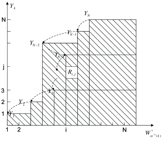
Figure 8: An illustration of the sum-rate for the Gaussian case.

With Fig. 8, the coding scheme can be understood as follows. The coding proceeds from $Y_{N}$ to $Y_{1}$, i.e., from high to low on the vertical axis; the $k$-th step ($k$-th decoder) specifies an integer point $(\omega(k),k)$, which corresponds to a $(W_{k},Y_{k})$ pair, on the figure, and additional rate is required if the area below and to the right of this point induces new area to cover. This order is illustrated in Fig. 8 along the arrows. Note that

$$\sum_{j=1}^{k}R_{i,j} = \sum_{j=1}^{k}I(W_{\omega^{-1}(i)};Y_{j-1}|Y_{j}W_{\omega^{-1}(i+1)})$$ (67)

$$= \sum_{j=1}^{k}[I(W_{\omega^{-1}(i)};Y_{j-1}|W_{\omega^{-1}(i+1)})-I(W_{\omega^{-1}(i)};Y_{j}|W_{\omega^{-1}(i+1)})]$$ (68)

$$= I(W_{\omega^{-1}(i)};X|W_{\omega^{-1}(i+1)})-I(W_{\omega^{-1}(i)};Y_{k}|W_{\omega^{-1}(i+1)})]$$ (69)

$$= I(W_{\omega^{-1}(i)};X|Y_{k}W_{\omega^{-1}(i+1)}),$$ (70)

and it is the rate for a vertical slice of hight $k$ between horizontal position $i$ and $i+1$, which is in a quite similar form as (VI-A). In this example figure, the decoders with side information $Y_{N-3}$ and $Y_{3}$ do not require additional rates. More generally, if $(\omega(k),k)$ is inside the area already covered by the previous coding steps $(N,N-1,\ldots,k+1)$, then this stage does not require additional rates. In fact, the corners of the final covered area specifies the set $A^{*}_{D}$.

The following observations are essential for the general Gaussian scalable coding problem: each unit square in Fig. 8 is not merely associated with rate $R_{i,j}$, it is in fact associated with a fraction of code $C_{i,j}$ with the following properties

1. The rate of $C_{i,j}$ is (asymptotically) $R_{i,j}$;

2. If the fractions of code associated with the area below and to the right of $(\omega(k),k)$ are available, then the decoder with side information $Y_{k}$ can decode within distortion $D_{k}$;

3. The same set of code $C_{i,j}$ can be used to fulfill only subset of the constraints, the rate calculated by the covering area method is the quadratic Gaussian Heegard and Berger rate distortion function.

The first and second observations are straightforward by constructing the nested binning together with conditional codebooks as described in Section III, i.e., $N-1$ conditioning stage from $W^{*}_{\omega^{-1}(1)}$ to $W^{*}_{\omega^{-1}(N)}$ and each conditioned codebook has $N$ nested levels from coarse for $Y_{1}$ to fine for $Y_{N}$. In fact, it is not necessary to use $N$ nested level for each codebook, but we do so for simplicity of understanding. The last property is due to the inherent Markov string among $W^{*}_{1},W^{*}_{2},\ldots,W^{*}_{N}$ and $X$.

VI-B Scalable coding with joint Gaussian side informations

Now consider the scalable coding problem where side informations and distortions are given by a permutation $\pi(\cdot)$ of that in the last subsection, i.e., $Y^{\prime}_{i}=Y_{\pi(i)}$ and $D^{\prime}_{i}=D_{\pi(i)}$. We next show that the identically permuted set of random variable $(W_{1}^{*},W_{2}^{*},\ldots,W_{N}^{*})$ achieves the Heegard-Berger rate distortion function for any first $k$ stages, thus optimal. In light of pictorial interpretation in Fig. 8, this reduces to rearranging the coded stream of $C_{i,j}$. Fig. 9 shows the effect of changing the scalable coding order.

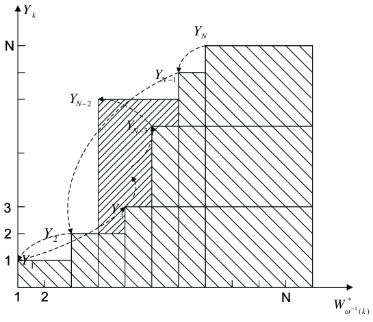
Figure 9: An illustration of incremental rate for scalable coding. The denser shaded region gives the incremental rate $R_{k}$ for the stage with side information $Y_{k}$.

More precisely, for a certain side information $Y^{\prime}_{i}=Y_{\pi(i)}$, define the following sets:

$$C(k) = \{\pi(i):i<k,\pi(i)>\pi(k)\}$$ (71)

$$E_{-}(k) = \{\pi(i):i<k,\pi(i)<\pi(k),\omega(\pi(i))>\omega(\pi(k))\},$$ (72)

and the following function

$$E(k)=\max\left[\{\pi(i):i<k,\pi(i)<\pi(k),\omega(\pi(i))<\omega(\pi(k))\}\cup\{0\}\right],$$ (73)

and let $Y_{0}=X$. Let the set of integers $E_{-}(k)$ be ordered increasingly, and the rank of its element $j$ be $r(j)$. Denote the set of random variables $\{W_{j}:j\in C\}$ as $W^{*}_{C}$ for an integer set $C$. The following $k$-th stage rate is achievable for $k=1,2,\ldots,N$

$$R_{k} = \sum_{i=1}^{|E_{-}(k)|}I(Y_{r^{-1}(i)};W^{*}_{r^{-1}(i)}|Y_{\pi(k)}W^{*}_{r^{-1}(i+1)}W^{*}_{r^{-1}(i+2)},\ldots,W^{*}_{r^{-1}(|E_{-}(k)|)}W^{*}_{C(k)})$$

$$+I(Y_{E(k)};W^{*}_{\pi(k)}|Y_{\pi(k)}W^{*}_{E_{-}(k)}W^{*}_{C(k)}).$$

It is clearly this rate corresponds to exactly the dense shaded region in Fig. 9, which is the sum of rates of fraction of codes $C(i,j)$ as described above. The property of this fraction code $C(i,j)$ thus implies the following.

Theorem 8

The Gaussian scalable coding achievable rate region for distortion vector $(D_{\pi(1)},D_{\pi(2)},\ldots,D_{\pi(N)})$ is the rate vectors $(R_{1},R_{2},\ldots,R_{N})$ satisfies

$$\sum_{i=1}^{k}R_{i}\geq R_{HB}(D_{\pi(1)},D_{\pi(2)},\ldots,D_{\pi(k)}),\quad k=1,2,...,N$$ (74)

where the side informations are $(Y_{\pi(1)},Y_{\pi(2)},\ldots,Y_{\pi(k)})$. Furthermore, it is achievable by a jointly Gaussian codebook with nested binning.

An immediate consequence of this result is the following corollary.

Corollary 5

A distortion vector $(D_{\pi(1)},D_{\pi(2)},\ldots,D_{\pi(N)})$ is perfectly scalable along side informations $(Y_{\pi(1)},Y_{\pi(2)},\ldots,Y_{\pi(k)})$ for the jointly Gaussian source if and only if $R_{HB}(D_{\pi(1)},D_{\pi(2)},\ldots,D_{\pi(k)})=R^{*}_{X|Y_{\pi(k)}}(D_{\pi(k)})$ for each $k=1,2,\ldots,N$.

This corollary applies to one of the important special cases where $D_{1}=D_{2}=\ldots=D_{N}$ and $\pi(k)=N-k+1$ for each $k$, i.e., when all the decoders have the same distortion requirement, and the scalable order is along a decreasing order of side information quality. This implies that at least for the Gaussian case, an opportunistic coding strategy does exist when the distortion requirement is the same for all the users.

VII Conclusion

We studied the problem of scalable source coding with reversely degraded side-information and gave two inner bounds as well as two outer bounds. These bounds are tight for special cases such as one lossless decoder and under certain deterministic distortion measures. Furthermore we provided a complete solution to the Gaussian source with quadratic distortion measure with any number of jointly Gaussian side informations. The problem of perfect scalability is investigated and the gap between the inner and outer bounds are shown to be bounded. For the doubly symmetric binary source with Hamming distortion, we provided partial results of the rate-distortion region. The result illustrates the difference between the lossless and the lossy source coding: though a universal approach exists with uncertain side informations at the decoder for the lossless case, such uncertainty generally causes loss of performance in the lossy case.

Appendix A Notation and Basic Properties of Typical Sequences

We will follow the definition of typicality in [11], but use a slightly different notation to make the small positive quantity $\delta$ explicit (see [5]).

Definition 4

A sequence $\mbox{\boldmath$x$}\in\mathcal{X}^{n}$ is said to be $\delta$-strongly-typical with respect to a distribution $P_{X}(x)$ on $\mathcal{X}$ if

1. For all $a\in\mathcal{X}$ with $P_{X}(a)>0$

   $$\left|\frac{1}{n}N(a|\mbox{\boldmath$x$})-P_{X}(a)\right|<\delta,$$ (75)

2. For all $a\in\mathcal{X}$ with $P_{X}(a)=0$, $N(a|\mbox{\boldmath$x$})$=0,

where $N(a|\mbox{\boldmath$x$})$ is the number of occurrences of the symbol $a$ in the sequence $x$. The set of sequences $\mbox{\boldmath$x$}\in\mathcal{X}^{n}$ that is $\delta$-strongly-typical is called the $\delta$-strongly-typical set and denoted as $T_{[X]}^{\delta}$, where the dimension $n$ is dropped.

The following properties are well-known and will be used in the proof:

1. Given a $\mbox{\boldmath$x$}\in T_{[X]}^{\delta}$, for a $y$ whose component is drawn i.i.d according to $P_{Y}$ and any $\delta^{\prime}>\delta$, we have

   $$2^{-n(I(X;Y)+\lambda_{1})}\leq P[(\mbox{\boldmath$x$},\mbox{\boldmath$y$})\in T_{[XY]}^{\delta^{\prime}}]\leq 2^{-n(I(X;Y)-\lambda_{1})}$$ (76)

   where $\lambda_{1}$ is a small positive quantity $\lambda_{1}\rightarrow 0$ as $n\rightarrow\infty$ and both $\delta,\delta^{\prime}\rightarrow 0$.

2. Similarly, given $(\mbox{\boldmath$x$},\mbox{\boldmath$y$})\in T_{[XY]}^{\delta^{\prime}}$, for any $\delta^{\prime\prime}>\delta^{\prime}$, let the component of $z$ be drawn i.i.d according to the conditional marginal $P_{Z_{i}|Y_{i}}(y_{i})$, then

   $$2^{-n(I(X;Z|Y)+\lambda_{2})}\leq P[(\mbox{\boldmath$x$},\mbox{\boldmath$y$},\mbox{\boldmath$z$})\in T_{[XYZ]}^{\delta^{\prime\prime}}]\leq 2^{-n(I(X;Z|Y)-\lambda_{2})}$$ (77)

   where $\lambda_{2}$ is a small positive quantity $\lambda_{2}\rightarrow 0$ as $n\rightarrow\infty$ and both $\delta^{\prime},\delta^{\prime\prime}\rightarrow 0$.

3. Markov Lemma [16]: If $X\leftrightarrow Y\leftrightarrow Z$ is a Markov string, and $X$ and $Y$ are such that their component is drawn independently according to $P_{XY}$. Then for all $\delta>0$

   $$\lim_{n\rightarrow\infty}P[(\mbox{\boldmath$X$},\mbox{\boldmath$z$})\in T_{[XZ]}^{|\mathcal{Y}|\delta}\left|\right(\mbox{\boldmath$Y$},\mbox{\boldmath$z$})\in T_{[YZ]}^{\delta}]\rightarrow 1.$$ (78)

   furthermore,

   $$\lim_{n\rightarrow\infty}P[(\mbox{\boldmath$X$},\mbox{\boldmath$Y$},\mbox{\boldmath$z$})\in T_{[XYZ]}^{\delta}\left|\right(\mbox{\boldmath$Y$},\mbox{\boldmath$z$})\in T_{[YZ]}^{\delta}]\rightarrow 1.$$ (79)

Appendix B Proof of Theorem 1

Codebook generation: Let a probability distribution $P_{W_{1}W_{2}XY_{1}Y_{2}}=P_{XVW_{1}W_{2}}P_{Y_{1}|X}P_{Y_{2}|Y_{1}}$, and two reconstruction functions $f_{1}(Y_{1},W_{1})$ and $f_{2}(Y_{2},W_{2})$ be given. First construct $2^{nR_{A}}$ coarser bins and $2^{nR_{A}+R_{A}^{\prime}}$ finer bins, where $R_{A}$ and $R_{A}^{\prime}$ are to be specified later. Generate $2^{R_{V}}$ length-$n$ codewords according to $P_{V}(\cdot)$, denote this set of codewords as $\mathcal{C}_{v}$; assign each of them into one of the finer bins independently. For each codeword $\mbox{\boldmath$v$}\in\mathcal{C}_{v}$, generate $2^{nR_{W_{1}}}$ length-$n$ codewords according to $P_{W_{1}|V}(\mbox{\boldmath$w_{1}$}|\mbox{\boldmath$v$})=\prod_{k=1}^{n}P_{W_{1}|V}(w_{1,k}|v_{k})$, denote this set of codewords as $\mathcal{C}_{W_{1}}(\mbox{\boldmath$v$})$; independently assign each codeword to one of the $2^{nR_{B}}$ bins. Again for each $V$ codeword, independently generate $2^{nR_{W_{2}}}$ length-$n$ codewords according to $P_{W_{2}|V}(\mbox{\boldmath$w_{2}$}|\mbox{\boldmath$v$})=\prod_{k=1}^{n}P_{W_{2}|V}(w_{2,k}|v_{k})$, denote this set of codewords as $\mathcal{C}_{W_{2}}(\mbox{\boldmath$v$})$; independently assign each codeword to one of the $2^{nR_{C}}$ bins. Reveal this codebook to the encoders and decoders.

Encoding: For a given $x$, find in $\mathcal{C}_{v}$ a codeword $\mbox{\boldmath$v$}^{*}$ such that $(\mbox{\boldmath$x$},\mbox{\boldmath$v$}^{*})\in T_{[XV]}^{2\delta}$; calculate the coarser bin index $i(\mbox{\boldmath$v$}^{*})$, and the finer bin index within the coarser bin $j(\mbox{\boldmath$v$}^{*})$. Then in the $\mathcal{C}_{w_{1}}(\mbox{\boldmath$v$}^{*})$ codebook, find a codeword $\mbox{\boldmath$w$}_{1}^{*}$ such that $(\mbox{\boldmath$w$}_{1}^{*},\mbox{\boldmath$v$}^{*},\mbox{\boldmath$x$}^{*})\in T_{[W_{1}VX]}^{3\delta}$, and calculate its corresponding bin index $k$. In $\mathcal{C}_{w_{2}}(\mbox{\boldmath$v$}^{*})$ codebook, find a codeword $\mbox{\boldmath$w$}_{2}^{*}$ such that $(\mbox{\boldmath$w$}_{2}^{*},\mbox{\boldmath$v$}^{*},\mbox{\boldmath$x$})\in T_{[W_{2}VX]}^{3\delta}$, and calculate its corresponding bin index $l$. The first-stage encoder sends $i$ and $k$, and the second-stage encoder sends $j$ and $l$. In the above procedure, if there is more than one joint-typical sequence, choose the least; if there is none, choose a default codeword and declare an error.

Decoding: The first stage decoder finds $\hat{\mbox{\boldmath$v$}}$ in the coarser bin $i$, such that $(\hat{\mbox{\boldmath$v$}},\mbox{\boldmath$y_{1}$})\in T_{[VY_{1}]}^{3|\mathcal{X}|\delta}$; then in the $\mathcal{C}_{w_{1}}(\hat{\mbox{\boldmath$v$}})$ codebook, find $\hat{\mbox{\boldmath$w_{1}$}}$ such that $(\hat{\mbox{\boldmath$w_{1}$}},\hat{\mbox{\boldmath$v$}},\mbox{\boldmath$y_{1}$})\in T_{[W_{1}VY_{1}]}^{4|\mathcal{X}|\delta}$. In the second stage, the decoder finds $\hat{\mbox{\boldmath$v$}}$ in the finer bin specified by $(i,j)$ such that $(\hat{\mbox{\boldmath$v$}},\mbox{\boldmath$y_{2}$})\in T_{[VY_{2}]}^{3|\mathcal{X}|\delta}$; then in the $\mathcal{C}_{w_{2}}(\hat{\mbox{\boldmath$v$}})$ codebook, find $\hat{\mbox{\boldmath$w_{2}$}}$ such that $(\hat{\mbox{\boldmath$w_{2}$}},\hat{\mbox{\boldmath$v$}},\mbox{\boldmath$y_{2}$})\in T_{[W_{2}VY_{2}]}^{4|\mathcal{X}|\delta}$. In the above procedure, if there is none or there are more than one, an error is declared and the decoding stops. The first decoder reconstructs as $\hat{x}_{1,k}=f_{1}(\hat{w}_{1,k},y_{1,k})$ and the second decoder as $\hat{x}_{2,k}=f_{2}(\hat{w}_{2,k},y_{2,k})$.

Probability of error: First define the encoding errors:

$$E_{0} = \{\mbox{\boldmath$X$}\notin T_{[X]}^{\delta}\}\cup\{\mbox{\boldmath$Y_{1}$}\notin T_{[Y_{1}]}^{\delta}\}\cup\{\mbox{\boldmath$Y_{2}$}\notin T_{[Y_{2}]}^{\delta}\}$$

$$E_{1} = E_{0}^{c}\cap\{\forall\mbox{\boldmath$v$}\in\mathcal{C}_{v},(\mbox{\boldmath$X$},\mbox{\boldmath$v$})\notin T_{[XV]}^{2\delta}\}$$

$$E_{2} = E_{0}^{c}\cap E_{1}^{c}\cap\{\forall\mbox{\boldmath$w_{1}$}\in\mathcal{C}_{w_{1}}(\mbox{\boldmath$v$}^{*}),(\mbox{\boldmath$w_{1}$},\mbox{\boldmath$v$}^{*},\mbox{\boldmath$X$})\notin T_{[W_{1}VX]}^{3\delta}\}$$

$$E_{3} = E_{0}^{c}\cap E_{1}^{c}\cap\{\forall\mbox{\boldmath$w_{2}$}\in\mathcal{C}_{w_{2}}(\mbox{\boldmath$v$}^{*}),(\mbox{\boldmath$w_{2}$},\mbox{\boldmath$v$}^{*},\mbox{\boldmath$X$})\notin T_{[W_{2}VX]}^{3\delta}\}.$$

Next define the decoding errors:

$$E_{4} = E_{0}^{c}\cap E_{1}^{c}\cap\{(\mbox{\boldmath$v$}^{*},\mbox{\boldmath$X$},\mbox{\boldmath$Y_{1}$})\notin T_{[VXY_{1}]}^{2\delta}\}$$

$$E_{5} = E_{0}^{c}\cap E_{1}^{c}\cap\{(\mbox{\boldmath$v$}^{*},\mbox{\boldmath$X$},\mbox{\boldmath$Y_{2}$})\notin T_{[VXY_{2}]}^{2\delta}\}$$

$$E_{6} = E_{0}^{c}\cap E_{1}^{c}\cap\{\exists\mbox{\boldmath$v$}^{\prime}\neq\mbox{\boldmath$v$}^{*}:i(\mbox{\boldmath$v$}^{\prime})=i(\mbox{\boldmath$v$}^{*})\ \text{and}\ (\mbox{\boldmath$v$}^{\prime},\mbox{\boldmath$Y_{1}$})\in T_{[VY_{1}]}^{3|\mathcal{X}|\delta}\}$$

$$E_{7} = E_{0}^{c}\cap E_{1}^{c}\cap\{\exists\mbox{\boldmath$v$}^{\prime}\neq\mbox{\boldmath$v$}^{*}:i(\mbox{\boldmath$v$}^{\prime})=i(\mbox{\boldmath$v$}^{*})\ \text{and}\ j(\mbox{\boldmath$v$}^{\prime})=j(\mbox{\boldmath$v$}^{*})\ \text{and}\ (\mbox{\boldmath$v$}^{\prime},\mbox{\boldmath$Y_{2}$})\in T_{[VY_{2}]}^{3|\mathcal{X}|\delta}\}$$

$$E_{8} = E_{0}^{c}\cap E_{1}^{c}\cap E_{2}^{c}\cap E_{4}^{c}\cap E_{6}^{c}\cap\{(\mbox{\boldmath$w^{*}_{1}$},\mbox{\boldmath$v^{*}$},\mbox{\boldmath$X$},\mbox{\boldmath$Y_{1}$})\notin T_{[W_{1}VXY_{1}]}^{3\delta}\}$$

$$E_{9} = E_{0}^{c}\cap E_{1}^{c}\cap E_{3}^{c}\cap E_{5}^{c}\cap E_{7}^{c}\cap\{(\mbox{\boldmath$w^{*}_{2}$},\mbox{\boldmath$v^{*}$},\mbox{\boldmath$X$},\mbox{\boldmath$Y_{2}$})\notin T_{[W_{2}VXY_{2}]}^{3\delta}\}$$

$$E_{10} = E_{0}^{c}\cap E_{1}^{c}\cap E_{2}^{c}\cap E_{4}^{c}\cap E_{6}^{c}\cap\{\exists\mbox{\boldmath$w^{\prime}_{1}$}\neq\mbox{\boldmath$w^{*}_{1}$}:l(\mbox{\boldmath$w^{\prime}_{1}$})=l(\mbox{\boldmath$w^{*}_{1}$})\ \text{and}\ (\mbox{\boldmath$w^{\prime}_{1}$},\mbox{\boldmath$v^{*}$},\mbox{\boldmath$Y_{1}$})\in T_{[W_{1}VY_{1}]}^{4|\mathcal{X}|\delta}\}$$

$$E_{11} = E_{0}^{c}\cap E_{1}^{c}\cap E_{3}^{c}\cap E_{5}^{c}\cap E_{7}^{c}\cap\{\exists\mbox{\boldmath$w^{\prime}_{2}$}\neq\mbox{\boldmath$w^{*}_{2}$}:l(\mbox{\boldmath$w^{\prime}_{2}$})=l(\mbox{\boldmath$w^{*}_{2}$})\ \text{and}\ (\mbox{\boldmath$w^{\prime}_{2}$},\mbox{\boldmath$v^{*}$},\mbox{\boldmath$Y_{2}$})\in T_{[W_{2}VY_{2}]}^{4|\mathcal{X}|\delta}\}$$

Apparently, for any $\epsilon^{\prime}$, for $n>n_{1}(\epsilon^{\prime},\delta)$, $P(E_{0})\leq\epsilon^{\prime}$. We have also

$$P(E_{1}) \leq P(\mbox{\boldmath$X$}\in T_{[X]}^{\delta})P(\{\forall\ \mbox{\boldmath$v$}\in\mathcal{C}_{v},\ (\mbox{\boldmath$X$},\mbox{\boldmath$v$})\notin T_{[XV]}^{2\delta}\}|\mbox{\boldmath$X$}\in T_{[X]}^{\delta})$$ (80)

$$\leq \sum_{\mbox{\boldmath$x$}\in T_{[X]}^{\delta}}P_{X}(\mbox{\boldmath$x$})(1-2^{-n(I(X;V)+\lambda)})^{nR_{1}}$$

$$\leq \exp(-2^{-n(I(X;V)+\lambda-R_{V})}),$$

where Property 1) of the typical sequences and $(1-x)^{y}<e^{-xy}$ are used. Thus $P(E_{1})\rightarrow 0$, provided that $R_{V}>I(X;V)+\lambda$.

$P(E_{4})$ and $P(E_{5})$ both tends to zero due to the Markov lemma; it requires the condition $(\mbox{\boldmath$v^{*}$},\mbox{\boldmath$X$})\in T_{[VX]}^{2\delta}$ to hold, which is indeed so given $E_{1}$ does not happen. Similarly, both $P(E_{8})$ and $P(E_{9})$ tends to zero for the same reason. Notice that if $(\mbox{\boldmath$v^{*}$},\mbox{\boldmath$X$},\mbox{\boldmath$Y_{1}$})\in T_{[VXY_{1}]}^{2\delta}$, then $(\mbox{\boldmath$v^{*}$},\mbox{\boldmath$Y_{1}$})\in T_{[VY_{1}]}^{3|\mathcal{X}|\delta}$, thus $v^{*}$ can be correctly decoded if there is no other codewords in the same bin satisfying the typicality test.

Conditioned on $E_{1}^{c}$, we have $(\mbox{\boldmath$X$},\mbox{\boldmath$v$})\in T_{[XV]}^{2\delta}$. Thus

$$P(E_{2}) \leq \sum_{(\mbox{\boldmath$x$},\mbox{\boldmath$v$})\in T_{[XV]}^{2\delta}}Pr(\mbox{\boldmath$x$},\mbox{\boldmath$v$})(1-2^{-n(I(X;W_{1}|V)+\lambda)})^{nR_{2}}$$ (81)

$$\leq \exp(-2^{-n(I(X;W_{1}|V)+\lambda_{2}-R_{2})})$$

where property 2) of the typical sequences is used. Thus $P(E_{2})$ tends to zero provided $R_{W_{1}}>I(X;W_{1}|V)+\lambda_{1}$. Similarly $P(E_{3}^{\prime})$ tends to zero provided $R_{W_{2}}>I(X;W_{2}|V)+\lambda_{2}$.

Conditioned on $E_{1}^{c}$, $\mbox{\boldmath$y_{1}$}\in T_{[Y_{1}]}^{\delta}$, since codeword in $\mathcal{C}_{v}$ are generated independently according to $P_{U}(\cdot)$

$$P(E_{6}) \leq \sum_{\mbox{\boldmath$v$}\in\mathcal{C}_{v}}2^{-nR_{A}}2^{-n(I(Y_{1};V)-\lambda_{1})}$$ (82)

$$= 2^{n(R_{V}-R_{A}-I(Y_{1};V)+\lambda_{1})}$$

where we have used property 2) of the typical sequences and the fact the bin to which $v$ is assigned is independent. Thus $P(E_{6})\rightarrow 0$ provided that $R_{A}>R_{V}-I(Y_{1};V)+\lambda_{3}$. Similarly $P(E_{7})\rightarrow 0$ provided that $R_{A}+R_{A}^{\prime}>R_{V}-I(Y_{2};V)+\lambda_{4}$.

Conditioned on $E_{4}^{c}$, $(\mbox{\boldmath$v^{*}$},\mbox{\boldmath$Y_{1}$})\in T_{[VY_{1}]}^{2|\mathcal{X}|\delta}$. Thus

$$P(E_{10}) \leq 2^{nR_{W_{1}}}2^{-nR_{B}}2^{-n(I(Y_{1};W_{1}|V)-\lambda_{3})}$$ (83)

$$= 2^{n(R_{W_{1}}-R_{B}-I(Y_{1};W_{1}|V)+\lambda_{3})}$$

where property 3) of the typical sequences is used. Thus $P(E_{10})$ tends to zero provided $R_{B}>R_{W_{1}}-I(Y_{1};W_{1}|V)+\lambda_{5}$. Similarly, $P(E_{11})$ tends to zero provided $R_{C}>R_{W_{2}}-I(Y_{2};W_{2}|V)+\lambda_{6}$. Thus the rates only need to satisfy

$$R_{1}=R_{A}+R_{B}>I(X;VW_{1}|Y_{1})+\lambda^{\prime}$$ (84)

$$R_{1}+R_{2}=R_{A}+R_{A}^{\prime}+R_{B}+R_{C}>I(X;VW_{2}|Y_{2})+I(X;W_{2}|VY_{1})+\lambda^{\prime\prime}$$ (85)

where $\lambda^{\prime}$ and $\lambda^{\prime\prime}$ are both small positive quantities and vanish as $\delta\rightarrow 0$ and $n\rightarrow\infty$; then $P_{e}\leq\sum_{i=0}^{11}P(E_{i})\rightarrow 0$. It only remains to show that the distortions constraints are satisfied as well. When no error occurs, then $(\hat{\mbox{\boldmath$W_{1}$}},\mbox{\boldmath$X$},\mbox{\boldmath$Y_{1}$})\in T_{[W_{1}XY]}^{3|\mathcal{V}|\delta}$ and $(\hat{\mbox{\boldmath$W_{2}$}},\mbox{\boldmath$X$},\mbox{\boldmath$Y_{1}$})\in T_{[W_{2}XY]}^{3|\mathcal{V}|\delta}$. By standard argument using the definition of the typical sequences, it can be shown that

$$d(\mbox{\boldmath$x$},\hat{\mbox{\boldmath$x_{1}$}})\leq\mbox{${\mathbb{E}}$}d[X,f_{1}(W_{1},Y_{1})]+\epsilon^{\prime}$$ (86)

where $\epsilon^{\prime}=\max(d(x,\hat{x}))(3|\mathcal{V}\times\mathcal{W}_{1}\times\mathcal{X}\times\mathcal{Y}_{1}|\delta+P_{e})$. Thus the distortion can be made arbitrarily small by choosing sufficiently small $\delta$ and sufficiently large $n$. Similar arguments holds for the second stage decoder. This completes the proof. ∎

Appendix C Proof of the Theorem 2

Assume the existence of $(n,M_{1},M_{2},D_{1},D_{2})$ RD SI-scalable code, there exist encoding and decoding functions $\phi_{i}$ and $\psi_{i}$ for $1=1,2$. Denote $\phi_{i}(X^{n})$ as $T_{i}$. $\mbox{\boldmath$X$}_{k}^{-}$ will be used to denote the vector $(X_{1},X_{2},\ldots,X_{k-1})$ and $\mbox{\boldmath$X$}_{k}^{+}$ to denote $(X_{k+1},X_{k+2},\ldots,X_{n})$; the subscript $k$ will be dropped when it is clear from the context. The proof follows the same line as the converse proof in [7]. The following chain of inequalities is standard (see page 440 of [22]). Here we omit the small positive quantity $\epsilon$ for simplicity.

$$nR_{1} \geq H(T_{1})\geq H(T_{1}|\mbox{\boldmath$Y_{1}$})=I(\mbox{\boldmath$X$};T_{1}|\mbox{\boldmath$Y_{1}$})=\sum_{k=1}^{n}I(X_{k};T_{1}|\mbox{\boldmath$Y_{1}$}\mbox{\boldmath$X$}_{k}^{-})$$ (87)

$$= \sum_{k=1}^{n}H(X_{k}|\mbox{\boldmath$Y_{1}$}\mbox{\boldmath$X$}_{k}^{-})-H(X_{k}|T_{1}\mbox{\boldmath$Y_{1}$}\mbox{\boldmath$X$}_{k}^{-})$$

$$= \sum_{k=1}^{n}H(X_{k}|Y_{1,k})-H(X_{k}|T_{1}\mbox{\boldmath$Y_{1}$}\mbox{\boldmath$X$}_{k}^{-})$$

$$\geq \sum_{k=1}^{n}I(X_{k};T_{1}\mbox{\boldmath$Y^{-}_{1}$}\mbox{\boldmath$Y^{+}_{1}$}|Y_{k}).$$

Next we bound the sum rate as follows

$$n(R_{1}+R_{2}) \geq H(T_{1}T_{2})\geq H(T_{1}T_{2}|\mbox{\boldmath$Y_{2}$})=I(\mbox{\boldmath$X$};T_{1}T_{2}|\mbox{\boldmath$Y_{2}$})$$

$$= I(\mbox{\boldmath$X$};T_{1}T_{2}\mbox{\boldmath$Y_{1}$}|\mbox{\boldmath$Y_{2}$})-I(\mbox{\boldmath$X$};\mbox{\boldmath$Y_{1}$}|T_{1}T_{2}\mbox{\boldmath$Y_{2}$})$$

$$= \sum_{k=1}^{n}[I(X_{k};T_{1}T_{2}\mbox{\boldmath$Y_{1}$}|\mbox{\boldmath$Y_{2}$}\mbox{\boldmath$X$}^{-})-I(\mbox{\boldmath$X$};Y_{1,k}|T_{1}T_{2}\mbox{\boldmath$Y_{2}$}\mbox{\boldmath$Y^{-}_{1}$})].$$

Since $(X_{k},Y_{2,k})$ is independent of $(\mbox{\boldmath$X$}^{-},\mbox{\boldmath$Y^{-}_{2}$},\mbox{\boldmath$Y^{+}_{2}$})$, we have

$$I(X_{k};T_{1}T_{2}\mbox{\boldmath$Y_{1}$}|\mbox{\boldmath$Y_{2}$}\mbox{\boldmath$X$}^{-})=I(X_{k};T_{1}T_{2}\mbox{\boldmath$Y_{1}$}\mbox{\boldmath$Y^{-}_{2}$}\mbox{\boldmath$Y^{+}_{2}$}\mbox{\boldmath$X$}^{-}|Y_{2,k})\geq I(X_{k};T_{1}T_{2}\mbox{\boldmath$Y_{1}$}\mbox{\boldmath$Y^{-}_{2}$}\mbox{\boldmath$Y^{+}_{2}$}|Y_{2,k})$$ (88)

The Markov condition $Y_{1,k}\leftrightarrow(X_{k},Y_{2,k})\leftrightarrow(\mbox{\boldmath$X$}^{-}\mbox{\boldmath$X$}^{+}T_{1}T_{2}\mbox{\boldmath$Y^{-}_{1}$}\mbox{\boldmath$Y^{-}_{2}$}\mbox{\boldmath$Y^{+}_{2}$})$ gives

$$I(\mbox{\boldmath$X$};Y_{1,k}|T_{1}T_{2}\mbox{\boldmath$Y_{2}$}\mbox{\boldmath$Y^{-}_{1}$})=I(X_{k};Y_{1,k}|T_{1}T_{2}\mbox{\boldmath$Y_{2}$}\mbox{\boldmath$Y^{-}_{1}$}).$$ (89)

Thus we have

$$n(R_{1}+R_{2}) \geq \sum_{k=1}^{n}[I(X_{k};T_{1}T_{2}\mbox{\boldmath$Y_{1}$}\mbox{\boldmath$Y^{-}_{2}$}\mbox{\boldmath$Y^{+}_{2}$}|Y_{2,k})-I(X_{k};Y_{1,k}|T_{1}T_{2}\mbox{\boldmath$Y_{2}$}\mbox{\boldmath$Y^{-}_{1}$})]$$ (90)

$$= \sum_{k=1}^{n}[I(X_{k};T_{1}T_{2}\mbox{\boldmath$Y^{-}_{1}$}\mbox{\boldmath$Y_{2}$}^{-}\mbox{\boldmath$Y^{+}_{2}$}|Y_{2,k})+I(X_{k};\mbox{\boldmath$Y^{+}_{1}$}|T_{1}T_{2}\mbox{\boldmath$Y_{2}$}\mbox{\boldmath$Y^{-}_{1}$}Y_{1,k})].$$

The degradedness gives $Y_{2,k}\leftrightarrow Y_{1,k}\leftrightarrow(X_{k},T_{1}T_{2},\mbox{\boldmath$Y^{-}_{1}$}\mbox{\boldmath$Y^{-}_{2}$}\mbox{\boldmath$Y^{+}_{2}$})$, which implies

$$n(R_{1}+R_{2}) \geq \sum_{k=1}^{n}[I(X_{k};T_{1}T_{2}\mbox{\boldmath$Y^{-}_{2}$}\mbox{\boldmath$Y^{+}_{2}$}\mbox{\boldmath$Y^{-}_{1}$}|Y_{2,k})+I(X_{k};\mbox{\boldmath$Y^{+}_{1}$}|T_{1}T_{2}\mbox{\boldmath$Y^{-}_{2}$}\mbox{\boldmath$Y^{+}_{2}$}\mbox{\boldmath$Y^{-}_{1}$}Y_{1,k})].$$ (91)

Define $W_{1,k}=(T_{1}\mbox{\boldmath$Y^{-}_{1}$}\mbox{\boldmath$Y^{+}_{1}$})$ and $W_{2,k}=(T_{1}T_{2}\mbox{\boldmath$Y^{-}_{2}$}\mbox{\boldmath$Y^{+}_{2}$}\mbox{\boldmath$Y^{-}_{1}$})$, by which we have

$$nR_{1} \geq \sum_{k=1}^{n}I(X_{k};W_{1,k}|Y_{1,k})$$ (92)

$$n(R_{1}+R_{2}) \geq \sum_{k=1}^{n}[I(X_{k};W_{2,k}|Y_{2,k})+I(X_{k};W_{1,k}|W_{2,k}Y_{1,k})].$$ (93)

Therefore the Markov condition $(W_{1,k},W_{2,k})\leftrightarrow X_{k}\leftrightarrow Y_{1,k}\leftrightarrow Y_{2,k}$ is true. Next introduce the time sharing random variable $Q$, which is independent of the multisource, and uniformly distributed over $I_{n}$. Define $W_{j}=(W_{j,Q},Q),\ j=1,2$. The existence of function $f_{j}$ follows by defining

$$f_{1}(W_{1},Y_{1}) = \psi_{1,Q}(\phi_{1}(\mbox{\boldmath$X$}),\mbox{\boldmath$Y_{1}$})$$ (94)

$$f_{2}(W_{2},Y_{2}) = \psi_{2,Q}(\phi_{1}(\mbox{\boldmath$X$}),\phi_{2}(\mbox{\boldmath$X$}),\mbox{\boldmath$Y_{2}$})$$ (95)

which leads the fulfillment of the distortion constraints. It only remains to show both the bound can be written in single letter form in $W_{1},W_{2}$, which is straightforward following the approach in (page 435 of) [22]. This completes the proof for $\mathcal{R}_{out}(D_{1},D_{2})\supseteq\mathcal{R}(D_{1},D_{2})$. $\blacksquare$

References

- [1] V. N. Koshelev, “Hierarchical coding of discrete sources,” Probl. Pered. Inform., vol. 16, no. 3, pp. 31–49, 1980.
- [2] W. H. R. Equitz and T. M. Cover, “Successive refinement of information,” IEEE Trans. Information Theory, vol. 37, no. 2, pp. 269–275, Mar. 1991.
- [3] B. Rimoldi, “Successive refinement of information: Characterization of achievable rates,” IEEE Trans. Information Theory, vol. 40, no. 1, pp. 253–259, Jan. 1994.
- [4] A. D. Wyner and J. Ziv, “The rate-distortion function for source coding with side information at the decoder,” IEEE Trans. Information Theory, vol. 22, no. 1, pp. 1–10, Jan. 1976.
- [5] Y. Steinberg and N. Merhav, “On successive refinement for the Wyner-Ziv problem,” IEEE Trans. Information Theory, vol. 50, no. 8, pp. 1636–1654, Aug. 2004.
- [6] C. Tian and S. Diggavi, “On multistage successive refinement for Wyner-Ziv source coding with degraded side information,” in EPFL Technical Report, Jan. 2006.
- [7] C. Heegard and T. Berger, “Rate distortion when side information may be absent,” IEEE Trans. Information Theory, vol. 31, no. 6, pp. 727–734, Nov. 1985.
- [8] A. Kaspi, “Rate-distortion when side-information may be present at the decoder,” IEEE Trans. Information Theory, vol. 40, no. 6, pp. 2031–2034, Nov. 1994.
- [9] D. Slepian and J. K. Wolf, “Noiseless coding of correlated information source,” IEEE Trans. Information Theory, vol. 19, no. 4, pp. 471–480, Jul. 1973.
- [10] M. Feder and N. Shulman, “Source broadcasting with unknown amount of receiver side information,” in Proc. IEEE Information Theory Workshop, Oct. 2002, pp. 127–130.
- [11] I. Csiszar and J. Korner, Information theory: coding theorems for discrete memoryless systems. Academic Press, New York, 1981.
- [12] S. C. Draper, “Universal incremental Slepian-Wolf coding,” in Proc. 43rd Annual Allerton Conference on communication, control and computing, Sep. 2002.
- [13] A. Eckford and W. Yu, “Rateless Slepian-Wolf codes,” in Proc. Asilomar conference on signals, systems and computers, Oct.-Nov. 2005.
- [14] R. Zamir, “The rate loss in the Wyner-Ziv problem,” IEEE Trans. Information Theory, vol. 42, no. 6, pp. 2073–2084, Nov. 1996.
- [15] L. A. Lastras and V. Castelli, “Near sufficiency of random coding for two descriptions,” IEEE Trans. Information Theory, vol. 52, no. 2, pp. 618–695, Feb. 2006.
- [16] T. Berger, “Multiterminal source coding,” in Lecture notes at CISM summer school on the information theory approach to communications, 1977.
- [17] A. E. Gamal and T. M. Cover, “Achievable rates for multiple descriptions,” IEEE Trans. Information Theory, vol. 28, no. 6, pp. 851–857, Nov. 1982.
- [18] C. Tian and S. Diggavi, “Side information scalable source coding,” in EPFL Technical Report, Sep. 2006.
- [19] L. Lastras and T. Berger, “All sources are nearly successively refinable,” IEEE Trans. Information Theory, vol. 47, no. 3, pp. 918–926, Mar. 2001.
- [20] H. Feng and M. Effros, “Improved bounds for the rate loss of multiresolution source codes,” IEEE Trans. Information Theory, vol. 49, no. 4, pp. 809–821, Apr. 2003.
- [21] H. Feng and Q. Zhao, “On the rate loss of multiresolution source codes in the Wyner-Ziv setting,” IEEE Trans. on Information Theory, vol. 52, no. 3, pp. 1164-1171, Mar. 2006.
- [22] T. M. Cover and J. A. Thomas, Elements of information theory. New York: Wiley, 1991.