LBB Stability of a Mixed Discontinuous/Continuous Galerkin Finite Element Pair

Abstract

We introduce a new mixed discontinuous/continuous Galerkin finite element for solving the 2- and 3-dimensional wave equations and equations of incompressible flow. The element, which we refer to as $\textrm{P1}_{\textrm{DG}}$-P2, uses discontinuous piecewise linear functions for velocity and continuous piecewise quadratic functions for pressure. The aim of introducing the mixed formulation is to produce a new flexible element choice for triangular and tetrahedral meshes which satisfies the LBB stability condition and hence has no spurious zero-energy modes. We illustrate this property with numerical integrations of the wave equation in two dimensions, an analysis of the resultant discrete Laplace operator in two and three dimensions, and a normal mode analysis of the semi-discrete wave equation in one dimension.

1 Introduction

One of the key strengths of the finite element method is the extensive choice of element types; this strength leads to endless discussion amongst practioners about the various benefits of different options. Alongside issues such as accuracy and practicality, a key issue is that of LBB stability. This issue manifests itself in the discretisation of the wave equation (and nonlinear extensions such as the shallow-water equations and the compressible Euler equations), and also features in the discretisation of the equations of incompressible flow. If one considers the wave equation written as a two-component system

$$\vec{u}_{t}+\nabla h=0,\quad h_{t}+\nabla\cdot\vec{u}=0,\quad\vec{u}=(u_{1},\ldots,u_{d}),$$ (1)

then finite element discretisation results in

$$\frac{\operatorname{d}}{\operatorname{d}t}M^{u}{\mathrm{u}}_{i}=-C_{i}{\mathrm{h}},\quad i=1,\ldots d,\quad\frac{\operatorname{d}}{\operatorname{d}t}M^{h}{\mathrm{h}}=\sum_{i=1}^{d}C^{T}_{i}{\mathrm{u}}_{i},$$

where $C_{i}$, $i=1,\ldots,d$ are the finite element approximations of the Cartesian components of the gradient operator, $-\sum_{i=1}^{d}C^{T}_{i}$ is the finite element approximation to the divergence operator, $M^{u}$ and $M^{h}$ are the mass matrices associated with the finite element spaces for ${\mathrm{u}}$ and ${\mathrm{h}}$ respectively, and $d$ is the number of physical dimensions. By eliminating ${\mathrm{u}}$, we obtain the discrete wave equation

$$M^{h}\frac{\operatorname{d}^{2}}{\operatorname{d}t^{2}}{\mathrm{h}}-\sum_{i}C^{T}_{i}(M^{u})^{-1}C_{i}{\mathrm{h}}=0.$$

If the discrete Laplace operator $(M^{h})^{-1}\sum_{i}C^{T}_{i}(M^{u})^{-1}C_{i}$ has null space of dimension greater than one, this results in spurious zero-energy solutions which pollute the solution after a period of time.

The null space problem also manifests itself in incompressible flow where the equations consist of a dynamical equation for $\vec{u}$ plus an incompressibility constraint which is maintained by a pressure gradient:

$$\vec{u}_{t}+N(\vec{u})=-\nabla p+\vec{F},\quad\nabla\cdot\vec{u}=0,$$

where $N$ is the advective nonlinearity and $\vec{F}$ represents all other forces. In this case the spatial discretisation becomes

$$M^{u}\frac{\operatorname{d}}{\operatorname{d}t}{\mathrm{u}}_{i}+{\mathrm{N}}_{i}({\mathrm{u}})=-C_{i}{\mathrm{p}}+{\mathrm{F}}_{i},\quad i=1,\ldots,d,\quad\sum_{i=1}^{d}C^{T}_{i}{\mathrm{u}}_{i}=0.$$

The pressure can be obtained by applying $\sum_{i}C^{T}_{i}(M^{u})^{-1}$ to the dynamical equation for $\vec{u}$ to obtain

$$0=\frac{\operatorname{d}}{\operatorname{d}t}\sum_{i}C_{i}^{T}{\mathrm{u}}_{i}=-\sum_{i}C^{T}_{i}(M^{u})^{-1}C_{i}{\mathrm{p}}-\sum_{i}C^{T}_{i}(M^{u})^{-1}({\mathrm{F}}_{i}-{\mathrm{N}}_{i}({\mathrm{u}})),\quad i=1,\ldots,d,$$

which can be solved for ${\mathrm{p}}$ (after fixing the constant component ${\mathrm{p}}_{0}$) provided that $\sum_{i}C^{T}_{i}(M^{u})^{-1}C_{i}$ has a 1-dimensional null space containing only constant functions.

The analysis of the stability properties of finite element discretisations associated with spurious eigenvectors of $\sum_{i}C^{T}_{i}(M^{u})^{-1}C_{i}$ was performed by Ladyzhenskaya [9], Babuska [2] and Brezzi [4]; as a result, a finite element discretisation is said to be LBB stable if $\sum_{i}C^{T}_{i}(M^{u})^{-1}C_{i}$ is free from spurious eigenvectors. In general these spurious eigenvectors consist of extra null vectors as well as “pesky modes” which have eigenvalues which tend to zero as the mesh size goes to zero. The spurious null vectors, which generally only occur in discretisations using structured meshes, make it impossible to invert the discrete Laplace matrix. The “pesky modes”, which arise on unstructured meshes, are nearly as problematic as they lead to very large condition numbers for the discrete Laplace matrix which make iterative methods very slow to converge. For the wave equation, a finite element discretisation is LBB stable only if the number of degrees of freedom (DOF) for $h$ is less than the number of DOF for each component of $\vec{u}$; similarly this specifies a stability condition on the number of DOF for pressure in incompressible flow. However, this is not a sufficient condition and some element choices can still be unstable despite having less DOF for $h$ than for each component of $\vec{u}$. This stability condition often leads to staggered grids (such as the $C$-grid in finite difference/volume methods) and mixed finite elements (see [7] for a discussion of mixed elements applied to the wave equation). The number of DOF for $\vec{u}$ is often increased by introducing interior modes (“bubble” functions). In this paper we suggest an alternative way of increasing the DOF for $\vec{u}$ by admitting discontinuous functions (see [8] for an review of discontinuous finite elements and their application to computational fluid dynamics, see [1, 6] for applications of discontinuous Galerkin methods to the wave equation and [11] for applications to ocean modelling), whilst keeping the continuity constraint for $h$. This often means that it is possible to increase the order of accuracy of the discretisation of $h$ whilst keeping the mixed element LBB stable. For a full treatment of LBB stability and a summary of the stability properties of a wide range of element pairs see [5]; for an analysis of element pairs applied to the linearised shallow-water equations see [13].

In section 2 we introduce the mixed discontinuous/continuous $\textrm{P1}_{\textrm{DG}}$-P2 element in one, two and three dimensions and show how the boundary conditions are implemented. We also give some values for the $h$ and $\vec{u}$ DOF which show the effects of making $\vec{u}$ discontinuous. In section 3 we compute the numerical dispersion relation for this element applied to the semi-discrete wave equation which shows that the element is indeed stable in one dimension. The numerical dispersion relation has a gap in the spectrum between two branches and we show that the modes from the lower frequency branch have smaller discontinuities in $\vec{u}$ with the lowest frequencies being nearly continuous. In section 4 we show eigenvalues of discrete Laplace matrices constructed on various unstructured grids in two and three dimensions which show that the element is stable. In section 5 we show the results of a wave equation calculation in two dimensions on an unstructured grid which illustrates the absence of spurious modes. Finally, in section 6 we give a summary of the paper and discuss other aspects of this element which may make it a good choice for ocean modelling applications.

2 The mixed element

In this section we describe our mixed element formulation in one, two and three dimensions.

2.1 Weak formulation

We start with the wave equation in the form (1) with boundary conditions

$$\frac{\partial h}{\partial n}=f\quad\mathrm{on}\quad\partial\Omega^{N},\quad h=g\quad\mathrm{on}\quad\partial\Omega^{D},$$ (2)

where $\partial\Omega^{N}$ and $\partial\Omega^{D}$ form a partition of the boundary $\partial\Omega$ of the domain $\Omega$, and multiply by test functions $\vec{w}$ and $\phi$ and integrate over the whole of $\Omega$ to obtain

$$\frac{\operatorname{d}}{\operatorname{d}t}\int_{\Omega}\vec{w}\cdot\vec{u}\operatorname{d}{V} = -\int_{\Omega}\vec{w}\cdot\nabla h\operatorname{d}{V},$$ (3)

$$\frac{\operatorname{d}}{\operatorname{d}t}\int_{\Omega}\phi h\operatorname{d}{V} = -\int_{\Omega}\phi\nabla\cdot\vec{u}\operatorname{d}{V}.$$ (4)

We then integrate equations (3)-(4) by parts, make use of the boundary conditions (2), and finally integrate equation (3) by parts again to obtain

$$\frac{\operatorname{d}}{\operatorname{d}t}\int_{\Omega}\vec{w}\cdot\vec{u}\operatorname{d}{V} = -\int_{\Omega}\vec{w}\cdot\nabla h\operatorname{d}{V}+\int_{\partial\Omega^{D}}\vec{w}\cdot\vec{n}h\operatorname{d}{S}-\int_{\partial\Omega^{D}}\vec{w}\cdot\vec{n}g\operatorname{d}{S},$$ (5)

$$\frac{\operatorname{d}}{\operatorname{d}t}\int_{\Omega}\phi h\operatorname{d}{V} = \int_{\Omega}\nabla\phi\cdot\vec{u}\operatorname{d}{V}-\int_{\partial\Omega^{D}}\vec{n}\cdot\vec{u}\phi\operatorname{d}{S}-\int_{\partial\Omega^{N}}\phi f\operatorname{d}{S},$$ (6)

which is the weak form that we discretise. The key feature of this form is that derivatives are only applied to the scalar functions $h$ and $\phi$ and not the vector functions $\vec{u}$ and $\vec{w}$ which we shall discretise with discontinuous elements.

2.2 The $\textrm{P1}_{\textrm{DG}}$-P2 element

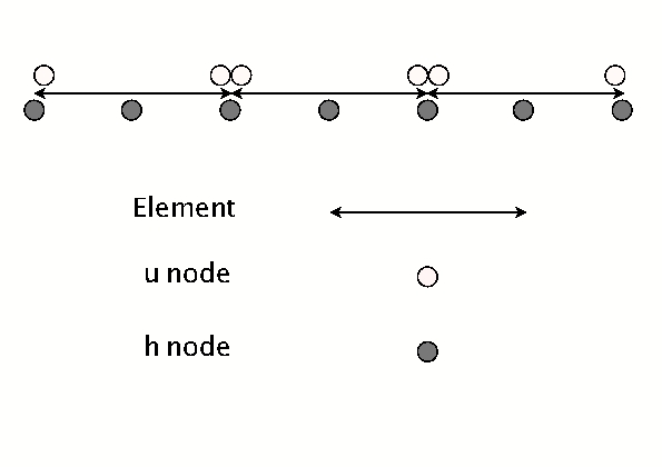
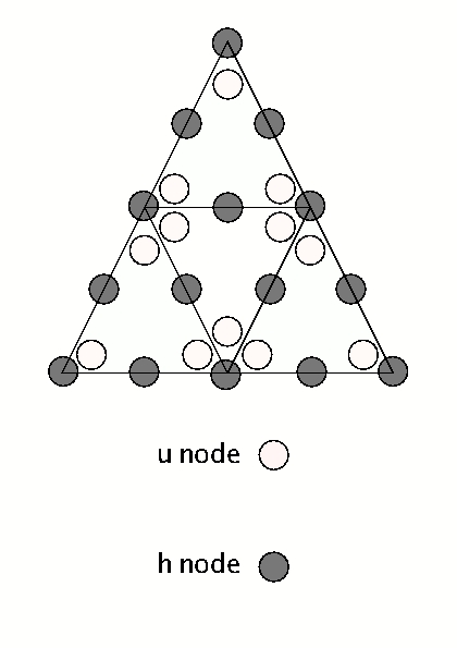
Figure 1: Figure showing the DOF for the one-dimensional $\textrm{P1}_{\textrm{DG}}$-P2 element (left) and the two-dimensional $\textrm{P1}_{\textrm{DG}}$-P2 element (right). In one dimension, each element contains two local $\vec{u}$ DOF and three local $h$ DOF, but the global $h$ DOF are constrained to be continuous across element boundaries. In two dimensions there are three local $\vec{u}$ DOF and six local $h$ DOF.

We then make the choice that the vector functions be discretised with discontinuous piecewise-linear ($\textrm{P1}_{\textrm{DG}}$) elements and the scalar functions be discretised with continuous quadratic (P2) elements. The reason for this choice is the favourable balance between $\vec{u}$ and $h$ DOF in this element.

We write the global finite element expansions in the form

$$u_{i}(\vec{x})=\sum_{\alpha=1}^{m_{u}}\mathrm{u}_{\alpha,i}N_{\alpha}(\vec{x}),\quad h(\vec{x})=\sum_{\beta=1}^{m_{h}}\mathrm{h}_{\beta}\bar{N}_{\beta}(\vec{x}),$$

where

$${\mathrm{u}}_{1,i}=[\mathrm{u}_{1,i},\ldots,\mathrm{u}_{m_{u},i}],\quad i=1,\ldots,d,\quad{\mathrm{h}}=[\mathrm{h}_{1},\ldots,\mathrm{h}_{m_{h}}],$$

and where $m_{u},m_{h}$ are the numbers of DOF for each component of $\vec{u}$ and for $h$ respectively. This leads to the following equations:

$$\frac{\operatorname{d}}{\operatorname{d}t}M^{u}{\mathrm{u}}_{i}=-C_{i}{\mathrm{h}}-{\mathrm{g}}_{i},\quad i=1,\ldots d,\quad\frac{\operatorname{d}}{\operatorname{d}t}M^{h}{\mathrm{h}}=\sum_{i=1}^{d}C^{T}_{i}{\mathrm{u}}_{i}-{\mathrm{f}},$$

where

$$M^{u}_{\alpha,\beta} = \int_{\Omega}N_{\alpha}(\vec{x})N_{\beta}(\vec{x})\operatorname{d}{V}(\vec{x}),$$

$$C_{\alpha,\beta,i} = \int_{\Omega}N_{\alpha}(\vec{x})\frac{\partial}{\partial x_{i}}\bar{N}_{\alpha}(\vec{x})\operatorname{d}{V}(\vec{x})-\int_{\partial\Omega^{D}}n_{i}N_{\alpha}(\vec{x})\bar{N}_{\beta}(\vec{x})\operatorname{d}{S},$$

$$M^{h}_{\alpha,\beta} = \int_{\Omega}\bar{N}_{\alpha}(\vec{x})\bar{N}_{\beta}(\vec{x})\operatorname{d}{V}(\vec{x}),$$

$$g_{\alpha,i} = \int_{\partial\Omega^{D}}N_{\alpha}(\vec{x})g(\vec{x})n_{i}(\vec{x})\operatorname{d}{S},$$

$$f_{\beta} = \int_{\partial\Omega^{N}}\bar{N}_{\beta}(\vec{x})f(\vec{x})\operatorname{d}{S},$$

and $d$ is the number of physical dimensions.

One of the advantages of this element choice is that the mass matrix $M^{u}$ is block diagonal (since $\vec{u}$ is discontinuous and so each global basis function is supported on only one element). This means that the discrete Laplacian $\sum_{i}C^{T}_{i}(M^{u})^{-1}C_{i}$ is still sparse and it is not necessary to lump the mass matrix when solving the pressure equation for incompressible flow.

2.2.1 One dimension

In one dimension on a bounded interval of $I$ elements, there are two local DOF per element for $u$, and so there are $2I$ global DOF as $\vec{u}$ is discontinuous. There are three local DOF per element for $h$ but there are $I-1$ global continuity constraints on the interfaces between each element (see figure 1). This means that there are $3I-(I-1)=2I+1$ global DOF for $h$, and so there is always one more $h$ DOF than $u$ DOF. However, for strong Dirichlet conditions for $h$, or periodic boundary conditions, we decrease the number of $h$ DOF and gain the potential for a stable element.

2.2.2 Two dimensions

In two dimensions we have $F$ triangular elements, with three local DOF per element $\vec{u}$ and six local DOF per element for $h$. There are no continuity constraints for $\vec{u}$ and so there are $3F$ DOF (see figure 1). There is an $h$ DOF situated at each vertex and an $h$ DOF situated on each edge, and so there are $V+E$ $h$ global DOF, where $V$ is the number of vertices and $E$ is the number of edges. Euler’s formula gives $E=V+F+1$ and so there are $2V+F+1$ $h$ DOF. This means that it is always possible to modify a mesh so that there are more $\vec{u}$ DOF than $h$ DOF e.g. by repeatedly inserting new vertices into a triangles, breaking them into four, each time increasing $V$ by 1 and $F$ by 3. In practise, useful meshes generally satisfy $F>V$ and so this property is satisfied. Strong Dirichlet boundary conditions for $\vec{u}$ may reduce the number of $\vec{u}$ DOF below that of $h$. Table 1 gives some DOF for various unstructured Delaunay meshes in a square domain.

Mesh triangles	36	79	151	1586	15574
Mesh vertices	24	48	87	820	7890
$\vec{u}$ DOF	108	237	453	4758	46722
$h$ DOF	85	176	326	2414	31354

Table 1: Table showing degrees of freedom for the $\textrm{P1}_{\textrm{DG}}$-P2 element pair in two dimensions. The ratio of $\vec{u}$ DOF to $h$ DOF appears to converge to 1.5 for large unstructured meshes.

2.2.3 Three dimensions

In three dimensions there are four local $\vec{u}$ DOF and six local $h$ DOF. As there are no continuity constraints for $\vec{u}$, there are $4T$ global $\vec{u}$ DOF, where $T$ is the total number of tetrahedra. There is one global $h$ DOF on each vertex, and one global $h$ DOF on each edge, so there are $V+E$ global $h$ DOF. As for three dimensions, it always possible to increase $T$ relative to $V+E$ by splitting elements. Table 2 gives some DOF for sample unstructured Delaunay meshes in a cubic domain.

Mesh tetrahedra	44	215	398	2003	19140
Mesh vertices	26	80	130	488	3690
Mesh edges	93	227	633	2792	24165
$\vec{u}$ DOF	176	860	1592	8012	77640
$h$ DOF	119	307	763	3280	27855

Table 2: Table showing degrees of freedom for the $\textrm{P1}_{\textrm{DG}}$-P2 element pair in three dimensions. The ratio of $\vec{u}$ DOF to $h$ DOF appears to converge to 2.5 for large unstructured meshes.

3 One-dimensional analysis

In this section we analyse the $\textrm{P1}_{\textrm{DG}}$-P2 element applied to the scalar wave equation in one-dimension on a regular grid with periodic boundary conditions.

The local (elemental) mass and gradient matrices are:

$$\bar{M}_{ij}^{u}=\int_{0}^{\Delta x}N_{i}N_{j}\operatorname{d}{x},\quad\bar{M}_{ij}^{h}=\int_{0}^{\Delta x}\bar{N}_{i}\bar{N}_{j}\operatorname{d}{x},\quad\bar{C}_{ij}=-\int_{0}^{\Delta x}N_{i}\frac{\operatorname{d}}{\operatorname{d}x}\bar{N}_{j}\operatorname{d}{x},$$

where $\{N_{1},N_{2}\}$ are the linear Lagrange polynomials used to represent $u$ in the element, $\{N_{1},N_{2},N_{3}\}$ are the quadratic Lagrange polynomials used to represent $h$, $\bar{M}^{u}$ is the local mass matrix for $u$, $\bar{M}^{h}$ is the local mass matrix for $h$ and $\bar{C}$ is the local gradient matrix. These matrices are

$$\bar{C} = \begin{pmatrix}-5/6&2/3&1/6\\ -1/6&-2/3&5/6\\ \end{pmatrix},$$

$$\bar{M}^{u} = \Delta x\begin{pmatrix}1/3&1/6\\ 1/6&1/3\\ \end{pmatrix},$$

$$\bar{M}^{h} = \Delta x\begin{pmatrix}2/15&1/15&-1/30\\ 1/15&8/15&1/15\\ -1/30&1/15&2/15\\ \end{pmatrix}.$$

After assembling the equations on a regular grid with element width $\Delta x$, we obtain

$$\frac{\Delta x}{6}\frac{\operatorname{d}}{\operatorname{d}t}(2u^{n}_{+}+u^{n+1}_{-}) = -\frac{1}{6}(-5h^{n}+4h^{n+1/2}+h^{n+1}),$$ (7)

$$\frac{\Delta x}{6}\frac{\operatorname{d}}{\operatorname{d}t}(u^{n}_{+}+2u^{n+1}_{-}) = -\frac{1}{6}(-h^{n}-4h^{n+1/2}+5h^{n+1}),$$ (8)

$$\frac{\Delta x}{30}\frac{\operatorname{d}}{\operatorname{d}t}(-h^{n-1}+2h^{n-1/2}+\qquad$$

$$8h^{n}+2h^{n+1/2}-h^{n+1}) = \frac{1}{6}(u^{n-1}_{+}+5u^{n}_{-}-5u^{n}_{+}-u^{n+1}_{-}),$$ (9)

$$\frac{\Delta x}{30}\frac{\operatorname{d}}{\operatorname{d}t}(2h^{n}+16h^{n+1/2}+2h^{n+1}) = \frac{1}{6}(4u^{n}_{+}-4u^{n+1}_{-}),$$ (10)

where $h^{n}$ is the value of $h$ at the grid point $x^{n}$, $h^{n+1/2}$ is the value of $h$ at the midpoint $x^{n+1/2}$, $u^{n}_{-}$ is the discontinuous $u$ value to the left of $x^{n}$ and $u^{n}_{+}$ is the value to the right.

We can obtain a dispersion relation for the semi-discrete system (7-10) by substituting the ansatz

$$u^{n}_{+}=\hat{u}_{+}e^{i(kx^{n}-\omega t)}, u^{n}_{-}=\hat{u}_{-}e^{i(kx^{n}-\omega t)},$$

$$h^{n}=\hat{h}e^{ik(x^{n}-\omega t)}, h^{n+1/2}=\tilde{h}e^{i(kx^{n+1/2}-\omega t)}.$$

We obtain the matrix equation

$$\small\left[\begin{array}[]{cccc}-2\,iw&-iw{e^{i\phi}}&-5+{e^{i\phi}}&4\,{e^{1/2\,i\phi}}\\ \vskip 6.0pt plus 2.0pt minus 2.0pt\cr-iw&-2\,iw{e^{i\phi}}&-1+5\,{e^{i\phi}}&-4\,{e^{1/2\,i\phi}}\\ \vskip 6.0pt plus 2.0pt minus 2.0pt\cr 25-5\,{e^{-i\phi}}&-25+5\,{e^{i\phi}}&-iw\left(8-2\cos\phi\right)&-4iw\cos{\phi/2}\\ \vskip 6.0pt plus 2.0pt minus 2.0pt\cr-20&20\,{e^{i\phi}}&-2\,iw\left(1+{e^{i\phi}}\right)&-16\,iw{e^{1/2\,i\phi}}\end{array}\right]\begin{pmatrix}\hat{u}^{+}\\ \hat{u}^{-}\\ \hat{h}\\ \tilde{h}\\ \end{pmatrix}=\begin{pmatrix}0\\ 0\\ 0\\ 0\\ \end{pmatrix}\normalsize$$ (11)

where $\phi=k\Delta x$ and $w=\omega\Delta x$. After some algebraic manipulation using Maple, this yields

$$w=\pm 2\sqrt{\frac{26+4\cos(\phi)\pm\sqrt{474+448\cos(\phi)-22\cos(2\phi)}}{6-2\cos\phi}}.$$

A plot of this numerical dispersion relation is given in figure 2. The eigenvalues in the lower branch are monotonically increasing, and there is a gap in the spectrum at $k\Delta x=\pi$. The eigenvalues do not return to zero in the upper branch. The numerical dispersion relation indicates that there are no spurious modes in the discretisation and so the element is stable. Another feature is that the low frequency branch is very close to the exact dispersion relation for the wave equation.

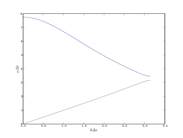
Figure 2: Plot of the dispersion relation for the semi-discrete equations obtained from the $\textrm{P1}_{\textrm{DG}}$-P2 element in one dimension. The eigenspectrum has two branches, with a spectral gap separating small and large eigenvalues. The lower branch is very straight (and hence accurate).

To investigate this gap in the spectrum further, we used this solution to recover the structure of the modes by looking at the eigenvectors of the matrix in equation (11) when $\omega$ takes these values. We normalised the eigenvectors and calculated the magnitude of the difference between $\hat{u}^{+}$ and $\hat{u}^{-}$, which gives a measure of the discontinuity in each mode. Figure 3 illustrates that the level of discontinuity for modes from the lower frequency branch is much lower than for those from the higher frequency branch.

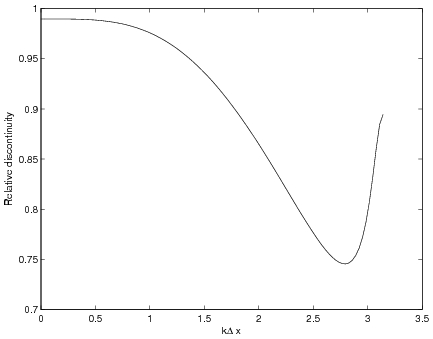
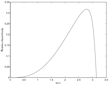
Figure 3: Plots of the magnitude of the discontinuity in $u$ of the eigenmodes for the low (bottom plot) and high (top plot) frequency branches of the dispersion relation. The low frequency modes exhibit low levels of relative discontinuity and the high frequency modes are very discontinuous with the fastest mode being completely out of phase.

4 Analysis of discrete Laplacian for two and three dimensional unstructured meshes

In this section we construct the discrete Laplacian using the $\textrm{P1}_{\textrm{DG}}$-P2 element for unstructured meshes in two and three dimensions and check the eigenvalues for spurious modes. The meshes were produced by Triangle[14] (in two dimensions) and Tetgen[15] (in three dimensions). The matrices $C$, $M^{u}$ and $M^{h}$ were assembled using exact quadrature and the eigenvalues of the discrete Laplacian $(M^{h})^{-1}\sum_{i}C^{T}_{i}(M^{u})^{-1}C_{i}$ were computed numerically using Scientific Python.

4.1 Two dimensions

Table 3 shows the computed eigenvalues for the discrete Laplacian obtained from the $\textrm{P1}_{\textrm{DG}}$-P2 element in two dimensions with Neumann boundary conditions for $\vec{u}$ and Dirichlet boundary conditions for $h$. The meshes are unstructured in a $1\times 1$ square domain.

Max triangle area	Number of elements	vector of eigenvalues in increasing magnitude
0.1	14	$\begin{array}[]{c}[19.44,40.79,44.95,55.42,\\ \qquad 61.42,...,583.7,656.3]\end{array}$
0.05	36	$\begin{array}[]{c}[19.72,48.98,49.16,76.34,\\ \qquad 94.41,...,9102,29160]\\ \end{array}$
0.01	151	$\begin{array}[]{c}[19.73,49.35,49.36,79.02,\\ \qquad 98.80,...126300,2949000]\\ \end{array}$

Table 3: Table showing eigenvalues of the discrete Laplacian obtained from the $\textrm{P1}_{\textrm{DG}}$-P2 element pair in two dimensions with Dirichlet boundary conditions. All the eigenvalues correspond to physical modes.

The Dirichlet boundary conditions for $h$ prohibit the constant $h$ solution with eigenvalue zero and so the smallest physical eigenvalue is $2\pi^{2}$ corresponding to $h=\sin(x)\sin(y)$. It is clear from the table that there are no spurious eigenvalues i.e. eigenvalues that scale with the mesh size, and all of the eigenvalues correspond to physical modes.

Table 4 shows the computed eigenvalues for the discrete Laplacian obtained from the $\textrm{P1}_{\textrm{DG}}$-P2 element in two dimensions with Neumann boundary conditions for $h$ and Dirichlet boundary conditions for $\vec{u}$, on the same $1\times 1$ domain.

Max triangle area	Number of elements	vector of eigenvalues in increasing magnitude
0.1	14	$\begin{array}[]{c}[0.00,9.89,9.90,19.90,\\ \qquad 41.22,...,830.0,960.9]\\ \end{array}$
0.05	36	$\begin{array}[]{c}[0.00,9.88,9.88,19.80,\\ \qquad 40.43,...,15870,41690]\\ \end{array}$
0.01	151	$\begin{array}[]{c}[0.00,9.87,9.87,19.74,\\ \qquad 39.50,...,177300,3274000]\\ \end{array}$

Table 4: Table showing eigenvalues of the discrete Laplacian obtained from the $\textrm{P1}_{\textrm{DG}}$-P2 element pair in two dimensions with Neumann boundary conditions. All the eigenvalues correspond to physical modes.

The Neumann boundary conditions for $h$ admit the constant $h$ solution with eigenvalue zero. The next two physical eigenfunctions are $\sin(\pi x)$ and $\sin(\pi y)$ which both have eigenvalues $\pi^{2}$. There are no spurious eigenvalues.

4.2 Three dimensions

Table 5 shows the computed eigenvalues for the discrete Laplacian obtained from the $\textrm{P1}_{\textrm{DG}}$-P2 element in three dimensions with Neumann boundary conditions for $\vec{u}$ and Dirichlet boundary conditions for $h$. The meshes are unstructured in a $1\times 1\times 1$ cubic domain.

Max tetrahedral volume	Number of elements	vector of eigenvalues in increasing magnitude
0.1	44	$\begin{array}[]{c}[0.00,0.00,0.00,0.00,0.00,\\ \qquad 29.876,...,939.7,1045]\\ \end{array}$
0.01	215	$\begin{array}[]{c}[0.00,0.00,0.00,0.00,0.00,\\ \qquad 0.00,29.87,...,5177,5753]\\ \end{array}$
0.0059	329	$\begin{array}[]{c}[0.00,0.00,0.00,29.71,\\ \qquad 59.85,...,5772,6723]\end{array}$
0.00585	330	$\begin{array}[]{c}[29.72,59.88,60.06,\\ \qquad 60.07,...,5763,6631]\\ \end{array}$
0.005	398	$\begin{array}[]{c}[29.72,59.88,60.06,\\ \qquad 60.07,...,7474,11570]\\ \end{array}$
0.004	487	$\begin{array}[]{c}[29.70,59.80,59.87,59.96,\\ \qquad 90.77,...,10680,12800]\\ \end{array}$
0.003	681	$\begin{array}[]{c}[29.67,59.57,59.61,59.66,\\ \qquad 90.15,...,11610,12350]\\ \end{array}$

Table 5: Table showing eigenvalues of the discrete Laplacian obtained from the $\textrm{P1}_{\textrm{DG}}$-P2 element pair in three dimensions with Dirichlet boundary conditions. There are spurious eigenvalues for the coarsest meshes which disappear when there are more elements and the ratio of $\vec{u}$ DOF to $h$ DOF is greater.

As in the two-dimensional case, the Dirichlet boundary conditions for $h$ prohibit the constant $h$ solution with eigenvalue zero and so the smallest physical eigenvalue is $3\pi^{2}$ corresponding to $h=\sin(x)\sin(y)\sin(z)$. Table 5 shows that spurious eigenvalues are present for very coarse meshes but are not present when the number of elements is increased.

Table 6 shows the computed eigenvalues for the discrete Laplacian obtained from the $\textrm{P1}_{\textrm{DG}}$-P2 element in three dimensions with Neumann boundary conditions for $h$ and Dirichlet boundary conditions for $\vec{u}$. The meshes are unstructured in a $1\times 1\times 1$ cubic domain.

Max tetrahedral volume	Number of elements	vector of eigenvalues in increasing magnitude
0.1	44	$\begin{array}[]{c}[0.00,9.93,9.93,10.06,\\ \qquad 20.15,...,984,1097]\\ \end{array}$
0.01	215	$\begin{array}[]{c}[0.00,9.88,9.88,9.89,\\ \qquad 19.83,...,5385,5931]\\ \end{array}$
0.005	398	$\begin{array}[]{c}[0.00,9.874,9.874,9.875,\\ \qquad 19.78,...,7746,12070]\\ \end{array}$
0.004	487	$\begin{array}[]{c}[0.00,9.873,9.873,9.873,\\ \qquad 19.78,...,10780,13010]\\ \end{array}$
0.003	681	$\begin{array}[]{c}[0.00,9.872,9.872,9.873,\\ \qquad 19.76,...,11600,12330]\\ \end{array}$

Table 6: Table showing eigenvalues of the discrete Laplacian obtained from the $\textrm{P1}_{\textrm{DG}}$-P2 element pair in three dimensions with Neumann boundary conditions. All the eigenvalues correspond to physical modes, indicating that the element pair is stable.

The Neumann boundary conditions for $h$ admit the constant $h$ solution with eigenvalue zero. The next three physical eigenfunctions are $\sin(\pi x)$, $\sin(\pi y)$ and $\sin(\pi z)$ which both have eigenvalues $\pi^{2}$. There are no spurious eigenvalues.

5 Numerical test for the wave equation

In this section we test the $\textrm{P1}_{\textrm{DG}}$-P2 element as applied to the wave equation in two dimensions, with the aim of checking that spurious oscillations do not appear and that the solution remains smooth.

We discretised the equations in time using the Störmer-Verlet method given by

$$M^{u}\frac{{\mathrm{u}}_{i}^{n+1/2}-{\mathrm{u}}_{i}^{n}}{2\Delta t} = -C_{i}{\mathrm{h}}^{n},i=1,\ldots d,$$

$$M^{h}\frac{{\mathrm{h}}^{n+1}-h^{n}}{\Delta t} = \sum_{i=1}^{d}C^{T}_{i}{\mathrm{u}}^{n+1/2},$$

$$M^{u}\frac{{\mathrm{u}}_{i}^{n+1}-{\mathrm{u}}_{i}^{n+1/2}}{2\Delta t} = -C_{i}{\mathrm{h}}^{n+1},i=1,\ldots d,$$

This method is second-order in time, and is symplectic, one of the consequences of which is that there exists a conserved energy which is equal to the exact spatially discretised energy plus a correction of magnitude $\mathcal{O}(\Delta t^{2})$ (see [10] for a review of the Störmer-Verlet method applied to PDEs). This means that small-scale energy will not be dissipated and it provides a good test of the spatial discretisation. As this method is explicit, there is a numerical CFL condition which requires that the fastest oscillation in the system, corresponding to the largest eigenvalue of the discrete Laplacian, should be resolved in time. This discretisation still requires linear systems to be solved to obtain $\vec{u}$ and $h$ at the next time level, although the mass matrix for $\vec{u}$ is block diagonal (with one block per element).

Simulation results are given in figure 4. These results show that the solutions remain smooth and that there are no spurious modes polluting the solution. This good behaviour arises from the stability of the $\textrm{P1}_{\textrm{DG}}$-P2 element.

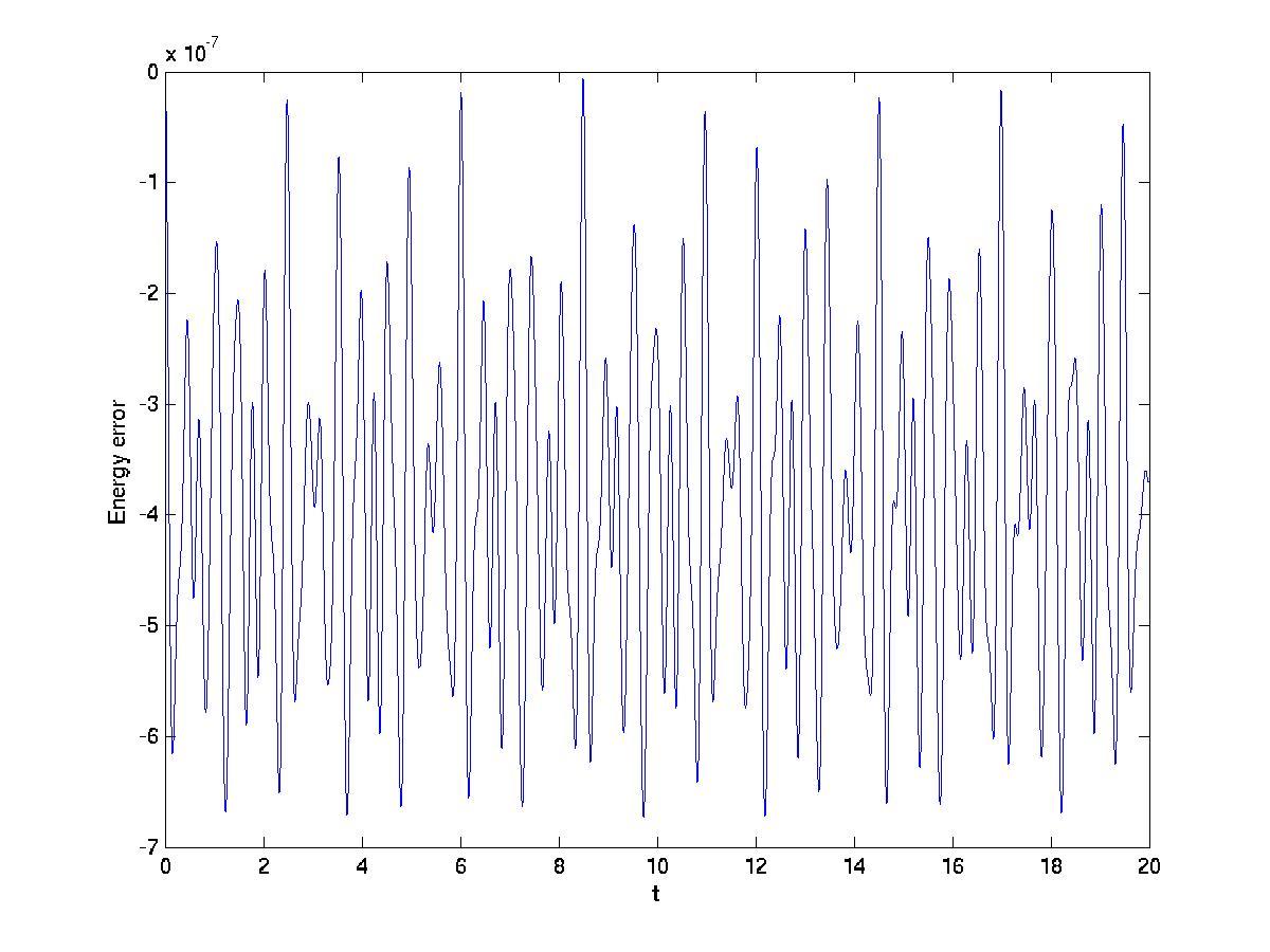
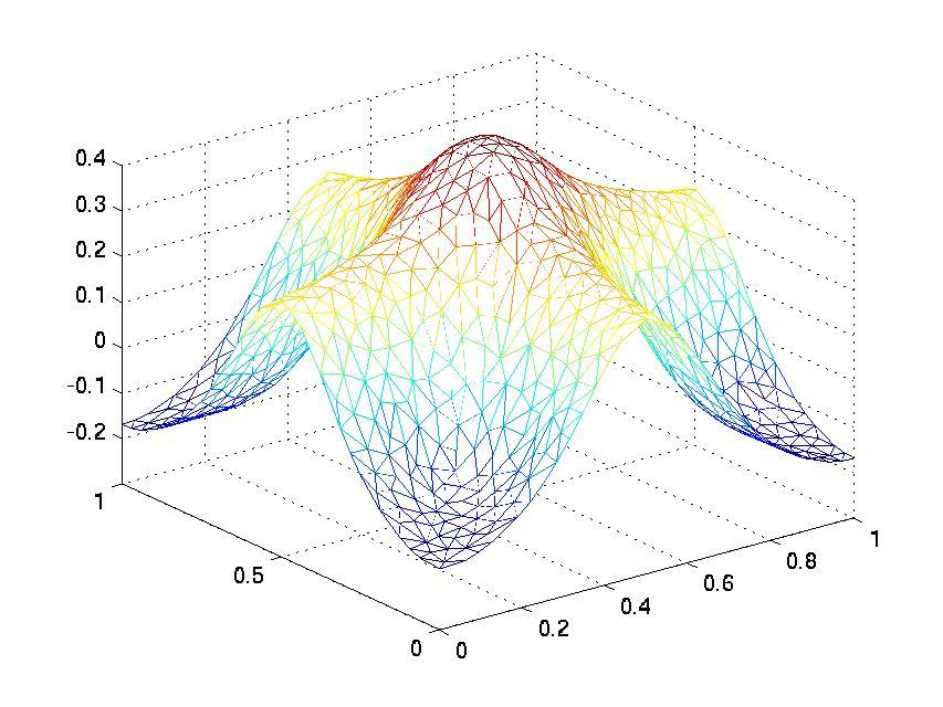
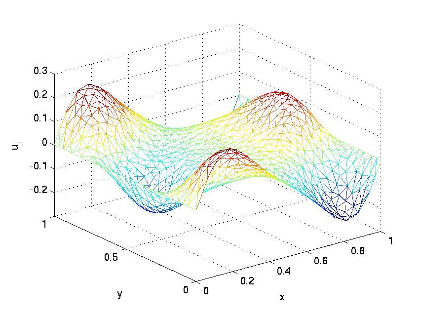
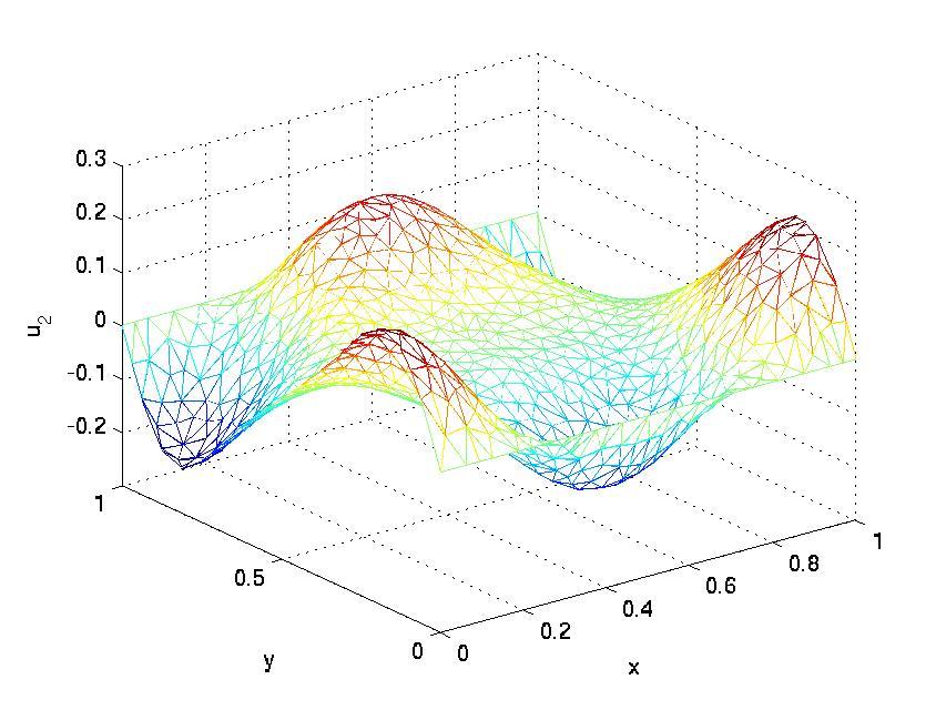
Figure 4: Numerical results obtained from solving the 2-dimensional wave equation in a square domain of area 1 with an unstructured grid with triangular elements of typical area 0.001. The wave speed is $c=1$ and the timestep is $\Delta t=0.001$. Top-left: plot of energy error against time. Top-right: plot of $h$ at time $t=20.0$. Bottom-left and bottom-right: plots of the $x$- and $y$-components of $\vec{u}$. These results show that the numerical solution stays smooth after a large number of timesteps, which is a good indicator that the method is stable. Although it appears from the plot that $\vec{u}$ remains almost continuous, small discontinuities are present in the solution.

6 Summary and Outlook

In this paper we introduced the $\textrm{P1}_{\textrm{DG}}$-P2 mixed element which has discontinuous velocity and continuous pressure. This choice means that the number of DOF for velocity can be increased in order to obtain a stable element. In section 2 we described the construction of the element in one, two and three dimensions and gave example values for the $\vec{u}$ and $h$ DOF. In future implementations in the three-dimensional non-hydrostatic Imperial College Ocean Model (ICOM) [12] we will investigate the relative merits of $\textrm{P1}_{\textrm{DG}}$-P2, $\textrm{P1}_{\textrm{DG}}$-P3, $\textrm{P2}_{\textrm{DG}}$-P3 and other combinations, including augmenting the $\vec{u}$ space with bubble functions, in practical applications.

In section 3 we gave a linear normal mode analysis for the element on a regular grid in one dimension with periodic boundary conditions which showed that the element is stable in this case. The dispersion relation is monotonically increasing with a spectral gap between the two branches, and the lower frequency branch has relatively continuous eigenfunctions with almost continuous eigenfunctions at the lowest frequencies.

In section 4 we presented calculations of eigenvalues of the discrete Laplace matrix obtained from unstructured meshes in two and three dimensions which demonstrated that the element is stable in these cases. In section 5 we presented results from a wave equation calculation on a two dimensional grid which demonstrated that the solutions stay smooth for relatively long time intervals.

This type of element with discontinuous velocity and continuous pressure has some other properties that may make it favourable for use in geophysical codes such as ICOM. The discontinuous element for velocity means that the discretisation locally conserves momentum, and the use of upwinding and flux-limiting means that the discretisation allows a good treatment of advection (see, for example, [11]). As the mass matrix for $\vec{u}$ is block diagonal, the $\sum_{i}C^{T}_{i}(M^{u})^{-1}C_{i}$ matrix remains sparse and so it is not necessary to lump the mass matrix. This makes the discretisation more accurate and reduces problems with balancing various lumped and non-lumped terms.

A key issue with modelling large-scale rotating geophysical flow is that of geostrophic balance, which states that the Coriolis term is nearly balanced by the horizontal pressure gradients:

$$\vec{\Omega}\times\vec{u}\approx-\nabla_{H}p,$$

where $\vec{\Omega}$ is the Earth’s rotation vector and $\nabla_{H}$ is the horizontal gradient. For an element pair such as P1-P1, the pressure gradients are piecewise constant whilst the Coriolis force is piecewise linear and it is not possible to find a pressure field to accurately represent this balance. This leads to pressure gradient errors which pollute the solution after short times, and it becomes necessary to subtract out the balanced pressure (discretised on a higher-order element) in order for the solution to stay near to balance. For the $\textrm{P1}_{\textrm{DG}}$-P2 element pair, the velocity field is piecewise linear whilst the pressure field is piecewise quadratic, and it will be possible to find a pressure field which represents this balance as long as the velocity field remains relatively continuous. The study of discontinuity in the normal modes for the one-dimensional element is encouraging as it shows that the lower branch of the spectrum, corresponding to well-resolved solutions, remains relatively continuous. We will investigate the pressure gradient errors arising from this discretisation in future work.

References

- [1] M. Ainsworth, P. Monk, W. Muniz, Dispersive and dissipative properties of discontinuous Galerkin finite element methods for the second-order wave equation, J. Sci. Comput. 27 (1-3) (2006) 5–40.
- [2] I. Babuska, Error bounds for finite element methods, Numer. Math 16 (1971) 322–333.
- [3] F. Bassi, S. Rebay, A high-order accurate discontinuous finite element method for the numerical solution of the compressible Navier-Stokes equations, J. Comp. Phys. 131.
- [4] F. Brezzi, On the existence, uniqueness and approximation of saddle point problems arising from Lagrangian multiplier, Anal. Num. 8 (1974) 129–151.
- [5] P. M. Gresho, R. L. Sani, Incompressible Flow and the Finite Element Method, Volume 2, Isothermal Laminar Flow, Wiley, 2000.
- [6] M. J. Grote, A. Schneebeli, D. Schotzau, Discontinuous Galerkin finite element method for the wave equation, SIAM Journal on Numerical Analysis 44 (6) (2006) 2408–2431.
- [7] P. Joly, Topics in Computational Wave Propagation: Direct and Inverse Problems, chap. 6, Springer, 2003.
- [8] G. E. M. Karniadakis, S. Sherwin, Spectral/hp Element Methods for Computational Fluid Dynamics, chap. 7, Oxford Science Publications, 2005.
- [9] O. A. Ladyzhenskaya, The mathematical theory of viscous incompressible flow, Gordon and Breach, 1969.
- [10] B. Leimkuhler, S. Reich, Simulating Hamiltonian Dynamics, chap. 12, CUP, 2005.
- [11] J. Levin, M. Iskandarani, D. Haidvogel, To continue or discontinue: Comparisons of continuous and discontinuous Galerkin formulations in a spectral element ocean model, Ocean Modelling 15 (2006) 56–70.
- [12] C. Pain, M. Piggott, A. Goddard, F. Fang, G. Gorman, D. Marshall, M. Eaton, P. Power, C. de Oliveira, Three-dimensional unstructured mesh ocean modelling, Ocean Modelling 10 (2005) 5–33.
- [13] D. L. Roux, A. Sène, V. Rostand, E. Hanert, On some spurious mode issues in shallow-water models using a linear algebra approach, Ocean Modelling (2005) 83–94.
- [14] J. R. Shewchuk, Triangle: engineering a 2D quality mesh generator and Delaunay triangulator, in: M. C. Lin, D. Manocha (eds.), Applied Computational Geometry: Towards Geometric Engineering, vol. 1148 of Lecture Notes in Computer Science, Springer-Verlag, 1996, pp. 203–222, from the First ACM Workshop on Applied Computational Geometry.
- [15] H. Si, K. Gärtner, Meshing piecewise linear complexes by constrained Delaunay tetrahedralizations, in: Proceedings of the 14th International Meshing Roundtable, 2005.