Suppressing noise-induced intensity pulsations in semiconductor lasers by means of time-delayed feedback

Abstract

We investigate the possibility to suppress noise-induced intensity pulsations (relaxation oscillations) in semiconductor lasers by means of a time-delayed feedback control scheme. This idea is first studied in a generic normal form model, where we derive an analytic expression for the mean amplitude of the oscillations and demonstrate that it can be strongly modulated by varying the delay time. We then investigate the control scheme analytically and numerically in a laser model of Lang-Kobayashi type and show that relaxation oscillations excited by noise can be very efficiently suppressed via feedback from a Fabry-Perot resonator.

I Introduction

In many dynamical systems noise plays an important role and influences the system’s properties and the dynamic behavior in a crucial way. Control of the noise-mediated dynamic properties is a central issue in nonlinear science SCH07 .

An often encountered effect of noise is the excitation of irregular stochastic oscillations under conditions where the deterministic system would rest in a stable steady state, e.g., a stable focus. The random fluctuations then push the system out of the steady state. These noise-induced oscillations are a widespread phenomenon and appear, for instance, in lasers PET91 ; DUB99 ; GIA00 ; SHE03 ; USH05 , chemical reaction systems BEA05 , semiconductor devices HIZ06 ; STE05 , neurons LIN04 , and many other systems.

In practical applications the need arises to control the oscillations, for instance, by increasing their coherence and thus the regularity of the oscillations. In recent years different methods to control stochastic systems have been developed, and applied to noise-induced oscillations in a pendulum with a randomly vibrating suspension axis and external periodic forcing LAN97 , stochastic resonance GAM99 ; LIN01 , noise-induced dynamics in bistable delayed systems TSI01 ; MAS02 , and self-oscillations in the presence of noise GOL03 . In the context of coherence resonance GAN93 ; PIK97 , time-delayed feedback in the form originally suggested by Pyragas to stabilize unstable states in deterministic systems PYR92 ; SCH07 has been demonstrated to be a powerful tool to control purely noise-induced oscillations JAN03 . This method couples the difference of the actual state $X(t)\in{\mathbb{R}}^{n}$ and of a delayed state of the system $X(t-\tau)$ back into the system.

$$\frac{d}{dt}X(t)=f(X(t),t)\,-\,K\,[X(t)-X(t-\tau)].$$

The time delay $\tau$ and the (matrix valued) control amplitude $K$ are the control parameters which can be tuned. While previous studies have shown that the delayed feedback method can control the main frequency and the correlation time $t_{cor}$ and thus the regularity of noise-induced oscillations in simple systems JAN03 ; BAL04 ; SCH04b ; POM05a ; POM07 ; PRA07 ; JAN07 as well as in spatially extended systems HIZ05 ; STE05a ; BAL06 , and deteriorate or enhance stochastic synchronization of coupled systems HAU06 , in this paper we focus on the suppression of stochastic oscillations. We analyse the mean amplitude (or, more generally, the covariance) of the oscillations and show that time-delayed feedback control can decrease the mean oscillation amplitude for appropriately chosen delay time, and thus suppress the oscillations.

The paper is organized as follows. In section II we study a generic model consisting of a damped harmonic oscillator driven by white noise and investigate the influence of delayed feedback. In this generic system we derive an analytic expression for the mean square oscillation amplitude in dependence on the feedback and show how the oscillations can be suppressed. In section III we consider a semiconductor laser, a practically relevant example, and show how optical feedback from a Fabry-Perot resonator, which realizes the delayed-feedback scheme, can suppress noise-induced relaxation oscillations in the laser.

II Generic model

We consider a damped harmonic oscillator (whose fixed point is a stable focus) subject to noise ($\xi$) and feedback control

$$\dot{z}(t) = (\lambda-i\omega_{0})\,z(t)+D\xi(t)\qquad(z\in\mathbb{C})$$

$$-K\,[z(t)-z(t-\tau)],$$

where $\lambda<0$ and $\omega_{0}$ are the damping rate and the natural frequency of the oscillator, respectively, $D$ is the noise amplitude, $K$ is the (scalar) feedback strength and $\tau$ is the delay time of the control term. We consider Gaussian white noise

$$\xi(t) = \xi_{1}(t)+i\xi_{2}(t),\qquad(\xi_{i}\in\mathbb{R})$$

$$\langle\xi_{i}\rangle = 0,$$

$$\langle\xi_{i}(t)\,\xi_{j}(t^{\prime})\rangle = \delta_{ij}\delta(t-t^{\prime}).$$

In our particular system the delay term in eq.(II) does not induce any local bifurcations in the deterministic system. Thus, the fixed point is stable for all $\tau$ and $K$.

A similar normal form (without noise) was previously used to study the stabilization of unstable deterministic fixed points by time-delayed feedback HOE05 , which is possible in the same way as stabilization of unstable deterministic periodic orbits SCH07 ; BAB02 ; BEC02 ; FIE07 .

The power spectral density of $z$ has been calculated in POM05a and is given by (see Fig. 2)

$$S(\omega)=\frac{D^{2}}{2\pi}\frac{1}{[\lambda-K(1-\cos(\omega\tau)]^{2}+[\omega-\omega_{0}+K\sin(\omega\tau)]^{2}}.$$

Figs. 1 and 2 display the dependence of the power spectral density on the delay time. With increasing delay new peaks appear in the spectrum. These are related to new modes generated by the delay as will be shown later.

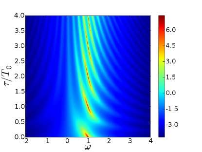
Figure 1: (color online) Power spectral density $S$ as a function of the frequency $\omega$ and the delay time $\tau$ (logarithmic color scale). Parameters: $\lambda=-0.01$, $\omega_{0}=1$ ($T_{0}=2\pi$), $D=1$, $K=0.2$

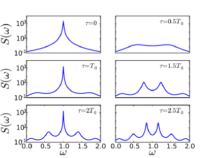
Figure 2: (color online) Power spectral density $S(\omega)$ for different delay times $\tau$. Parameters: $\lambda=-0.01$, $\omega_{0}=1$, $D=1$, $K=0.2$

Before proceeding, we transform eq.(II) into a rotating frame $z(t)=u(t)\,e^{-i\omega_{0}t}$

$$\dot{u}(t) = (\lambda-K)\,u(t)+K\,e^{i\omega_{0}\tau}u(t-\tau)+e^{i\omega_{0}t}D\,\xi(t)$$ (2)

$$= a\,u(t)+b\,u(t-\tau)+D\,\tilde{\xi}(t),$$

where $a\in\mathbb{R}$, $b\in\mathbb{C}$, and $\tilde{\xi}(t)=e^{i\omega_{0}t}\xi(t)$ is a noise term with the same properties as $\xi(t)$. The purpose of the transformation is to make the parameter $a$ real, which will be necessary later.

In KUE92 Küchler and Mensch analyzed equation (2) for real variables. We will follow their approach and adapt it to complex variables. Similar results for the Van der Pol oscillator have been obtained independently in POT07 . A different two-dimensional system with noise and delay has been recently studied in PAT06 .

We will calculate the autocorrelation function

$$G(t)=\langle u(s+t)\,\overline{u(s)}\rangle$$

in an interval $t\in[0,\tau]$, where the overbar denotes complex conjugate. In particular, this gives the mean square amplitude $\langle r^{2}\rangle=\langle|z|^{2}\rangle=\langle|u|^{2}\rangle=G(0)$ of the oscillations. With the Green’s function $u_{0}(t)$ solving

$$\dot{u}_{0}(t)-a\,u_{0}(t)-bu_{0}(t-\tau)=\delta(t),$$

with $u_{0}(t)=0$ for $t<0$, we can formally find a solution of equation (II)

$$u(t)=\int\limits_{-\infty}^{t}\!\mathrm{d}t_{1}\,u_{0}(t-t_{1})\,D\,\tilde{\xi}(t_{1}).$$ (3)

Using (3) we obtain

$$G(t) = \langle u(\tilde{t}+t)\,\overline{u(\tilde{t})}\rangle$$

$$= D^{2}\int\limits_{-\infty}^{\tilde{t}+t}\!dt_{1}\,\int\limits_{-\infty}^{\tilde{t}}\!dt_{2}\,u_{0}(\tilde{t}+t-t_{1})\,\overline{u_{0}(\tilde{t}-t_{2})}$$

$$\times\langle\tilde{\xi}(t_{1})\,\overline{\tilde{\xi}(t_{2})}\rangle$$

$$\stackrel{{\scriptstyle s=\tilde{t}-t_{1}}}{{=}} 2D^{2}\,\int\limits_{0}^{\infty}\!ds\,u_{0}(s+t)\,\overline{u_{0}(s})$$

$$\equiv 2D^{2}\,C(t).$$

The Green’s function $u_{0}$ can be calculated BUD04 ; KUE92 by iteratively integrating eq. (2) on intervals $[k\,\tau,\,(k+1)\,\tau)$

$$u_{0}(t)=\sum_{k=0}^{\left\lfloor t/\tau\right\rfloor}\frac{b^{k}}{k!}\,(t-k\,\tau)^{k}\,e^{a\,(t-\tau k)}.$$

From the definition of $C$ and $u_{0}$ it follows that $C$ satisfies the following equations

$$C(t) = \overline{C(-t)}$$ (4)

$$\dot{C}(t) = a\,C(t)+b\,C(t-\tau)\qquad(t>0)$$ (5)

$$\dot{C}(t) = a\,C(t)+b\,\overline{C(\tau-t)}\qquad(t>0).$$ (6)

Using these three equations, we can find an ordinary differential equation for $C$, using eqs.(6),(5),

$$\frac{d^{2}}{dt^{2}}\,C(t) = a\,C^{\prime}(t)-b\,\overline{C^{\prime}(\tau-t)}$$

$$= a\,[a\,C(t)+b\,C(t-\tau)]$$

$$-b\,\overline{[a\,C(\tau-t)+b\,C(-t)]}$$

$$= a^{2}C(t)+a\,b\,C(t-\tau)$$

$$-a\,b\,\overline{C(t-\tau)}-|b|^{2}\overline{C(-t)}$$

$$= (a^{2}-|b|^{2})\,C(t).$$

Here it was necessary to have a real $a$, in order for the delay terms to cancel. Thus $C$ is of the form

$$C(t)=A\,e^{\Lambda t}+B\,e^{-\Lambda t},$$

with

$$\Lambda=\sqrt{a^{2}+|b|^{2}}=\sqrt{(\lambda-K)^{2}-K^{2}}.$$

The complex coefficients $A$ and $B$ can be found from the equations

$$C(0) = \overline{C(0)}\in\mathbb{R},$$ (7)

$$\dot{C}(0) = a\,C(0)+b\,\overline{C(\tau)}$$ (8)

and

$$-1 = \int\limits_{0}^{\infty}\!ds\,\frac{d}{ds}\,[u_{0}(s)\,\overline{u_{0}(s)}]$$

$$= \int\limits_{0}^{\infty}\!ds\,[\dot{u}_{0}(s)\,\overline{u_{0}(s)}+u_{0}(s)\,\overline{\dot{u}_{0}(s)}]$$

$$= a\,C(0)+b\,\overline{C(\tau)}+a\,C(0)+\overline{b}\,C(\tau).$$

Solving equations (7),(8) and (II) for $A$ and $B$ gives the mean square oscillation amplitude

$$C(0) = \langle r^{2}\rangle=\mathrm{Re}(A)+\mathrm{Re}(B)$$ (10)

$$= -\frac{1}{4\Lambda}\cdot\frac{K^{2}+2\Lambda^{2}-K^{2}\cosh(2\Lambda\tau)}{K\,\cosh(\Lambda\tau)\,[\Lambda\cos(\omega_{0}\tau)+K\,\sinh(\Lambda\tau)]+a\,[\Lambda+K\cos(\omega_{0}\tau)\,\sinh(\Lambda\tau)]}.$$

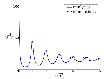
Figure 3: (color online) Mean square amplitude $\langle r^{2}\rangle$ of noise-induced oscillations (solid line: analytics, dots: numerics). Parameters: $\lambda=-0.01$, $D=1$, $K=0.2$, $\omega_{0}=1$ ($T_{0}=2\pi$)

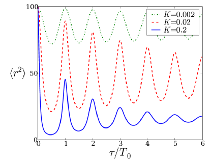
Figure 4: (color online) Mean square amplitude $\langle r^{2}\rangle$ of oscillations as a function of the delay time $\tau$ for different $K$ (analytic solution). Parameters: $\lambda=-0.01$, $D=1$, $\omega_{0}=1$ ($T_{0}=2\pi$)

This is now an analytic result which allows to analyze the effect of the control term. Figure 3 displays analytic and numeric results for the oscillation amplitude. The dependence on the control force $K$ is shown in Fig. 4.

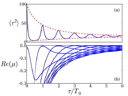
Figure 5: (color online) (a) Mean square amplitude $\langle r^{2}\rangle$ of oscillations and (b) real part of the eigenvalue spectrum of the fixed point as a function of the delay time $\tau$. The dashed lines in (a) mark the envelope $C_{\pm}$. Parameters: $\lambda=-0.01$, $D=1$, $K=0.2$, $\omega_{0}=1$ ($T_{0}=2\pi$)

The oscillation amplitude can thus be strongly modulated by varying $\tau$. We can obtain the envelopes of the modulation by setting the terms $\cos(\omega_{0}\tau)$ to their maximum and minimum values $\pm 1$ in eq.(10)

$$C_{\pm}=\frac{1}{2\Lambda}\cdot\frac{K\sinh(\Lambda\tau)\mp\Lambda}{K\cosh(\Lambda\tau)\pm a}.$$

Figure 5(a) displays $\langle r^{2}\rangle$ and the envelopes versus $\tau$. The mean square oscillation amplitude is modulated as a function of $\tau$ with a period $T_{0}=2\pi/\omega_{0}$. The maxima and minima occur at

$$\tau_{+}=n\,T_{0}\quad\mbox{and}\quad\tau_{-}=\frac{2n+1}{2}\,T_{0}$$

respectively. The smallest oscillation amplitude is reached at

$$\tau_{opt}=T_{0}/2.$$

To understand the behavior of the mean square oscillation amplitude as a function of the delay time $\tau$, one has to look at the eigenvalue spectrum of the fixed point $z=0$ of eq. (II) (without fluctuations). The ansatz $z(t)\propto e^{\mu t}$ in eq. (II) gives rise to a transcendental equation for the eigenvalues $\mu$:

$$\mu=(\lambda-i\omega_{0}-K)+K\,e^{-\mu\tau}.$$ (11)

This equation can be solved using the Lambert function. The Lambert function W is defined AMA05 as the inverse $W(z)$ of the equation

$$W\,e^{W}=z\qquad(z\in\mathbb{C}).$$ (12)

Since eq.(12) has infinitely many solutions, the Lambert function W has infinitely many branches $W_{n}(z)$ indexed by $n$. Using the Lambert function W the solutions of (11) are given by

$$\tau\mu_{n}=W_{n}[\tau\,K\,e^{-(\lambda-i\omega_{0}-K)\tau}]+(\lambda-i\omega_{0}-K)\tau.$$

Fig 5(b) shows the real part of the spectrum versus $\tau$. As $\tau$ increases, different eigenvalue branches originating from $-\infty$ approach the zero axis (albeit remaining $<0$) and then bend away again. Since the real part of the eigenvalues corresponds to the damping rate of the respective mode, the oscillation amplitude excited by noise is large if a mode is weakly damped, and small if all modes have rather large (negative) damping rates.

Because eq. (II) is linear and $\xi$ is Gaussian noise, the probability distribution $p(x,y)$, where $z=x+iy$, is also a Gaussian distribution PAT06 . The rotational invariance ($z^{\prime}=z\,e^{i\phi}$) of eq. (II) implies, that $p(x,y)$ is invariant under rotations, too. These two arguments lead to the probability distribution

$$p(x,y)=\frac{1}{2\pi}\sqrt{\frac{1}{\sigma_{x}^{2}\,\sigma_{y}^{2}}}\,\exp\left[-\frac{x^{2}}{2\sigma_{x}^{2}}-\frac{y^{2}}{2\sigma_{y}^{2}}\right],$$

with

$$\sigma_{x}^{2}=\sigma_{y}^{2}=\frac{1}{2}\langle r^{2}\rangle.$$

Figure 6 shows the marginal distribution

$$p(x)=\int\limits_{-\infty}^{\infty}\!\mathrm{d}y\,p(x,y)$$

for $\tau=0$ (dashed) and $\tau=\tau_{opt}=T_{0}/2$ (solid). The case $\tau=0$ corresponds to no control, because the feedback term in (II) vanishes. The case $\tau=\tau_{opt}$ realizes the optimal delay time, where the oscillations are most strongly suppressed and the distribution $p(x,y)$ is narrowest.

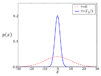
Figure 6: (color online) Marginal probability distribution $p(x)$ without ($\tau=0$) and with optimal control ($\tau=T_{0}/2$) Parameters: $\lambda=-0.01$, $K=0.2$, $D=1$,$\omega_{0}=1$ ($T_{0}=2\pi$)

III Laser model

In this section we investigate the effects of feedback and noise in a semiconductor laser. A laser with feedback from a conventional mirror can be described by the Lang-Kobayashi equations LAN80b . Other types of feedback have also been investigated AGR92 ; ERZ06 . One particular feedback realizes the delayed feedback control with an all-optical scheme TRO06 ; SCH06a . The feedback is here generated by a Fabry-Perot resonator. A schematic view of this setup is shown in Fig. 7. A fraction of the emitted laser light is coupled into a resonator. The resonator then feeds an interference signal of the actual electric field $E(t)$ and the delayed (by the round trip time) electric field $E(t-\tau)$ back into the laser.

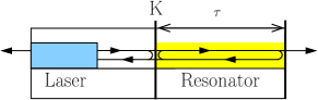
Figure 7: (color online) Setup of a laser coupled to a Fabry-Perot resonator realizing the time-delayed feedback control

A modified set of non-dimensionalized ALS96 Lang-Kobayashi equations TRO06 describes this setup

$$\frac{d}{dt}E = \frac{1}{2}(1+i\,\alpha)\,n\,E$$

$$-e^{i\varphi}K\,[E(t)-e^{i\psi}E(t-\tau)]+F_{E}(t),$$

$$T\,\frac{d}{dt}n = p-n-(1+n)\,|E|^{2},$$

where the variables and parameters are defined in Table 1.

$E$	complex field amplitude
$n$	carrier density
$\alpha$	linewidth enhancement factor
$K$	feedback strength
$\tau$	roundtrip time in the Fabry-Perot
$p$	excess pump injection current
$T$	timescale parameter
$F_{E}$	noise term describing spontaneous emission
$\beta$	spontaneous emission factor
$n_{0}$	threshold carrier density
$\varphi,\psi$	phases depending on the mirror positions

Table 1: Nondimensionalized laser variables and parameters

The phases $\varphi$ and $\psi$ depend on the sub-wavelength positioning of the mirrors. By precise tuning $\varphi=2\pi n$ and $\psi=2\pi m$ one can realize the usual Pyragas feedback control

$$-K\,[E(t)-E(t-\tau)].$$

We consider small feedback strength $K$, so that the laser is not destabilized and no delay-induced bifurcations occur. A sufficient condition TRO06 is that

$$K<K_{c}=\frac{1}{\tau\sqrt{1+\alpha^{2}}}.$$

The noise term $F_{E}$ in (III) arises from spontaneous emission, and we assume the noise to be white and Gaussian

$$\langle F_{E}\rangle=0,\qquad\langle F_{E}(t)\,\overline{F_{E}(t^{\prime})}\rangle=R_{sp}\delta(t-t^{\prime}),$$

with the spontaneous emission rate

$$R_{sp}=\beta(n+n_{0}).$$

where $\beta$ is the spontaneous emission factor, and $n_{0}$ is the threshold carrier density. Without noise the laser operates in a steady state (continuous wave cw emission). To find these steady state values, we transform eqs. (III) into equations for intensity $I$ and phase $\phi$ by $E=\sqrt{I}\,e^{i\phi}$ (see Appendix A):

$$\frac{d}{dt}I = n\,I-2K\,[I-\sqrt{I}\sqrt{I_{\tau}}\,\cos(\phi_{\tau}-\phi)]+R_{sp}+F_{I}(t),$$

$$\frac{d}{dt}\phi = \frac{1}{2}\alpha\,n+K\,\frac{\sqrt{I_{\tau}}}{\sqrt{I}}\,\sin(\phi_{\tau}-\phi)+F_{\phi}(t),$$ (14)

$$T\,\frac{d}{dt}n = p-n-(1+n)\,I,$$

where $I_{\tau}=I(t-\tau)$, $\phi_{\tau}=\phi(t-\tau)$, and

$$\langle F_{I}\rangle=0, \langle F_{\phi}\rangle=0,$$

$$\langle F_{I}(t)\,F_{\phi}(t^{\prime})\rangle =0,$$

$$\langle F_{I}(t)\,F_{I}(t^{\prime})\rangle = 2R_{sp}\,I\,\delta(t-t^{\prime})$$

$$\langle F_{\phi}(t)\,F_{\phi}(t^{\prime})\rangle = \frac{R_{sp}}{2I}\,\delta(t-t^{\prime}).$$

Setting $\frac{d}{dt}I=0$, $\frac{d}{dt}n=0$, $\frac{d}{dt}\phi=\mathrm{const}$, $K=0$ and replacing the noise terms by their mean values, gives a set of equations for the mean steady state solutions $I_{*},$ $n_{*}$ and $\phi=\omega_{*}t$ without feedback (the solitary laser mode). Our aim is now to analyze the stability (damping rate) of the steady state. A high stability of the steady state, corresponding to a large damping rate, will give rise to small-amplitude noise-induced relaxation oscillations whereas a less stable steady state gives rise to stronger relaxation oscillations. Linearizing eqs. (14) around the steady state $X(t)=X_{*}+\delta X(t)$, with $X(t)=(I,\,\phi,\,n)$ gives

$$\frac{d}{dt}X(t)=U\,X(t)-V\,[X(t)-X(t-\tau)]+F(t),$$ (15)

with

$$U = \left[\begin{array}[]{ccc}n_{*}-\Gamma_{I}&0&I_{*}+\beta\\ 0&0&\frac{1}{2}\alpha\\ -\frac{1}{T}(1+n_{*})&0&-\frac{1}{T}(1+I_{*})\end{array}\right],$$

$$V = \mathrm{diag}(K,\,K,\,0)$$

where $diag(...)$ denotes a $3\times 3$ diagonal matrix, and

$$F=(F_{I},\,F_{\phi},\,0).$$

The Fourier transform of eq.(15) gives

$$\widehat{X}(\omega)=\underbrace{[i\omega-U+V\,(1-e^{-i\omega\tau})]^{-1}}_{\equiv M}\,\widehat{F}(\omega).$$

The Fourier transformed covariance matrix of the noise is

$$\langle\widehat{F}(\omega)\,\widehat{F}(\omega^{\prime})^{\dagger}\rangle=\frac{1}{2\pi}\mathrm{diag}(2R_{sp}I_{*},\,\frac{R_{sp}}{2I_{*}},\,0)\,\delta(\omega-\omega^{\prime}),$$

with the adjoint $\dagger$. The matrix-valued power spectral density $S(\omega)$ can then be defined through

$$S(\omega)\,\delta(\omega-\omega^{\prime})=\langle\widehat{X}(\omega)\,\widehat{X}(\omega)^{\dagger}\rangle$$

and is thus given by

$$S(\omega) = \mathrm{diag}\left(S_{\delta I}(\omega),\,S_{\delta\phi}(\omega),\,S_{\delta n}(\omega)\right)$$

$$= \frac{1}{2\pi}\,M\,\mathrm{diag}(2R_{sp}I_{*},\,\frac{R_{sp}}{2I_{*}},\,0)\,M^{\dagger}.$$

The frequency power spectrum is related to the phase power spectrum $S_{\delta\phi}(\omega)$ by AGR93

$$S_{\delta\dot{\phi}}(\omega)=\omega^{2}\,S_{\delta\phi}(\omega).$$

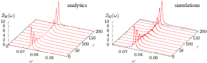
Figure 8: (color online) Analytical (left) and numerical (right) results for the power spectral density $S_{\delta I}(\omega)$ of the intensity for different values of the delay time $\tau$.
Parameters: $p=1,\>T=1000,\>\alpha=2,\>\beta=10^{-5},\>n_{0}=10,\>K=0.002$. (A typical unit of time is the photon lifetime $\tau_{p}=10^{-11}s$, corresponding to a frequency of 100 GHz.)

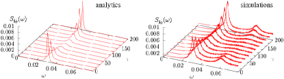
Figure 9: (color online) Analytical (left) and numerical (right) results for the power spectral density $S_{\delta\phi}(\omega)$ of the frequency for different values of the delay time $\tau$.
Parameters: $p=1,\>T=1000,\>\alpha=2,\>\beta=10^{-5},\>n_{0}=10,\>K=0.002$

Figures 8 and 9 display the intensity and the frequency power spectra, respectively, for different values of the delay time $\tau$, obtained analytically from the linearized equations (left) and from simulations of the full nonlinear equations (right). All spectra have a main peak at the relaxation oscillation frequency $\Omega_{RO}\approx 0.03$. The higher harmonics can also be seen in the spectra obtained from the nonlinear simulations. The main peak decreases with increasing $\tau$ and reaches a minimum at

$$\tau_{opt}\approx\frac{T_{RO}}{2}=\frac{2\pi}{2\Omega_{RO}}\approx 100.$$

With further increasing $\tau$ the peak height increases again until it reaches approximately its original maximum at $\tau\approx T_{RO}$. A small peak in the power spectra indicates that the relaxation oscillations are strongly damped. This means that the fluctuations around the steady state values $I_{*}$ and $n_{*}$ are small. Figure 10 displays exemplary time series of the intensity with and without feedback. The time series with feedback show much less pronounced stochastic fluctuations.

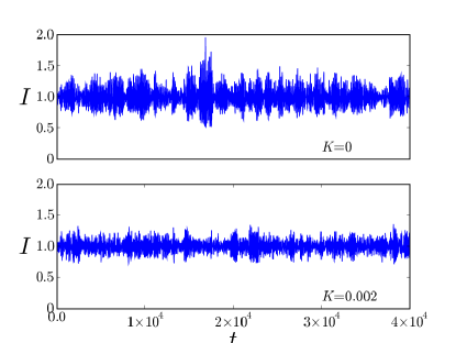
Figure 10: (color online) Intensity time series with (top panel) and without (bottom panel) control
Parameters: $p=1,\>T=1000,\>\alpha=2,\>\beta=10^{-5},\>n_{0}=10,\>\tau=100\approx T_{0}/2$

Next, we study the variance of the intensity distribution as a measure for the oscillation amplitude

$$\Delta I^{2}\equiv\left\langle\left(I-\langle I\rangle\right)^{2}\right\rangle.$$

This measure corresponds to the quantity $\langle r^{2}\rangle$ which we have considered in Section II. Figure 11 displays the variance as a function of the delay time. The variance is minimum at $\tau\approx T_{RO}/2$, thus for this value of $\tau$ the intensity is most steady and relaxation oscillations excited by noise have a small amplitude. This resembles the behavior of the generic model (see Fig. 5(a)).

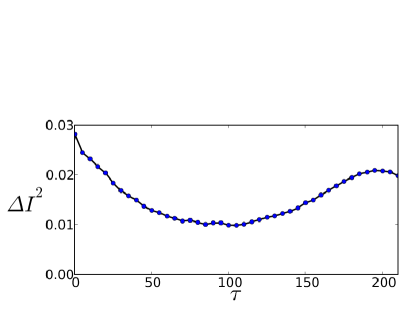
Figure 11: (color online) Variance of the intensity $I$ vs. the delay time. Parameters: $p=1,\>T=1000,\>\alpha=2,\>\beta=10^{-5},\>n_{0}=10,\>K=0.002$

Figure 12 displays the intensity distribution of the laser without (dashed) and with (solid) optimal control (compare Fig. 6). The time-delayed feedback control leads to a narrower distribution and less fluctuations.

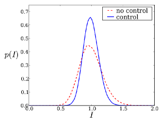
Figure 12: (color online) Probability distribution of the intensity $I$ with and without the resonator (simulations). Parameters: $p=1,\>T=1000,\>\alpha=2,\>\beta=10^{-5},\>n_{0}=10,\>K=0.002$

IV conclusion

In this paper we have shown that time-delayed feedback can suppress noise-induced oscillations.

In the first part we investigated a generic normal form model consisting of a stable focus subject to noise and control. We found an analytic expression for the mean square amplitude of the oscillations. This quantity is modulated with a period of $T_{0}=2\pi/\omega_{0}$ in dependence on $\tau$. For $\tau=T_{0}/2$ the oscillations have the smallest amplitude.

In the second part we considered a semiconductor laser coupled to a Fabry-Perot resonator. In the laser spontaneous emission noise excites stochastic relaxation oscillations. By tuning the cavity round trip time to half the relaxation oscillation period $\tau_{opt}\approx T_{RO}/2$ the oscillations can be suppressed to a remarkable degree. This is demonstrated in the power spectra of the intensity and the frequency, where the relaxation oscillation peak has a minimum height at $\tau_{opt}$. The variance of the intensity distribution $\Delta I$ shows a minimum at $\tau_{opt}$, thus the intensity distribution is narrowest at this value of $\tau$.

Appendix A Ito transformation

Ito’s formula describes how a stochastic differential equation (SDE) is transformed to new coordinates. Consider the stochastic differential equation for $x(t)$

$$dx(t)=a[x(t),t]\,dt+b[x(t),t]\,dW(t).$$

Ito’s formula specifies the transformation to a new variable $y=f(x)$. The SDE for $y$ is given by

$$dy = df[x(t)]$$

$$= a[x(t),t]\,f^{\prime}[x(t)]\,dt+b[x(t),t]\,f^{\prime}[x(t),t]\,dW(t)$$

$$+\frac{1}{2}\,b[x(t),t]^{2}\,f^{\prime\prime}[x(t)]\,dW^{2}.$$

We will apply Ito’s formula to rewrite the laser equations for the complex electric field $E$ in terms of the amplitude $A$ and the phase $\phi$

$$E=A\,e^{i\phi}.$$

The equation for $E$ without feedback is given by

$$\frac{d}{dt}E=\frac{1}{2}(1+i\alpha)\,n\,E+F_{E}(t)$$

or written as a stochastic differential equation

$$dE=\frac{1}{2}(1+i\alpha)\,n\,E\,dt+\sqrt{\frac{R_{sp}}{2}}\,dW(t),$$

with the complex Wiener process $dW=dW_{x}+i\,dW_{y}$. We define the new coordinates

$$\mu+i\phi=\log A+\log e^{i\phi}=\log[E_{x}+i\,E_{y}].$$

Using Ito’s formula with

$$a[E]=\frac{1}{2}(1+i\alpha)\,n\,E,\quad b[E]=\sqrt{\frac{R_{sp}}{2}}\quad\mbox{and},\quad f[E]=\log E,$$

we find

$$d(\mu+i\phi)=\frac{1}{2}(1+i\alpha)\,n\,\frac{1}{E}\,dt-\frac{1}{2}\frac{R_{sp}}{2}\frac{1}{E^{2}}\,dW^{2}+\sqrt{\frac{R_{sp}}{2}}\,\frac{1}{E}\,dW.$$ (17)

For a complex Wiener process $dW$ one can easily see that

$$dW^{2}=[dW_{x}+idW_{y}]^{2}=dW_{x}^{2}+2i\,dW_{x}dW_{y}-dW_{y}^{2}=0.$$

Here we used $dW_{x}^{2}=dW_{y}^{2}=dt$ and $dW_{x}dW_{y}=0$ GAR02 . Thus, equation (17) simplifies to

$$d(\mu+i\phi) = \frac{1}{2}(1+i\alpha)\,n\,\exp(-\mu-i\phi)\,\,dt$$

$$+\sqrt{\frac{R_{sp}}{2}}\,\exp(-\mu-i\phi)\,dW.$$

Splitting this equation into real and imaginary part and transforming with Ito’s formula back to $A=\exp\mu$, we obtain

$$dA = (\frac{1}{2}\,n\,A+\frac{R_{sp}}{4A})dt+\sqrt{\frac{R_{sp}}{2}}\left(\cos\phi\,dW_{x}+\sin\phi\,dW_{y}\right)$$

$$d\phi = \frac{1}{2}\,n\,\alpha\,dt+\frac{1}{A}\sqrt{\frac{R_{sp}}{2}}\left(-\sin\phi\,dW_{x}+\cos\phi\,dW_{y}\right).$$

Because the rotation is an orthogonal transformation, one can understand the increments as new independent Wiener processes

$$dW_{A} = \cos\phi\,dW_{x}+\sin\phi\,dW_{y}$$

$$dW_{\phi} = -\sin\phi\,dW_{x}+\cos\phi\,dW_{y}.$$

We have derived the laser equations in polar coordinates. To include the delay terms does not change the derivation and we will just state the result here

$$\frac{d}{dt}A = \frac{1}{2}nA-K[A-A_{\tau}\cos(\phi_{\tau}-\phi)]+\frac{R_{sp}}{4A}+F_{A}(t)$$

$$\frac{d}{dt}\phi = \frac{1}{2}\alpha n+K\frac{A_{\tau}}{A}\,\sin(\phi_{\tau}-\phi)+F_{\phi}(t)$$

with

$$\langle F_{A}(t)\,F_{A}(t^{\prime})\rangle = \frac{R_{sp}}{2}\,\delta(t-t^{\prime})$$

$$\langle F_{\phi}(t)\,F_{\phi}(t^{\prime})\rangle = \frac{R_{sp}}{2A^{2}}\,\delta(t-t^{\prime}).$$

To obtain the equations for intensity $I=f(A)=A^{2}$ instead of the amplitude Ito’s formula has to be applied again (of course this could be done in one step from the initial equations). The amplitude equation is given by

$$dA = \left\{\frac{1}{2}nA-K[A-A_{\tau}\cos(\phi_{\tau}-\phi)]+\frac{R_{sp}}{4A}\right\}dt$$

$$+\sqrt{\frac{R_{sp}}{2}}\,dW(t).$$

For a real stochastic process $dW$ holds $dW^{2}=dt$. Using Ito’s formula with $dW^{2}=dt$, $f^{\prime}(A)=2A$ and, $f^{\prime\prime}(A)=2$, we find

$$dI = (\frac{1}{2}nA-K[A-A_{\tau}\cos(\phi_{\tau}-\phi)]+\frac{R_{sp}}{4A})2A\,dt$$

$$+\frac{1}{4}R_{sp}2dt+\sqrt{\frac{R_{sp}}{2}}\,2A\,dW(t)$$

and thus

$$\frac{d}{dt}I = nI-K[I-\sqrt{I}\sqrt{I_{\tau}}\cos(\phi_{\tau}-\phi)]$$

$$+R_{sp}+F_{I}(t),$$

with

$$\langle F_{I}(t)\,F_{I}(t^{\prime})\rangle=2R_{sp}I\,\delta(t-t^{\prime}).$$

References

- (1) Handbook of Chaos Control, edited by E. Schöll and H. G. Schuster (Wiley-VCH, Weinheim, 2007), second completely revised and enlarged edition.
- (2) K. Petermann, Laser Diode Modulation and Noise (Kluwer Academic, Boston, 1991).
- (3) J. L. A. Dubbeldam, B. Krauskopf, and D. Lenstra, Phys. Rev. E 60, 6580 (1999).
- (4) G. Giacomelli, M. Giudici, S. Balle, and J. R. Tredicce, Phys. Rev. Lett. 84, 3298 (2000).
- (5) V. V. Sherstnev, A. Krier, A. G. Balanov, N. B. Janson, A. N. Silchenko, and P. V. E. McClintock, Fluct. Noise Lett. 3, 91 (2003).
- (6) O. V. Ushakov, H. J. Wünsche, F. Henneberger, I. A. Khovanov, L. Schimansky-Geier, and M. A. Zaks, Phys. Rev. Lett. 95, 123903 (2005).
- (7) V. Beato, I. Sendiña-Nadal, I. Gerdes, and H. Engel, Phys. Rev. E 71, 035204 (2005).
- (8) G. Stegemann, A. G. Balanov, and E. Schöll, Phys. Rev. E 71, 016221 (2005).
- (9) J. Hizanidis, A. G. Balanov, A. Amann, and E. Schöll, Phys. Rev. Lett. 96, 244104 (2006).
- (10) B. Lindner, J. García-Ojalvo, A. Neiman, and L. Schimansky-Geier, Phys. Rep. 392, 321 (2004).
- (11) P. S. Landa, A. A. Zaikin, M. G. Rosenblum, and J. Kurths, Phys. Rev. E 56, 1465 (1997).
- (12) L. Gammaitoni, M. Löcher, A. Bulsara, P. Hänggi, J. Neff, K. Wiesenfeld, W. Ditto, and M. E. Inchiosa, Phys. Rev. Lett. 82, 4574 (1999).
- (13) J. F. Lindner, J. Mason, J. Neff, B. J. Breen, W. L. Ditto, and A. R. Bulsara, Phys. Rev. E 63, 041107 (2001).
- (14) L. S. Tsimring and A. Pikovsky, Phys. Rev. Lett. 87, 250602 (2001).
- (15) C. Masoller, Phys. Rev. Lett. 88, 034102 (2002).
- (16) D. Goldobin, M. Rosenblum, and A. Pikovsky, Phys. Rev. E 67, 061119 (2003).
- (17) G. Hu, T. Ditzinger, C. Z. Ning, and H. Haken, Phys. Rev. Lett. 71, 807 (1993).
- (18) A. Pikovsky and J. Kurths, Phys. Rev. Lett. 78, 775 (1997).
- (19) K. Pyragas, Phys. Lett. A 170, 421 (1992).
- (20) N. B. Janson, A. G. Balanov, and E. Schöll, Phys. Rev. Lett. 93, 010601 (2004).
- (21) A. G. Balanov, N. B. Janson, and E. Schöll, Physica D 199, 1 (2004).
- (22) E. Schöll, A. G. Balanov, N. B. Janson, and A. Neiman, Stoch. Dyn. 5, 281 (2005).
- (23) J. Pomplun, A. Amann, and E. Schöll, Europhys. Lett. 71, 366 (2005).
- (24) J. Pomplun, A. G. Balanov, and E. Schöll, Phys. Rev. E 75, 040101 (2007).
- (25) T. Prager, H. P. Lerch, L. Schimansky-Geier, and E. Schöll, J. Phys. A (2007), in print.
- (26) N. B. Janson, A. G. Balanov, and E. Schöll, in Handbook of Chaos Control, edited by E. Schöll and H. G. Schuster (Wiley-VCH, Weinheim, 2007), second completely revised and enlarged edition, to be published.
- (27) J. Hizanidis, A. G. Balanov, A. Amann, and E. Schöll, Int. J. Bifur. Chaos 16, 1701 (2006).
- (28) G. Stegemann, A. G. Balanov, and E. Schöll, Phys. Rev. E 73, 016203 (2006).
- (29) A. G. Balanov, V. Beato, N. B. Janson, H. Engel, and E. Schöll, Phys. Rev. E 74, 016214 (2006).
- (30) B. Hauschildt, N. B. Janson, A. G. Balanov, and E. Schöll, Phys. Rev. E 74, 051906 (2006).
- (31) P. Hövel and E. Schöll, Phys. Rev. E 72, 046203 (2005).
- (32) N. Baba, A. Amann, E. Schöll, and W. Just, Phys. Rev. Lett. 89, 074101 (2002).
- (33) O. Beck, A. Amann, E. Schöll, J. E. S. Socolar, and W. Just, Phys. Rev. E 66, 016213 (2002).
- (34) B. Fiedler, V. Flunkert, M. Georgi, P. Hövel, and E. Schöll, Phys. Rev. Lett. 98, 114101 (2007).
- (35) U. Küchler and B. Mensch, Stoch. Rep 40, 23 (1992).
- (36) A. Pototsky and N. B. Janson, Phys. Rev. E (2007), submitted.
- (37) K. Patanarapeelert, T. D. Frank, R. Friedrich, P. J. Beek, and I. M. Tang, Phys. Rev. E 73, 021901 (2006).
- (38) A. Budini and M. O. Cáceres, Phys. Rev. E 70, (2004).
- (39) A. Amann, E. Schöll, and W. Just, Physica A 373, 191 (2007).
- (40) R. Lang and K. Kobayashi, IEEE J. Quantum Electron. 16, 347 (1980).
- (41) G. P. Agrawal and G. R. Gray, Phys. Rev. A 46, 5890 (1992).
- (42) H. Erzgräber, B. Krauskopf, D. Lenstra, A. P. A. Fischer, and G. Vemuri, Phys. Rev. E 73, 055201 (2006).
- (43) V. Z. Tronciu, H. J. Wünsche, M. Wolfrum, and M. Radziunas, Phys. Rev. E 73, 046205 (2006).
- (44) S. Schikora, P. Hövel, H. J. Wünsche, E. Schöll, and F. Henneberger, Phys. Rev. Lett. 97, 213902 (2006).
- (45) P. M. Alsing, V. Kovanis, A. Gavrielides, and T. Erneux, Phys. Rev. A 53, 4429 (1996).
- (46) G. P. Agrawal and N. K. Dutta, Semiconductor Lasers (Van Nostrand Reinhold, New York, 1993).
- (47) C. W. Gardiner, Handbook of Stochastic Methods for Physics, Chemistry and the Natural Sciences (Springer, Berlin, 2002).