Quasi-classical rate coefficient calculations for the rotational (de)excitation of H₂O by H₂

Abstract

Context. The interpretation of water line emission from existing observations and future HIFI/Herschel data requires a detailed knowledge of collisional rate coefficients. Among all relevant collisional mechanisms, the rotational (de)excitation of H₂O by H₂ molecules is the process of most interest in interstellar space.

Aims. To determine rate coefficients for rotational de-excitation among the lowest 45 para and 45 ortho rotational levels of H₂O colliding with both para and ortho-H₂ in the temperature range 20$-$2000 K.

Methods. Rate coefficients are calculated on a recent high-accuracy H₂O$-$H₂ potential energy surface using quasi-classical trajectory calculations. Trajectories are sampled by a canonical Monte-Carlo procedure. H₂ molecules are assumed to be rotationally thermalized at the kinetic temperature.

Results. By comparison with quantum calculations available for low lying levels, classical rates are found to be accurate within a factor of 1$-$3 for the dominant transitions, that is those with rates larger than a few 10^-12cm³s^-1. Large velocity gradient modelling shows that the new rates have a significant impact on emission line fluxes and that they should be adopted in any detailed population model of water in warm and hot environments.

1 Introduction

Since its discovery in interstellar space (Cheung et al. cheung69 (1969)), water vapour has been detected in a great variety of astronomical objects using both Earth-based and, foremost, spacecraft observations. The Infrared Space Observatory (ISO), in particular, has revealed the ubiquity of water in the interstellar (ISM) and circumstellar (CSM) media (for a recent review see Cernicharo & Crovisier cernicharo05 (2005)). The more recent Submillimetre Wave Astronomy Satellite (SWAS) and Odin missions have also measured gaseous water in a wide variety of sources using the single ground-state rotational transitions of ortho-H₂O at 557 GHz (e.g. Melnick & Bergin melnick05 (2005); Hjalmarson et al. hjalmarson03 (2003)). Finally, water is also detected at radio and (sub)millimeter wavelengths through maser transitions which are commonly associated with star-forming regions (e.g. Cernicharo et al. cernicharo90 (1990, 1999); Goddi et al. goddi07 (2007) and references therein or extraglactic sources (e.g. Cernicharo et al. cernicharo06 (2006); Kondratko et al. kondratko06 (2006) and references therein).

The abundance of water varies largely in cold and warm media. In the former, because of the freezing of water onto the dust grains, water does not exceed $\sim 10^{-8}$ (Bergin & Snell bergin02 (2002); Poelman et al. poelman07 (2007) and references therein). But in warm regions, water can become the most abundant molecule after H₂, with an abundance of $\sim 10^{-4}$. In star forming regions, this occurs both because of the release in the gas phase of the grain ices and because of endothermic reactions efficiently forming water in the gas phase (e.g. Ceccarelli et al. ceccarelli96 (1996); Doty & Neufeld doty97 (1997) and references therein). Under these conditions, water becomes a crucial molecule in the thermal and chemical balance. In fact, owing to its large dipole, water lines will dominate the cooling (and sometime even heating) of the gas in a large range of gas densities and temperatures (e.g. Neufeld & Melnick neufeld91 (1991); Ceccarelli et al. ceccarelli96 (1996); Cernicharo et al. cernicharo06 (2006) and references therein). Also, since oxygen will be mostly locked in water molecules at temperatures larger than about 200 K, the chemical abundance of more complex and less abundant molecules will depend on the water abundance.

For all these reasons, water is a key molecule in space, and its observation and the determination of its abundance are critical for many theoretical aspects. Indeed, observing and measuring the water lines and their abundance is an important task for the high resolution spectrometer Heterodyne Instrument for the Far Infrared (HIFI) on board the ESA funded Herschel satellite, which will be launched in 2008. However, as stated by Cernicharo & Crovisier (cernicharo05 (2005)), “little new information will be obtained if collisional rates adapted to the temperatures of the clouds in the ISM and CSM are not available”.

Collisional rate coefficients are indeed essential in the description of the energy exchange processes responsible for molecular line formation in astronomical environments. Spectral features such as maser emission are produced in low-density conditions far from thermodynamic equilibrium and through a complex competition between radiative and collisional processes, including infrared emission from dust (e.g. Poelman et al. poelman07 (2007)). In the ISM and CSM, the main colliding partners are hydrogen molecules, hydrogen and helium atoms, and electrons. In general, however, H₂ is the dominant form of hydrogen and as it is more abundant than He (by a factor of $\sim 5$) and electrons (by $\sim$ 4$-$8 orders of magnitude), H₂ is usually the dominant exciting species. At typical ISM and CSM temperatures ($T<2000$ K), the dominant energy exchange process is thus rotational (de)excitation by H₂, although vibrational excitation cannot be neglected in the highest temperature and density regions.

To the best of our knowledge no experimental state-to-state data is available for H₂O$-$H₂ except for the total relaxation rate of the water bending mode (see Faure et al. 2005a and references therein). On the theoretical side, quantum close-coupling (CC) state-to-state calculations for the rotational excitation of H₂O by H₂ and He have been performed for kinetic temperatures and energy levels lower than 140 K and 2000 K, respectively (Green et al. green93 (1993); Phillips et al. phillips96 (1996); Dubernet et al. dubernet02 (2002); Grosjean et al. grosjean03 (2003); Dubernet et al. dubernet06 (2006)). Hence, current models of water emission in warm and hot environments rely exclusively on rates for excitation by He atoms, usually scaled by the reduced mass ratio $\rm(\mu_{H_{2}O-H_{2}}/\mu_{H_{2}O-He})^{1/2}$ (e.g. Poelman & Spaans poelman05 (2005)). It has been shown by Phillips et al. (phillips96 (1996)), however, that excitation by para-H₂ in its $J$=0 level is not too different from excitation by He atoms (with most rates differing by a multiplicative factor of 1$-$3) but that excitation by H₂ in excited rotational levels is significantly different. This mainly reflects the importance of the long-range interaction between the H₂ quadrupole moment and the dipole of H₂O (Phillips et al. phillips96 (1996)). Rates for excitation of H₂O by H₂ at high temperatures and/or for high rotational levels are therefore urgently needed for the interpretation of existing and future water emission spectra.

In principle, scattering calculations based on the quantum CC method can provide an absolute accuracy of a few percent for a given potential energy surface (PES). As an illustrative example, the recent study of Gilijamse et al. (gilijamse06 (2006)) has shown an excellent agreement between experimentally measured cross sections and CC calculations based on ab initio PES. The major drawback of the quantum CC method is its computational cost which increases dramatically with the number of coupled channels, i.e. with the total energy and the number of degrees of freedom. Very recently, Dubernet et al. (dubernet06 (2006)) provided new rotational rate coefficients for H₂O$-$H₂ at temperatures below 20 K using fully converged CC calculations based on the recent high-accuracy PES of Faure et al. (2005a ). The main objective of their study was to test the influence of the new PES on the scattering calculations and to make comparisons with previous results based on the PES of Phillips et al. (phillips94 (1994)). A significant re-evaluation of rates was observed, especially for para-H₂, with differences up to a factor of 3 at 20 K. Full CC calculations, augmented with coupled-states and infinite order sudden (IOS) calculations, are currently in progress at higher collision energies with the objective of obtaining quantum CC rates for kinetic temperatures and rotational levels up to $\sim$ 2000 K and making comparisons with pressure broadening experiments (Dubernet et al., in preparation).

The present study is motivated by the possibility of performing high temperature quasiclassical trajectory (QCT) calculations as an alternative to quantum mechanical calculations. In contrast to CC calculations, the computational time required for QCT calculations decreases as the collisional energy increases and such calculations are thus particularly adapted to high temperatures where purely quantum effects are usually negligible. QCT calculations have been shown to accurately reproduce quantum results provided that the relevant transition probabilities are large enough. In particular, Faure et al. (faure06 (2006)) recently observed a good agreement between classical and quantum rates for the rotational de-excitation of H₂O by H₂ at a single temperature of 100 K. The average accuracy of classical results was found to be better than a factor of 2 for the transitions with the largest probabilities, i.e. those with a rate greater than $\sim$ 10^-11cm³s^-1. The classical approach is thus expected to provide a good compromise between accuracy and computational effort at temperatures where converged quantum CC calculations are extremely expensive (typically $T>$300 K). The next section describes details of the QCT calculations. Rate coefficients are presented in Sect. 3. A first application of these rates is given in Sect. 4. Conclusions are drawn in Sect. 5.

2 Quasi-classical trajectory method

2.1 Potential energy surface and general procedure

All calculations presented below were performed with rigid molecules using the vibrationally averaged PES of Faure et al. (2005a ), where full details can be found. The angular expansion of the PES was obtained as a least square fit of thousands of ab initio values over 149 angular functions which are specifically adapted to quantum calculations and provide analytical derivatives for the classical equations of motion. In order to reduce computational time in integrating these equations, a subset of only 45 angular functions was retained. This selection was found to reproduce the ab initio values within a few cm ^-1 in the Van der Waals minimum region. The inclusion of additional angular functions was tested through trajectory analysis and found to be negligible. The water and hydrogen geometries were taken at their effective rotational values, that is those corresponding to the spectroscopically determined rotational constants.

As inelastic (nonreactive) collisions cannot interconvert the ortho- and para-forms of either species, QCT calculations were done separately for the four nuclear spin combinations, namely para-H₂O$-$para-H₂, para-H₂O$-$ortho-H₂, ortho-H₂O$-$para-H₂ and ortho-H₂O$-$ortho-H₂. Classical trajectories were run using the Monte-Carlo procedure described in Faure et al. (faure06 (2006)). The rate coefficients were computed by a canonical sampling of the initial Maxwell-Boltzmann distribution of collisional energy at four kinetic temperatures, namely $T=$100, 300, 1000 and 2000 K. Some test calculations were also performed at 50 K (see Fig. 1). The classical equations of motion were numerically solved using an extrapolation Bulirsch-Stoer algorithm. The total energy was conserved up to six digits, i.e. within $\sim$0.1 cm^-1. The maximum impact parameter $b_{\rm max}$, defined as the smallest impact parameter for which 1000 trajectories produced no change in the rotational state of H₂O, was found to range between 10 and 16 a.u. at the selected temperatures. Batches of 10,000 trajectories were run for each of the lowest 44 para and 44 ortho excited rotational levels of H₂O, resulting in a total of 7,040,000 trajectories. These calculations required approximately 150 hours of computer time on AMD Opteron quadri-processors for each temperature and for each of the four nuclear spin cases.

2.2 Initial state selection

For each molecule, the classical rotational angular momentum was taken as $[J(J+1)]^{1/2}$, where $J$ is the rotational quantum (integer) number, using the correspondence principle. For water, initial values of the classical angular momentum components were simply assigned to the pseudoquantum numbers $K_{a}$ and $K_{c}$ (projection of $J$ along the axis of the least and greatest moments of inertia, respectively). This trivial initial selection was found to reproduce exact quantum eigenvalues within a few cm^-1 for the lowest levels (see Table 1 in Faure et al. faure06 (2006)) and within a few percent for the highest. For H₂, the initial para and ortho rotational levels were weighted separately according to the Boltzmann distribution:

$$\rho(J_{2})=\frac{(2J_{2}+1)\exp(-\frac{E_{J_{2}}}{kT})}{\sum_{J_{2}}(2J_{2}+1)\exp(-\frac{E_{J_{2}}}{kT})},$$ (1)

where $J_{2}$ is the H₂ angular momentum, $k$ is the Boltzmann constant and the sum in the denominator extends only over even (odd) numbers for para (ortho) H₂. We thus assumed that each nuclear spin species of H₂ has a thermal distribution of rotational levels. This is obviously not necessarily the case in astronomical environments, in particular for high-$J_{2}$ levels. However, from the H₂ Einstein coefficients tabulated by Wolniewicz et al. (wolniewicz98 (1998)) and the H₂-He rates reported by Flower et al. (flower98 (1998)), we have estimated the He critical densities to be below $\sim$ 10³ cm^-3 up to $J_{2}=5$, that is up to H₂ levels lying more than $\sim$2000 K above the ground states. These levels are therefore likely to be at or close to local thermodynamic equilibrium (LTE) at typical ISM and CSM densities. Observationally, the detections of H₂ in shocks by Lefloch et al. (lefloch03 (2003)) and Neufeld et al. (neufeld06 (2006)) also suggest that the H₂ rotational populations are close to LTE for $J_{2}$ as high as 9. As the dependence of the H₂O rates on the H₂ rotational level is modest (see Sect. 3), the assumption of rotationally thermalized H₂ molecules seems reasonable. Furthermore, this assumption has the advantage that the rate coefficients rigorously satisfy the principle of detailed balance (see below).

2.3 Final state selection and rate calculation

In the case of an asymmetric top molecule, the standard bin histogram method used to assign the final classical action has been shown to be ambiguous (Faure & Wiesenfeld faure04b (2004)). However, in the particular case of water-like molecules, i.e. asymmetric rotors with i) dipole along the axis of intermediate moment of inertia and ii) $C_{\rm 2V}$ symmetry, the ambiguities can be solved by taking advantage of the fact that ortho/para transitions are not permitted (see Faure et al. faure06 (2006)). For H₂, no final assignment was required as rate coefficients must be summed over all possible H₂ rotational levels. The rate coefficients reported in the present study are therefore defined, for each of the four spin combinations, as:

$$R(J_{\alpha}\rightarrow J^{\prime}_{\alpha^{\prime}})=\sum_{J_{2},J^{\prime}_{2}}\rho(J_{2})\,R(J_{\alpha},J_{2}\rightarrow J^{\prime}_{\alpha^{\prime}},J^{\prime}_{2}),$$ (2)

where $\alpha=K_{a},K_{c}$. According to the canonical Monte-Carlo procedure described above, these rates were computed as:

$$R(J_{\alpha}\rightarrow J^{\prime}_{\alpha^{\prime}},T)=\left(\frac{8kT}{\pi\mu}\right)^{1/2}\pi b_{\rm max}^{2}\frac{N}{N_{\rm tot}},$$ (3)

where $\mu$ is the reduced mass, $N$ is the number of trajectories leading to a specified final level of water $J^{\prime}_{\alpha^{\prime}}$ and $N_{\rm tot}$ is the total number of ’physical’ trajectories, typically between 9,000 and 10,000. The Monte-Carlo standard deviation is:

$$\frac{\Delta R(J_{\alpha}\rightarrow J^{\prime}_{\alpha^{\prime}})}{R(J_{\alpha}\rightarrow J^{\prime}_{\alpha^{\prime}})}=\left(\frac{N_{\rm tot}-N}{N_{\rm tot}N}\right)^{1/2}.$$ (4)

In the following, statistical errors are defined as two standard deviations which, in practice, correspond to a typical statistical accuracy of 10$-$30%.

2.4 Detailed balance

The principle of detailed balance (microsopic reversibility), which is the consequence of the invariance of the interaction under time reversal, states that the rate coefficients, as defined in Eq. (2), must obey the relation:

$$R(J^{\prime}_{\alpha^{\prime}}\rightarrow J_{\alpha},T)=\frac{(2J+1)}{(2J^{\prime}+1)}\exp\left[\frac{E_{J^{\prime}_{\alpha^{\prime}}}-E_{J_{\alpha}}}{kT}\right]R(J_{\alpha}\rightarrow J^{\prime}_{\alpha^{\prime}},T).$$ (5)

As shown by Faure et al. (faure06 (2006)), however, QCT calculations significantly overestimate the excitation (endoergic) rates in the case of H₂O transitions whose energies are larger or comparable to the kinetic temperature. This ‘threshold effect’ results from the rotational degrees of freedom of H₂O that are classically active at energies below quantum thresholds. The competing effect induced by the rotational degrees of freedom of H₂ was also observed, to a lesser extent, in the case of H₂O transitions whose energies are lower than the kinetic temperature. Such effects were also reported for other hydrogenic systems (see Mandy & Pogrebnya mandy04 (2004) and references therein). As a result, detailed balance is not rigorously satisfied at the classical level and excitation rates can be ovestimated by an order of magnitude. The recommended practical procedure is therefore to employ QCT calculations for de-excitation (exoergic) transitions and to apply Eq. (5) to obtain the reverse, endoergic, rates. We note, however, that detailed balance was actually satisfied within error bars for a number of low energy transitions at the highest temperatures.

2.5 Advantages, shortcomings and accuracy of the classical method

The shortcomings of the classical approach are well known and are usually marked at low kinetic temperatures where purely quantum effects are significant. In particular, between $\sim$ 1 and 100 K where the Van der Waals interactions are dominant, quantum rates exhibit oscillatory temperature dependence due to the presence of quantum resonances (of shape and/or Feshbach type). In this regime, classical calculations are obviously questionable. Amplitudes of these oscillations are however usually modest and not much larger than the accuracy of QCT calculations. We note, for instance, that the recent study of Wernli et al. (wernli07 (2007)) showed a quite good agreement between QCT and quantum rates down to 10 K. A greater limitation of the classical approach is the quantization of the rotational degrees of freedom, as explained above. Finally, a major disadvantage of classical mechanics is its inability to reproduce small probabilities, the so-called classically forbidden transitions corresponding to rates lower than $\sim$10${}^{-13}-10^{-12}$cm³s^-1. Owing to all these intrinsic limitations that add to the Monte-Carlo statistical deviations, an accuracy of greater than 10% is difficult to achieve by QCT rate calculations. The recent work of Faure et al. (faure06 (2006)) has shown, however, that classical rates for H₂O$-$H₂ are accurate within a multiplicative factor of 1$-$3 for low lying levels. Precision of $\sim$30% was even observed for the greatest rates. Such accuracies are still much lower than the few percent precision of quantum CC calculations.

However, a major advantage of classical trajectories is to allow the computation of de-excitation rates for high initial values of the rotational angular momenta. In particular, the calculation of rate coefficients as defined in Eq. (2) requires the inclusion of all significantly populated levels of H₂. At 2000 K and assuming LTE, the most populated level is $J_{2}$=4 (3) for para(ortho) H₂ but levels up to $J_{2}$=14 (13) were in fact included in our QCT calculations. At the quantum CC level, a calculation with $J_{2}>4$ is currently not feasible. Thus, classical mechanics proves particularly suited to collisions between ‘hot’ molecules where standard quantum methods are not applicable.

3 Quasi-classical trajectory results

3.1 Comparison to quantum data

In Fig. 1, four sets of rate coefficients for rotational de-excitation of the ortho-H₂O $3_{03}$ level by para and ortho-H₂ are plotted as a function of temperature: i) current QCT data between 50 and 2000 K, ii) quantum data of Phillips et al. (phillips96 (1996)) between 20 and 140 K, iii) H₂O$-$He quantum data of Green et al. (green93 (1993)) multiplied by the reduced mass ratio $\rm(\mu_{H_{2}O-H_{2}}/\mu_{H_{2}0-He})^{1/2}=1.348$ between 20 and 2000 K, iv) quantum data of Dubernet et al. (dubernet06 (2006)) at 20 K augmented with unpublished data for para-H₂ between 20 and 1500 K. These latter unpublished rates have been computed using Eq. (2) with the sum extending over $J_{2}=0,2,4$ and with a scaling procedure for estimating the rates for excitation by H${}_{2}(J_{2}=4)$ from those by H${}_{2}(J_{2}=2)$. We have selected the $3_{03}$ level because it is the highest initial state included by Phillips et al. (phillips96 (1996)). Firstly, it can be observed that there is an overall good agreement (within a factor of 1$-$3) between the present rates and those of both Phillips et al. (phillips96 (1996)) and Dubernet et al. while large differences (up to 2 orders of magnitude) are found with the scaled H₂O$-$He rates, especially so for ortho-H₂ at $T<$100 K. It should be noted in particular that at low temperatures, the transition $3_{03}-1_{10}$ has a larger rate than $3_{03}-2_{21}$ for para-H₂ while the reverse holds for ortho-H₂. Second, in the case of para-H₂, the agreement between the present classical calculations and the quantum calculations of Dubernet et al. is excellent above 100 K, where quantum data are within the error bars of the QCT data. At and below 100 K, the agreement is not as good, reflecting the limitations of the classical approach (see Sect. 2.5), but differences do not exceed a factor of 2. Third, the influence of the new H₂O$-$H₂ PES is modest, except for para-H₂ at low temperature. Classical rates for ortho-H₂ are thus found to be in very good agreement with those of Phillips et al. (phillips96 (1996)). This small impact of the PES on the ortho-H₂ rates was previously observed by Dubernet et al. (dubernet06 (2006)). Fourth, we observe that the differences between the present classical rates and the scaled H₂O$-$He rates decrease with increasing temperature. This reflects the fact that at high collision energy, the scattering process becomes dominated by kinematics rather than specific features of the PES. Finally, above 300 K, the difference between para and ortho-H₂ rates becomes minor. This clearly shows that the dependence of the rates on the H₂ rotational level is weak, provided that $J_{2}\geq 1$. We have actually checked that differences between de-excitation rates of the $3_{03}$ level by H${}_{2}(J_{2}=1)$ and H${}_{2}(J_{2}=6)$ do not differ by more than four Monte-Carlo standard deviations, i.e. by less than a factor of 2. This finding is consistent with the quantum results of Phillips et al. (phillips96 (1996)) who found similar rates for excitation of para-H₂O by H${}_{2}(J_{2}=1)$ and H${}_{2}(J_{2}=2)$.

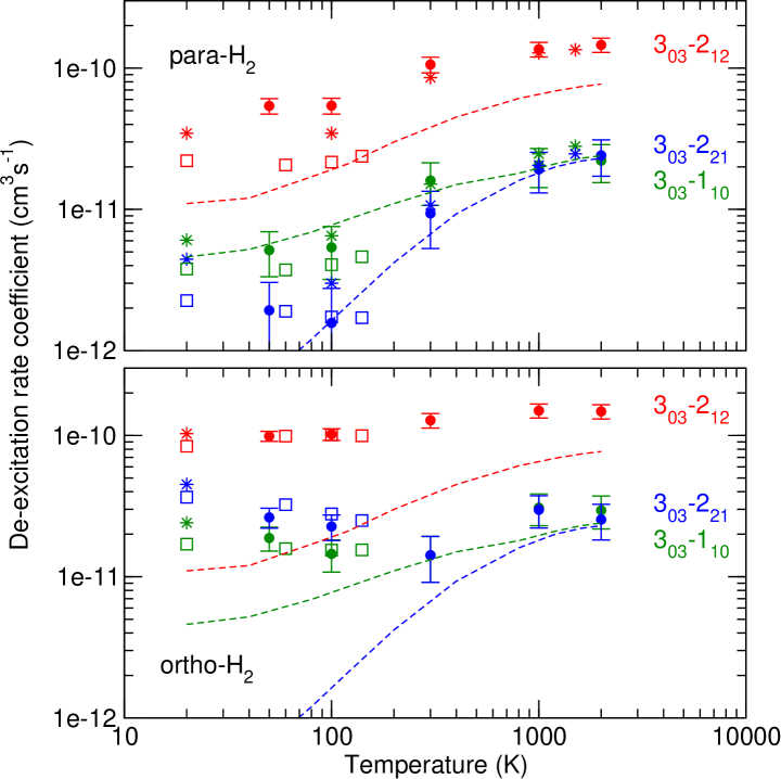
Figure 1: Rate coefficients, Eq. (2), for rotational de-excitation of the ortho-H₂O state $3_{03}$ as functions of temperature for para-H₂ (upper panel) and ortho-H₂ (lower panel). Squares denote quantum results by Phillips et al. (phillips96 (1996)); stars refer to the quantum calculations of Dubernet et al.; dashed lines denote quantum (scaled) results of Green et al. (green93 (1993)) for H₂O$-$He; circles with error bars (95% statistical confidence level) give the present QCT results. See text for details. Note that the transition $3_{03}\rightarrow 1_{01}$ is not plotted for clarity.

3.2 Accuracy and propensity rules

The above observations obviously hold for other initial levels and, from numerous comparisons, we estimate the QCT results to be accurate within a factor of 1$-$3 for the largest rates, i.e. those larger than a few 10^-12cm³s^-1, as observed in Faure et al. (faure06 (2006)). For smallest rates, errors larger than a factor of 3 can be encountered, illustrating the inability of classical mechanics to reproduce small probability events. As a result, rates less than $\sim$ 10^-12cm³s^-1, which correspond to very poor statistics (zero or less than $\sim$10 events over 10,000), were set to zero. This means that a significant number of transitions, the so-called classically forbidden or rare transitions, have null classical rates. Moreover, some transitions were found to have null rates at 100 K but significant rates at higher temperatures. Our strategy to tackle this problem was to retain transitions obeying the following two criteria: the rate must be i) larger than 10^-12cm³s^-1 at 300 K and above and ii) larger than 10^-11cm³s^-1 at 2000 K. If one of the two criteria is not fulfilled, then the transition is classified as a rare event and the corresponding (scaled) H₂O$-$He rate is adopted. It should be noted that these rare events correspond in most cases to transitions with $\Delta J>3$ which are not expected to play a dominant role in the radiative transfer equations (see Sect. 4). Moreover, despite the fact that no rigorous selection rules hold for molecule-molecule collisions, we actually observed the following propensity rules:

$$\Delta J=0,\pm 1;\hskip 14.22636pt\Delta K_{a}=0,\pm 1;\hskip 14.22636pt\Delta K_{c}=0,\pm 1,$$ (6)

which are consistent with the classical picture of a minimum reorientation of the angular momentum of a strongly asymmetric-top molecule. These rules are illustrated in Fig. 1 where the transition $3_{03}-2_{12}$ is indeed found to be strongly favoured.

3.3 Fitting procedure

For use in astrophysical modelling, the transition rates $R(J^{\prime}_{\alpha^{\prime}}\rightarrow J_{\alpha},T)$ must be evaluated on a sufficiently fine temperature grid. For this, the rates were first least-square fitted over 100$-$2000 K by the analytic form used by Faure et al. (faure04 (2004)):

$$\log_{10}R(J^{\prime}_{\alpha^{\prime}}\rightarrow J_{\alpha},T)=\sum_{n=0}^{N}a_{n}x^{n},$$ (7)

where $x=T^{-1/6}$. A typical fitting accuracy of a few percent was obtained. In the case of rare events with large error bars, the fitting method was also found to smooth the temperature dependence of the rates and thus remove irregularities caused by poor statistics. Note that $T=$50 K was investigated only for a few levels and was not retained in the fitting procedure. We then evaluated the fitted rates at the following grid temperature values: 100, 200, 400, 800, 1200, 1600 and 2000 K. From the H₂O$-$H₂ data of Phillips et al. (phillips96 (1996)), we observed the temperature dependence of de-excitation rates below 100 K to be very weak: de-excitation rates at 20 K are always within a factor of 2 of those at 100 K. This is clearly illustrated in Fig. 1. Below 100 K, a flat temperature dependence of the de-excitation rate was thus assumed, except for the lowest five para- and five ortho-H₂O levels for which the values at 20 K were taken from the quantum CC results of Dubernet et al. (dubernet06 (2006)). Such a flat low temperature dependence actually reflects the influence of the deep potential well of the H₂O$-$H₂ PES ($\sim$ 235 cm^-1) which supports large shape resonances, in contrast to H₂O$-$He ($\sim$ 35 cm^-1). Obviously, the above low temperature extrapolation procedure introduces errors but these are believed not to exceed a factor of 2$-$3 for the largest rates. The complete set of de-excitation rates among all 45 para- and ortho-H₂O levels between 20 and 2000 K are provided as online material and will be made available in the BASECOL database (http://www.obspm.fr/basecol/). Excitation rates can be obtained from the detailed balance relation, Eq. (5).

In order to assess quantitatively the impact of the new H₂O$-$H₂ collisional rates on water emission, detailed radiative transfer studies adapted to various astronomical environments are required. In Sect. 4 below, this impact is investigated for a range of density and temperature conditions by neglecting all excitation mechanisms other than collisions. A first-order indicator is also provided by the impact of rates on critical densities. For a multi-level system, the critical density of a given partner (here para- or ortho-H₂) is usually defined, in the optically thin case, given that the density at which the sum of the collisional de-excitation rates of a given level is equal to the sum of the spontaneous radiative de-excitation rates:

$$n_{cr}(J_{\alpha},T)=\frac{\sum_{J^{\prime}_{\alpha^{\prime}}}A(J_{\alpha}\rightarrow J^{\prime}_{\alpha^{\prime}})}{\sum_{J^{\prime}_{\alpha^{\prime}}}R(J_{\alpha}\rightarrow J^{\prime}_{\alpha^{\prime}},T)}.$$ (8)

When the colliding partner has a density $n\gg n_{cr}$, collisions maintain rotational levels in LTE at the kinetic temperature while for densities $n\lesssim n_{cr}$, deviations from LTE including population inversions are expected. Eq. (8) was computed with the present collisional rates for para-H₂ and ortho-H₂ and with the scaled H₂O$-$He rates of Green et al. (green93 (1993)). Einstein coefficients were taken from the Jet Propulsion Laboratory catalogue. Results are presented in Table 1 for 6 representative water levels, namely the upper level of the 557 GHz transition ($1_{10}-1_{01}$) and the upper levels of maser transitions known to be collisionally pumped (Yates et al. yates97 (1997)): the 183 GHz line ($3_{13}-2_{20}$), the 380 GHz line ($4_{14}-3_{21}$), the 325 GHz line ($5_{15}-4_{22}$), the 22 GHz line ($6_{16}-5_{23}$) and the 321 GHz line ($10_{29}-9_{36}$). Note that maser transitions are expected to be quite sensitive to relatively small differences in collisional rates. As illustrated in Table 1, critical densities for H₂ are decreased with respect to the scaled He values by a typical factor of 2$-$5 at 100 K and by a factor of 1$-$3 at higher temperatures. These differences are still modest (with the exception of $10_{29}$) because collisional rates are summed over all possible downward transitions, thus averaging the impact of the new rates. Larger differences in the emission line fluxes are however expected as individual state-to-state collisional rates, in particular with ortho-H₂, can exceed the scaled He values by more than an order of magnitude. This is demonstrated in Sect. 4. We conclude that using the new H₂O$-$H₂ collisional rates, non-LTE effects including population inversions will be quenched at lower H₂ densities, especially in regions where the H₂ ortho/para ratio is large.

Table 1: Critical densities, in cm^-3, for (scaled) He, para-H₂ and ortho-H₂, as functions of temperature and for a set of representative H₂O levels. Powers of 10 are given in parentheses. See text for details.

$J_{K_{a}K_{c}}$	$T$(K)	He	p-H2	o-H2	He/p-H2	He/o-H2
$1_{10}$	100	1.3(08)	6.3(07)	3.0(07)	2.1	4.3
	300	5.7(07)	3.6(07)	2.5(07)	1.6	2.3
	1000	3.0(07)	2.3(07)	2.2(07)	1.3	1.4
$3_{13}$	100	3.2(09)	1.1(09)	7.0(08)	2.9	4.6
	300	1.6(09)	7.7(08)	5.6(08)	2.1	2.9
	1000	8.4(08)	5.1(08)	4.5(08)	1.6	1.9
$4_{14}$	100	6.6(09)	2.5(09)	1.4(09)	2.6	4.7
	300	3.2(09)	1.5(09)	1.1(09)	2.1	2.9
	1000	1.5(09)	9.3(08)	8.2(08)	1.6	1.8
$5_{15}$	100	1.2(10)	4.8(09)	2.6(09)	2.5	4.6
	300	5.8(09)	2.9(09)	1.9(09)	2.0	3.1
	1000	2.5(09)	1.6(09)	1.4(09)	1.6	1.8
$6_{16}$	100	2.3(10)	8.6(09)	4.2(09)	2.7	5.5
	300	1.0(10)	4.9(09)	3.1(09)	2.0	3.2
	1000	4.1(09)	2.5(09)	2.1(09)	1.6	2.0
$10_{29}$	100	2.0(11)	4.0(10)	9.8(09)	5.0	20.4
	300	6.9(10)	1.9(10)	8.1(09)	3.6	8.5
	1000	2.0(10)	8.5(09)	6.3(09)	2.4	3.2

4 Modelling of water emission

In this section we explore, by means of a LVG code, the impact of the new computed collisional coefficients on the theoretical predictions of water line emission. The code is adapted from the one described in Ceccarelli et al. (ceccarelli02 (2002)). It refers to a semi-infinite isodense and isothermal slab (plane-parallel geometry). The code solves self-consistently the statistical level populations and the radiative transfer equations under the approximation of the escape probability, assuming a gradient in the velocity field (Capriotti capriotti65 (1965)). We consider the first 45 levels of both ortho- and para-H₂O separately. The computed line spectrum depends on a few basic parameters: the density of the colliders (H₂), the temperature of the emitting gas, the water column density and the maximum gas velocity. To have a relatively exhaustive study, we explored a large parameter space. We varied the H₂ density between 10⁴ and 10¹⁰ cm^-3; the kinetic temperature between 20 and 2000 K; the water column density between 10¹⁰ and 10¹⁵cm^-2, keeping the velocity equal to 1 km/s. Note that the velocity only enters in the line opacity, coupled with the H₂O column density. In the present study we considered specifically the case of optically thin lines (the low H₂O column density case), and the case where the lines are optically thick (the high H₂O column density case). In both cases, depending on the gas density, the collisional coefficients may play a major role in the predicted flux. Indeed, even in the case of strongly optically thick lines, the lines could be “effectively optically thin” if the levels are very sub-thermally populated, as is often the case for water lines. Finally, since the scope of this study is to understand the impact of the newly computed collisional coefficients in the line predictions, compared to the old ones, we did not consider the pumping of the levels by infrared and submillimetre radiation, which would unnecessarily complicate the problem.

We compared the results of the LVG computations with three sets of collisional data: the scaled H₂O-He rates of Green et al. (green93 (1993)) between 20 and 2000 K, the H₂O$-$H₂ rates of Phillips et al. (phillips96 (1996)) between 20 and 140 K and the present H₂O$-$H₂ classical rates beween 20 and 2000 K. The results of this comparison are reported in Fig. 2, where we show the line flux ratios for ortho-H₂O at representative densities and temperatures. Collision rates with ortho-H₂ only are considered to simplify the interpretation. The H₂O column density is fixed at 10¹⁵ cm^-2. It can be observed that LVG fluxes based on the classical rates are increased up to a factor of 10 with respect to LVG fluxes based on the scaled H₂O$-$He rates of Green et al. (green93 (1993)). Even larger differences were observed at lower temperatures. Second, LVG fluxes based on the classical rates are very similar to those based on the rates of Phillips et al. (phillips96 (1996)), with flux ratios close to 1. These findings clearly reflect the differences in collision rates, such as those illustrated in Fig. 1. They also show that differences in rates are not amplified within the radiative transfer equations. In particular, it is worth noting that the typical increase of fluxes at 1000 K is less than a factor of 2 at the investigated densities. Similar results were obtained with para-H₂, especially above 300 K where differences between para- and ortho-H₂ rates are minor. We note, however, that below 100 K, the classical para-H₂ rates are not necessarily more accurate than the scaled H₂O$-$He rates. Third, we observe that the flux ratios rise steeply with increasing upper energies. This is expected since the critical densities are larger for higher levels and, therefore, the impact of collision rates, i.e. non-LTE effects, becomes more pronounced. Finally, when the temperature increases, the impact of collision rates is reduced, partly because the low lying levels become thermalized and partly because the differences in rates decrease. It should be noted, however, that at densities higher than 10⁸cm^-3, large flux ratios ($\sim$ 10) were still observed at 1000 K for high lying levels.

We also tested the influence of the scaled H₂O$-$He rates employed as substitutes for H₂ rates in the case of classically-forbidden transitions. These rates, which generally correspond to $\Delta J>3$ and are lower than 10^-12 cm³s^-1, were found to play a minor role, especially at low temperatures ($T\leq$300 K). This suggests that the radiative transfer equations are above all sensitive to the largest rates. These findings however merit further investigation.

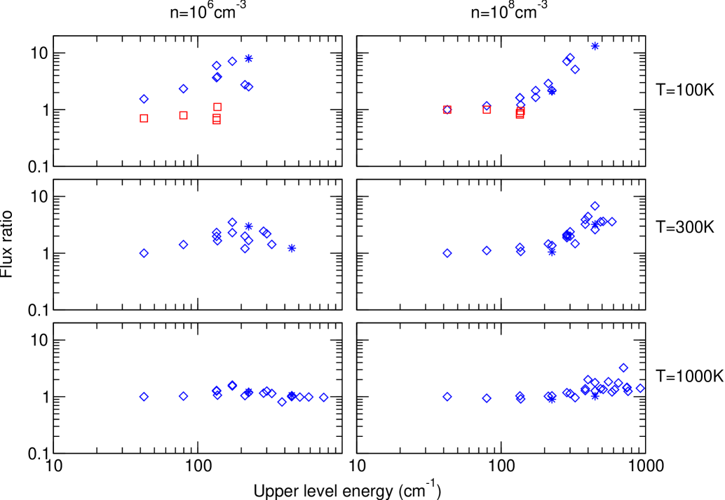
Figure 2: Emission line flux ratios from LVG modelling as functions of the upper energy levels of ortho-H₂O for representative densities and temperatures. Three differents sets of collision rates were employed (see text for details). The H₂O column density is fixed at 10¹⁵ cm^-2. Squares denote the ratios between LVG fluxes based on the classical rates and LVG fluxes based on the H₂O$-$H₂ rates of Phillips et al. (phillips96 (1996)). Diamonds and stars give the ratio between LVG fluxes based on the classical rates and LVG fluxes based on the scaled H₂O$-$He rate of Green et al. (green93 (1993)). Diamonds correspond to transitions whose fluxes are larger than 1% of the total flux; stars correspond to the radio transitions at 22 and 380 GHz.

5 Conclusions

We have computed classical rate coefficients for rotational de-excitation among the lowest 45 para and 45 ortho rotational levels of H₂O colliding with both para and ortho-H₂ in the temperature range 20$-$2000 K. Trajectories were run on a recent high-accuracy H₂O$-$H₂ PES using a canonical Monte-Carlo sampling. H₂ molecules were assumed to be rotationally thermalized at the kinetic temperature. By comparison with quantum calculations available for low lying levels, classical rates were found to be accurate within a factor of 1$-$3 for the dominant transitions, i.e. those with rates larger than a few 10^-12cm³s^-1. Large differences with the scaled H₂O$-$He rates of Green et al. (green93 (1993)) were observed and emission line fluxes were shown to be increased by up to a factor of 10. The present classical rates should therefore be adopted in any detailed population model of water in warm and hot environments.

It should be noted, however, that quantum CC calculations are currently in progress (Dubernet and co-workers) and quantum rates will ultimately replace the classical rates. It will thus be possible in future studies to further test the sensitivity of water emission to uncertainties in the collision rates and to identify, for example, physical regimes where classical rates are of sufficient accuracy. We also stress that the QCT method is currently the only practical approach to investigate very high rotational angular momenta. For example, water in supergiant stars has been observed through levels with rotational quantum number $J$ up to 23 (e.g. Jennings & Sada jennings98 (1998)). In order to assess non-LTE effects in such environments, classical calculations might provide precious information. Finally, we note that the first excited vibrational level of water lies only 2300 K above the ground state and it has been detected in several sources (e.g. Menten et al. menten06 (2006)). Rate coefficients for the total vibrational relaxation of H₂O by H₂ molecules have been computed by Faure et al. (2005a ) and some “$J$-resolved” cross sections can be found in Faure et al. (2005b ). Rovibrational state-to-state rates are however unknown and will be considered in future works.

- (1) Balakrishnan, N., Yan, M., & Dalgarno, A. 2002, ApJ, 568, 443
- (2) Bergin, E. A., & Snell, R. L. 2002, ApJ, 581, L105
- (3) Capriotti, E. R. 1965, ApJ, 142, 1101
- (4) Ceccarelli, C., Hollenbach, D. J., & Tielens, A. G. G. M. 1996, ApJ, 471, 400
- (5) Ceccarelli, C., et al. 2002, A&A, 383, 603
- (6) Cecchi-Pestellini, C., Bodo, E., Balakrishnan, N., & Dalgarno, A. 2002, ApJ, 571, 1015
- (7) Cernicharo, J., Thum, C., Hein, H., John, D., Garcia, P., & Mattioco, F. 1990, A&A, 231, L15
- (8) Cernicharo, J., Pardo, J. R., González-Alfonso, E., Serabyn, E., Phillips, T. G., Benford, D. J., & Mehringer, D. 1999, ApJ, 520, L131
- (9) Cernicharo, J., & Crovisier, J. 2005, Space Science Reviews, 119, 29
- (10) Cernicharo, J., Pardo, J. R., & Weiss, A. 2006, ApJ, 646, L49
- (11) Cheung, A. C., Rank, D. M., Townes, C. H., Thornton, D. D., & Welch, W. J. 1969, Nature, 221, 626
- (12) Doty, S. D., & Neufeld, D. A. 1997, ApJ, 489, 122
- (13) Dubernet, M.-L., & Grosjean, A. 2002, A&A, 390, 793
- (14) Dubernet, M.-L., Daniel, F., Grosjean A., et al. 2006, A&A, 460, 323
- (15) Dutta, J. M., Jones, C. R., Goyette, T. M., & de Lucia, F. C. 1993, Icarus, 102, 232
- (16) Faure, A., Gorfinkiel, J. D., & Tennyson, J. 2004, MNRAS, 347, 323
- (17) Faure, A., & Wiesenfeld, L. 2004, J. Chem. Phys., 121, 6771
- (18) Faure, A., Valiron, P., Wernli, M., Wiesenfeld, L., Rist, C., Noga, J., & Tennyson, J. 2005a, J. Chem. Phys., 122, 1102
- (19) Faure, A., Wiesenfeld, L., Wernli, M., & Valiron, P. 2005b, J. Chem. Phys., 123, 4309
- (20) Faure, A., Wiesenfeld, L., Wernli, M., & Valiron, P. 2006, J. Chem. Phys., 124, 214310
- (21) Flower, D. R., Roueff, E., & Zeippen, C. J. 1998, J. Phys. B: At. Mol. Opt. Phys., 31, 1105
- (22) Gilijamse, J. J., Hoekstra, S., van de Meerakker, S. Y. T., Groenenboom, G. C., Meijer, G., Science, 313, 1617
- (23) Goddi, C., Moscadelli, L., Sanna, A., Cesaroni, R., & Minier, V. 2007, A&A, 461, 1027
- (24) Green, S., Maluendes, S., & McLean, A. D. 1993, ApJS, 85, 181
- (25) Grosjean, A., Dubernet, M.-L., & Ceccarelli, C. 2003, A&A, 408, 1197
- (26) Hjalmarson, Å., Frisk, U., Olberg, M., et al. 2003, A&A, 402, L39
- (27) Jennings, D. E., & Sada, P. V. 1998, Science, 279, 844
- (28) Kondratko, P. T., Greenhill, L. J., & Moran, J. M. 2006, ApJ, 652, 136
- (29) Lefloch, B., Cernicharo, J., Cabrit, S., Noriega-Crespo, A., Moro-Martín, A., & Cesarsky, D. 2003, ApJ, 590, L41
- (30) Mandy, M. E., & Pogrebnya, S. K. 2004, J. Chem. Phys., 120, 5585
- (31) Melnick, G. J., & Bergin, E. A. 2005, Advances in Space Research, 36, 1027
- (32) Menten, K. M., Philipp, S. D., Güsten, R., Alcolea, J., Polehampton, E. T., & Brünken, S. 2006, A&A, 454, L107
- (33) Neufeld, D. A., & Melnick, G. J. 1991, ApJ, 368, 215
- (34) Neufeld, D. A., Melnick, G J., Sonnentrucker, P., et al. 2006, ApJ, 649, 816
- (35) Phillips, T. R., Maluendes, S., McLean, A. D., & Green, S. 1994, J. Chem. Phys., 101, 5824
- (36) Phillips, T. R., Maluendes, S., & Green, S. 1996, ApJS, 107, 467
- (37) Poelman, D. R., & Spaans, M. 2005, A&A, 440, 559
- (38) Poelman, D. R., Spaans, M., & Tielens, A. G. G. M. 2007, A&A, 464, 1023
- (39) Wernli, M., Wiesenfeld, L., Faure, A., & Valiron, P. 2007, A&A, 464, 1147
- (40) Wolniewicz, L., Simbotin, I., & Dalgarno, A. 1998, ApJS, 115, 293
- (41) Yates, J. A., Field, D., & Gray, M. D. 1997, MNRAS, 285, 303