Brownian motion in a non-homogeneous force field and photonic force microscope

Abstract

The Photonic Force Microscope (PFM) is an opto-mechanical technique based on an optical trap that can be assumed to probe forces in microscopic systems. This technique has been used to measure forces in the range of pico- and femto-Newton, assessing the mechanical properties of biomolecules as well as of other microscopic systems. For a correct use of the PFM, the force field to measure has to be invariable (homogeneous) on the scale of the Brownian motion of the trapped probe. This condition implicates that the force field must be conservative, excluding the possibility of a rotational component. However, there are cases where these assumptions are not fulfilled Here, we show how to improve the PFM technique in order to be able to deal with these cases. We introduce the theory of this enhanced PFM and we propose a concrete analysis workflow to reconstruct the force field from the experimental time-series of the probe position. Furthermore, we experimentally verify some particularly important cases, namely the case of a conservative or rotational force-field.

I Introduction

A focused optical beam - an optical tweezers - permits one to manipulate a wide range of particles - including atoms, molecules, DNA fragments, living biological cells, and organelles within them - with applications to many areas - such as molecular biophysics, genetic manipulation, micro-assembly, and micro-machines Ashkin (1970); Ashkin et al. (1986); Neuman and Block (2004). One of the most exciting applications has been the possibility to investigate and engineer the mechanical properties of microscopic systems - using, for example, optical traps as force transducers for mechanical measurements in biological systems Ashkin et al. (1990); Block et al. (1990); Svoboda et al. (1993); Kuo and Sheetz (1993); Finer et al. (1994).

In the early 90s various kinds of scanning probe microscopy were already established. The Scanning Tunneling Microscope (STM) Binnig et al. (1982) permits one to resolve at the atomic level crystallographic structures Binnig et al. (1983) and organic molecules Smith et al. (1990). The Atomic Force Microscope (AFM) Binnig et al. (1986) has been successfully employed to study biological and nano-fabricated structures, overcoming the diffraction limit of optical microscopes. Furthermore, they developed from pure imaging tools into more general manipulation and measuring tools on the level of single atoms or molecules. However, all these techniques required a macroscopic mechanical device to guide the probe.

A new kind of scanning force microscope using an optically trapped dielectric microsphere as a probe was proposed in Ghislain and Webb (1993); Ghislain et al. (1994). This technique was later called Photonic Force Microscope (PFM) Florin et al. (1997). In a typical setup, the probe is held in an optical trap, where it performs random movements due to its thermal energy. The analysis of this thermal motion provides information about the local forces acting on the probe. The three-dimensional probe position can be recorded through different techniques which detect its forward or backward scattered light. The most commonly used are a quadrant photodiode, a position sensing detector, or a high-speed video-camera Neuman and Block (2004). The PFM provides the capability of measuring forces in the range from femto- to pico-Newton. These values are well below those achieved with techniques based on micro-fabricated mechanical cantilevers, such as AFM Weisenhorn et al. (1989).

For small displacements of the probe from the center of an optical trap, the restoring force is proportional to the displacement. Hence, an optical trap acts on the probe like a Hookeian spring with a fixed stiffness, which can be characterized with various methods Visscher et al. (1996); Neuman and Block (2004). The correlation or power spectrum method, in particular, is considered the most reliable Visscher et al. (1996), allowing one to determine the trap stiffness by applying Boltzmann statistics to the position fluctuations of the probe, relying only on the knowledge of the temperature and the viscosity of the surrounding medium Ghislain and Webb (1993); Ghislain et al. (1994); Florin et al. (1997); Rohrbach and Stelzer (2002); Berg-Sørensen and Flyvbjerg (2004).

Assuming a very low Reynolds number regime Purcell (1977); Happel and Brenner (1983), the Brownian motion of the probe in the optical trap is described by a set of Langevin equations:

$$\gamma\mathbf{\dot{r}}(t)+\mathbf{K}\mathbf{r}(t)=\sqrt{2D}\gamma\mathbf{h}(t),$$ (1)

where $\mathbf{r}(t)=[x(t),y(t),z(t)]$ is the probe position, $\gamma=6\pi R\eta$ is its friction coefficient, $R$ is the probe radius, $\eta$ is the medium viscosity, $\mathbf{K}$ is the restoring force matrix, $\sqrt{2D}\gamma\mathbf{h}(t)=\sqrt{2D}\gamma[h_{x}(t),h_{y}(t),h_{z}(t)]$ is a vector of independent white Gaussian random processes describing the Brownian forces, $D=k_{B}T/\gamma$ is the diffusion coefficient, $T$ is the absolute temperature, and $k_{B}$ is the Boltzmann constant. The orientation of the coordinate system can be chosen in such a way that the restoring force is independent in the three directions, i.e. $\mathbf{K}=\mathrm{diag}(k_{x},k_{y},k_{x})$. In this reference frame the stochastic differential equations (1) are separated and without loss of generality the treatment can be restricted to the $x$-projection of the system.

The autocorrelation function (ACF) of the solution to equations (1) in each direction reads

$$<x(t)x(t+\Delta t)>=D\frac{\gamma}{k_{x}}e^{-k_{x}|\Delta t|/\gamma},$$ (2)

where $k_{x}$ is the trap stiffness. Experimentally the trap stiffness is found by fitting the theoretical ACF (2) to the one obtained from the measurements. Using the Wiener-Khintchine theorem, the power spectral density (PSD) can now be calculated as the Fourier transform of the ACF:

$$P_{x}(f)=\frac{D}{2\pi^{2}\left(f^{2}+f_{c}^{2}\right)},$$ (3)

where $f_{c}=k_{x}/2\pi\gamma$ is the corner frequency.

A constant and homogeneous external force $f_{ext,x}$ acting on the probe produces a shift in its equilibrium position in the trap. The value of the force can be obtained as:

$$f_{ext,x}=k_{x}<x(t)>,$$ (4)

where $<x(t)>$ is the probe mean displacement from the previous equilibrium position.

The PFM has been applied to measure forces in the range of femto- to pico-Newton in many different fields with exciting applications, for example, in biophysics, thermodynamics of small systems, and colloidal physics Ashkin et al. (1990); Block et al. (1990); Svoboda et al. (1993); Kuo and Sheetz (1993); Finer et al. (1994); Prälle et al. (1998); Menta et al. (1999); Prälle et al. (2000); Smith et al. (2001); Lang et al. (2002); Smith et al. (2003); Rohrbach (2005); Volpe et al. (2006a, b)

For a correct use of the PFM, the force field to measure has to be invariable (homogeneous) on the scale of the Brownian motion of the trapped probe, i.e. in a range of $10$s to $100$s of nanometers depending on the trapping stiffness. This condition implicates that the force field must be conservative, excluding the possibility of a rotational component. However, there are cases where these assumptions are not fulfilled as it is illustrated in Fig. 1. The field can vary in the nanometer scale, for example, in the presence of a radiation force field produced by a surface plasmon polariton Volpe et al. (2006b). It can also be non-conservative in the presence of a rotational force (torque). These effects appear, for example, considering the radiation forces exerted on a dielectric particle by a patterned optical near-field landscape at an interface decorated with resonant gold nanostructures Quidant et al. (2005) (Fig. 1(a)); the nanoscale trapping that can be achieved near a laser-illuminated tip Novotny et al. (1997) (Fig. 1(b)); the optical forces produced by a beam which carries orbital angular momentum Volpe and Petrov (2006) (Fig. 1(c)); or in the presence of fluid flows Volpe et al. (2007).

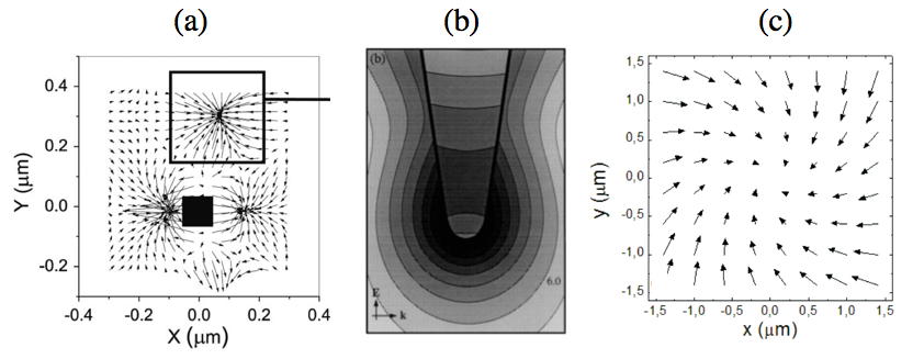
Figure 1: (Color online) Examples of physical systems that produce forces fields that can not be correctly probed with a classical PFM because they vary on the scale of the Brownian motion of the trapped probe, i.e. in a range of $10$s to $100$s of nanometers : (a) forces produced by a surface plasmon polariton in the presence of a patterned surface on a $50\,nm$ radius dielectric particle (reproduced from Quidant et al. (2005)); (b) electromagnetic near-field of a $10\,nm$ wide gold tip in water illuminated by a $810\,nm$ monochromatic light beam (reproduced from Novotny et al. (1997)); and (c) vector force field acting on a $500\,nm$ radius dielectric particle in the focal plane of a highly focused Laguerre-Gaussian beam (reproduced from Volpe and Petrov (2006)).

In this article, we show how to improve the PFM technique in order to be able to deal with these cases. We introduce the theory of this enhanced PFM (section II). Based on this theoretical understanding, in section III we propose a concrete analysis workflow to reconstruct the force field from the experimental time-series of the probe position. Finally, in section IV we present experimental results for some particularly important cases, namely the case of a conservative or rotational force-field.

II Theory

In the presence of an external force field $\mathbf{f_{ext}}(\mathbf{r}(t))$, equation (1) can be written in the form:

$$\gamma\mathbf{\dot{r}}(t)=\mathbf{f}(\mathbf{r}(t))+\sqrt{2D}\gamma\mathbf{h}(t),$$ (5)

where the total force acting on the probe $\mathbf{f}\left(\mathbf{r}(t)\right)=\mathbf{f_{ext}}(\mathbf{r}(t))-\mathbf{K}\mathbf{r}(t)=\left[f_{x}(\mathbf{r}(t)),f_{y}(\mathbf{r}(t))\right]$ depends on the position of the probe itself, but does not vary over time. We reduce our analysis to a bidimensional system, because it is the most interesting from the applied point of view. However, our approach can be generalized to the tridimensional case.

The force $\mathbf{f}(\mathbf{r}(t))$ can be expanded in Taylor series up to the first order around an arbitrary point $\mathbf{\tilde{r}}$:

$$\mathbf{f}(\mathbf{r}(t))=\underbrace{\left[\begin{array}[]{c}f_{x}(\mathbf{\tilde{r}})\\ f_{y}(\mathbf{\tilde{r}})\\ \end{array}\right]}_{\mathbf{f_{\tilde{r}}}}+\underbrace{\left[\begin{array}[]{cc}\partial_{x}f_{x}(\mathbf{\tilde{r}})&\partial_{y}f_{x}(\mathbf{\tilde{r}})\\ \partial_{x}f_{y}(\mathbf{\tilde{r}})&\partial_{y}f_{y}(\mathbf{\tilde{r}})\\ \end{array}\right]}_{\mathbf{J_{\tilde{r}}}}\left(\mathbf{r}(t)-\mathbf{\tilde{r}}\right)+o\left(||\mathbf{r}-\mathbf{\tilde{r}}||\right),$$ (6)

where $\mathbf{f_{\tilde{r}}}$ and $\mathbf{J_{\tilde{r}}}$ are the zeroth-order expansion, i.e. the force field value at the point $\mathbf{\tilde{r}}$, and the Jacobian of the force field calculated in $\mathbf{\tilde{r}}$, respectively.

In a PFM the probe particle is optically trapped and, therefore, it diffuses due to Brownian motion in the total force field (the sum of the optical one and the one under investigation). If $\mathbf{f_{\tilde{r}}}\neq\mathbf{0}$, the probe experiences a shift in the direction of the force. After a time has elapsed, therefore, the particle settles down in a new equilibrium position of the total force field, such that $\mathbf{f_{\tilde{r}}}=\mathbf{0}$. As seen in the introduction, the measurement of this shift allows one to evaluate the homogeneous force acting on the probe in the standard PFM. Assuming, without loss of generality, $\mathbf{\tilde{r}}=\mathbf{0}$, the statistics of the Brownian motion in the surroundings of the equilibrium point can be analyzed in order to reconstruct the force field up to its first-order approximation.

II.1 Brownian motion near an equilibrium position

The first order approximation to equation (5) near a stable force field equilibrium point, $\mathbf{\tilde{r}}=\mathbf{0}$, is:

$$\mathbf{\dot{r}}(t)=\gamma^{-1}\mathbf{J_{0}}\mathbf{r}(t)+\sqrt{2D}\mathbf{h}(t),$$ (7)

where $\mathbf{r}(t)=\left[x(t),y(t)\right]$, $\mathbf{h}(t)=\left[h_{x}(t),h_{y}(t)\right]$, and $\mathbf{J_{0}}$ is the Jacobian calculated in the equilibrium point. According to the Helmholtz theorem, under reasonable regularity conditions any force field can be separated into its conservative (i.e. irrotational) and non-conservative (i.e. rotational or solenoidal) components. The two components can be immediately identified if the coordinate system is chosen such that $\partial_{y}f_{x}(\mathbf{0})=-\partial_{x}f_{y}(\mathbf{0})$. In this case, the Jacobian $\mathbf{J_{0}}$ normalized by the friction coefficient $\gamma$ reads:

$$\gamma^{-1}\mathbf{J_{0}}=\left[\begin{array}[]{cc}-\phi_{x}&\Omega\\ -\Omega&-\phi_{y}\\ \end{array}\right],$$ (8)

where $\phi_{x}=k_{x}/\gamma$ and $\phi_{y}=k_{y}/\gamma$, $k_{x}=-\partial_{x}f_{x}(\mathbf{\tilde{r}})$ and $k_{y}=-\partial_{y}f_{y}(\mathbf{\tilde{r}})$, and $\Omega=\gamma^{-1}\partial_{y}f_{x}(\mathbf{\tilde{r}})=-\gamma^{-1}\partial_{x}f_{y}(\mathbf{\tilde{r}})$. In (8) the rotational component, which is invariant under a coordinate rotation, is represented by the non-diagonal terms of the matrix: $\Omega$ is the value of the constant angular velocity of the probe rotation around the $z$ axis due to the presence of the rotational force field Volpe and Petrov (2006). The conservative component, instead, is represented by the diagonal terms of the Jacobian and is centrally symmetric with respect to the origin. Without loss of generality, we impose that $k_{x}>k_{y}$, i.e. $\phi_{x}>\phi_{y}$. This means that the stiffness of the trapping potential is higher along the $x$-axis.

The equilibrium point is stable if:

$$\left\{\begin{array}[]{*{20}l}\mathrm{Det}\left(\mathbf{J_{0}}\right)=\phi^{2}-\Delta\phi^{2}+\Omega^{2}\geq 0\\ \mathrm{Tr}\left(\mathbf{J_{0}}\right)=-2\phi\leq 0\\ \end{array}\right.,$$ (9)

where $\phi=(\phi_{x}+\phi_{y})/2$ and $\Delta\phi=(\phi_{x}-\phi_{y})/2$. The fundamental condition required to achieve stability is $\phi>0$. Assuming that this condition is satisfied, the behavior of the optically trapped probe can be explored as a function of the parameters $\Omega/\phi$ and $\Delta\phi/\phi$. The stability diagram is shown in Fig. 2. The standard PFM corresponds to $\Delta\phi=0$ and $\Omega=0$. When a rotational term is added, i.e. $\Omega\neq 0$ and $\Delta\phi=0$, the system remains stable Volpe and Petrov (2006). When there are no rotational contributions to the force field ($\Omega=0$) the equilibrium point becomes unstable as soon as $\Delta\phi\geq\phi$. This implicates that $\phi_{y}<0$, and therefore the probe is not confined in the $y$-direction any more. In the presence of a rotational component ($\Omega\neq 0$) the stability region becomes larger; the equilibrium point now becomes unstable only for $\Delta\phi\geq\sqrt{\phi^{2}-\Omega^{2}}$.

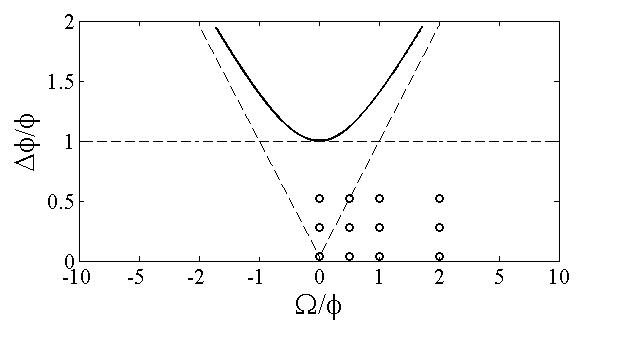
Figure 2: (Color online) Stability diagram. Assuming $\phi>0$, the stability of the system is shown as a function of the parameters $\Omega/\phi$ and $\Delta\phi/\phi$. The regions that satisfy the conditions described in equation (9). The continuos line delimits the stability region. The dashed lines represent the $\Delta\phi=|\Omega|$ and $\Delta\phi=\phi$. The dots represent the parameters that are further investigated in Fig. (3), (4) and (5).

Some examples of possible force fields are presented in Fig. 3.

When $\Omega=0$ the probe movement can be separated along two orthogonal directions. As the value of $\Delta\phi$ increases the probability density function (PDF) of the probe position becomes more and more elliptical, until for $\Delta\phi\geq\phi$ the particle is confined only along the $x$-direction and the confinement along the $y$-direction is lost.

If $\Delta\phi=0$, the increase in $\Omega$ induces a bending of the force field lines and the probe movement along the $x$- and $y$-directions are not independent any more. For values of $\Omega\geq\phi$, the rotational component of the force field becomes dominant over the conservative one. This is particularly clear when $\Delta\phi\neq 0$: the presence of a rotational component covers the asymmetry in the conservative one, since the probability density distribution assumes a more rotationally-symmetric shape.

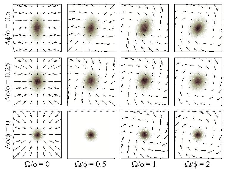
Figure 3: (Color online) The arrows show the force field vectors for various values of the parameters $\Delta\phi/\phi$ and $\Omega/\phi$. The shadowed areas show the probability distribution function (PDF) of the probe position in the corresponding force field.

II.2 Enhanced Photonic Force Microscope

As we already mentioned in the introduction, the most powerful analysis method is based on the study of the correlation functions - or, equivalently, the power spectral density - of the probe position time-series. In this subsection, we derive the correlation matrix first in the coordinate system considered in the previous subsection, where the conservative and rotational components are separated. We, then, derive the same matrix in a generic coordinate system and identify some functions that are independent on the choice of the coordinate system. For completeness, we will also present the power spectral density matrix.

II.2.1 Correlation Matrix

The correlation matrix of the probe motion near an equilibrium position can be calculated from the solutions of (7), whose eigenvalues are $\lambda_{1,2}=-\phi\pm\sqrt{\Delta\phi^{2}-\Omega^{2}}$ and whose eigenvectors are $\mathbf{v_{1,2}}=\left[\Omega,\Delta\phi\pm\sqrt{\Delta\phi^{2}-\Omega^{2}}\right]^{T}$.

Treating $\mathbf{h}(t)$ as a driving function, the solution of (7) is given by:

$$\mathbf{r}(t)=\sqrt{2D}\int_{-\infty}^{t}\mathbf{W}(t)\mathbf{W}^{-1}(s)\mathbf{h}(s)ds,$$ (10)

where

$$\mathbf{W}(t)=\left[\begin{array}[]{cc}\Omega&\Omega\\ \Delta\phi+\sqrt{\Delta\phi^{2}-\Omega^{2}}&\Delta\phi-\sqrt{\Delta\phi^{2}-\Omega^{2}}\\ \end{array}\right]\left[\begin{array}[]{cc}e^{\lambda_{1}t}&0\\ 0&e^{\lambda_{2}t}\\ \end{array}\right]$$ (11)

is the Wronskian of the system.

Since we are assuming $\mathbf{r}(t)$ to be a stationary stochastic process, the correlation matrix $\left<\mathbf{r}(t+\Delta t)\mathbf{r^{*}}\left(t\right)\right>$ can be obtained by taking the ensemble average $\left<\mathbf{r}(\Delta t)\mathbf{r^{*}}\left(0\right)\right>$:

$$\left<\mathbf{r}(\Delta t)\mathbf{r^{h}}\left(0\right)\right>=\left<2D\int_{-\infty}^{\Delta t}\mathbf{W}(\Delta t)\mathbf{W}^{-1}(t^{\prime})\mathbf{h}(t^{\prime})dt^{\prime}\int_{-\infty}^{0}\mathbf{h^{h}}(t^{\prime\prime})\mathbf{W}^{-1\mathbf{h}}(t^{\prime\prime})\mathbf{W^{h}}(0)dt^{\prime\prime}\right>,$$ (12)

where the superscript $h$ indicates the hermitian. Solving this system, we have

$$r_{xx}(\Delta t) = D\frac{e^{-\phi\left|\Delta t\right|}}{\phi}\left[\left(\frac{\Omega^{2}-\alpha^{2}\Delta\phi^{2}}{\Omega^{2}-\Delta\phi^{2}}-\alpha^{2}\frac{\Delta\phi}{\phi}\right)\mathcal{C}(\Delta t)-\alpha^{2}\frac{\Delta\phi}{\phi}\left(1-\frac{\Delta\phi}{\phi}\right)\mathcal{S}(|\Delta t|)\right],$$ (13)

$$r_{yy}(\Delta t) = D\frac{e^{-\phi\left|\Delta t\right|}}{\phi}\left[\left(\frac{\Omega^{2}-\alpha^{2}\Delta\phi^{2}}{\Omega^{2}-\Delta\phi^{2}}+\alpha^{2}\frac{\Delta\phi}{\phi}\right)\mathcal{C}(\Delta t)+\alpha^{2}\frac{\Delta\phi}{\phi}\left(1+\frac{\Delta\phi}{\phi}\right)\mathcal{S}(|\Delta t|)\right],$$ (14)

$$r_{xy}(\Delta t) = D\frac{e^{-\phi\left|\Delta t\right|}}{\phi}\frac{\Omega}{\phi}\left[+\mathcal{S}(\Delta t)+\alpha^{2}\frac{\Delta\phi}{\phi}\left(\mathcal{C}(\Delta t)+\mathcal{S}(|\Delta t|)\right)\right],$$ (15)

$$r_{yx}(\Delta t) = D\frac{e^{-\phi\left|\Delta t\right|}}{\phi}\frac{\Omega}{\phi}\left[-\mathcal{S}(\Delta t)+\alpha^{2}\frac{\Delta\phi}{\phi}\left(\mathcal{C}(\Delta t)+\mathcal{S}(|\Delta t|)\right)\right],$$ (16)

where

$$\alpha^{2}=\frac{\phi^{2}}{\phi^{2}+\left(\Omega^{2}-\Delta\phi^{2}\right)}$$ (17)

is a dimensionless positive parameter,

$$\mathcal{C}(t)=\left\{\begin{array}[]{cc}\cos\left(\sqrt{|\Delta\phi^{2}-\Omega^{2}|}t\right)&\Omega^{2}>\Delta\phi^{2}\\ 1&\Omega^{2}=\Delta\phi^{2}\\ \mathrm{cosh}\left(\sqrt{|\Delta\phi^{2}-\Omega^{2}|}t\right)&\Omega^{2}<\Delta\phi^{2}\\ \end{array}\right.$$ (18)

and

$$\mathcal{S}(t)=\left\{\begin{array}[]{cc}\phi\frac{\sin\left(\sqrt{|\Delta\phi^{2}-\Omega^{2}|}t\right)}{\sqrt{|\Delta\phi^{2}-\Omega^{2}|}}&\Omega^{2}>\Delta\phi^{2}\\ \phi t&\Omega^{2}=\Delta\phi^{2}\\ \phi\frac{\mathrm{sinh}\left(\sqrt{|\Delta\phi^{2}-\Omega^{2}|}t\right)}{\sqrt{|\Delta\phi^{2}-\Omega^{2}|}}&\Omega^{2}<\Delta\phi^{2}\\ \end{array}\right..$$ (19)

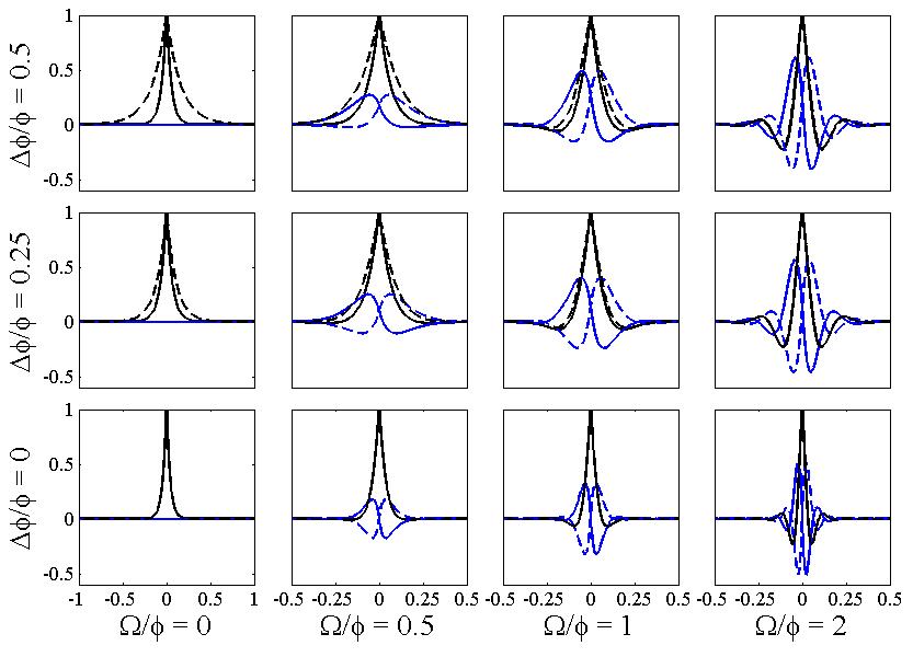
Figure 4: (Color online) Auto- and cross-correlation functions for various values of the parameters $\Delta\phi/\phi$ and $\psi/\phi$: $r_{xx}$ (black continuous line), $r_{yy}$ (black dotted line), $r_{xy}$ (blue continuous line), and $r_{yx}$ (blue dotted line).

In Fig. 4 these functions are plotted for different ratios of the force field conservative and rotational components. Some cases have already been studied experimentally. For the case $\Delta\phi=0$ Volpe and Petrov (2006), the ACFs and cross-correlation functions (CCFs) are $r_{xx}(\Delta t)=r_{yy}(\Delta t)=De^{-\phi|\Delta t|}\cos(\Omega\Delta t)/\phi$ and $r_{xy}(\Delta t)=-r_{yx}(\Delta t)=De^{-\phi|\Delta t|}\sin(\Omega\Delta t)/\phi$, respectively. As the rotational component becomes greater than the conservative one ($\Omega>\phi$), a first zero appears in the ACFs and CCFs and, as $\Omega$ increases even further, the number of oscillation grows. Eventually, for $\Omega\gg\phi$ the sinusoidal component becomes dominant. The conservative component manifests itself as an exponential decay of the magnitude of the ACFs and CCFs.

When $\Omega=0$, the movement of the probe along the $x$- and $y$-directions becomes independent. The ACFs behave as $r_{xx}(\Delta t)=De^{-\phi_{x}|\Delta t|}/\phi_{x}$ and $r_{yy}(\Delta t)=De^{-\phi_{y}|\Delta t|}/\phi_{y}$, while the CCFs are null, $r_{xy}(\Delta t)=r_{yx}(\Delta t)=0$. In Fig. 2 this case is represented by the line $\Omega=0$.

When both $\Omega$ and $\Delta\phi$ are zero, the ACFs are $r_{xx}(\Delta t)=r_{yy}(\Delta t)=De^{-\phi|\Delta t|}/\phi$, and the CCFs are null, $r_{xy}(\Delta t)=r_{yx}(\Delta t)=0$. The corresponding force field vectors point towards the center and are rotationally symmetric.

It is also interesting to consider the intermediate cases. In these cases the effective angular frequency that enter the expression is given by $\sqrt{|\Delta\phi|^{2}-\Omega^{2}}$. This shows that the difference in the stiffness coefficients along the $x$- and $y$-axes effectively influences the rotational term, if this is present. A limiting case is when $|\Omega|=\Delta\phi$. This case presents a kind of resonance between the rotational term and the stiffness difference. However, it is not a dramatic resonance, as it is shown by the corresponding force field (Fig. 3).

II.2.2 Correlation matrix in a generic coordinate system

The expression for the ACFs and CCFs (13) to (16) were obtained in a specific coordinate system, where the conservative and rotational component of the force field can be easily identified. However, typically the experimentally acquired time-series of the probe position required for the calculation of the ACFs and CCFs are given in a different coordinate system, rotated with respect to the one considered above. If a rotated coordinate system is introduced, such that:

$$\left[{\begin{array}[]{*{20}c}{x^{\prime}}\\ {y^{\prime}}\\ \end{array}}\right]=\left[{\begin{array}[]{*{20}c}{\cos\theta}&{-\sin\theta}\\ {\sin\theta}&{\cos\theta}\\ \end{array}}\right]\left[{\begin{array}[]{*{20}c}x\\ y\\ \end{array}}\right],$$ (20)

the correlation functions in the new system are obtained as linear combinations of (13)-(16):

$$r_{x^{\prime}x^{\prime}}(\Delta t) = \left(\cos{\theta}\right)^{2}r_{xx}(\Delta t)-\cos{\theta}\sin{\theta}r_{xy}(\Delta t)-\sin{\theta}\cos{\theta}r_{yx}(\Delta t)+\left(\sin{\theta}\right)^{2}r_{yy}(\Delta t),$$ (21)

$$r_{y^{\prime}y^{\prime}}(\Delta t) = \left(\sin{\theta}\right)^{2}r_{xx}(\Delta t)+\sin{\theta}\cos{\theta}r_{xy}(\Delta t)+\cos{\theta}\sin{\theta}r_{yx}(\Delta t)+\left(\cos{\theta}\right)^{2}r_{yy}(\Delta t),$$ (22)

$$r_{x^{\prime}y^{\prime}}(\Delta t) = \cos{\theta}\sin{\theta}r_{xx}(\Delta t)+\left(\cos{\theta}\right)^{2}r_{xy}(\Delta t)-\left(\sin{\theta}\right)^{2}r_{yx}(\Delta t)-\sin{\theta}\cos{\theta}r_{yy}(\Delta t),$$ (23)

$$r_{y^{\prime}x^{\prime}}(\Delta t) = \sin{\theta}\cos{\theta}r_{xx}(\Delta t)-\left(\sin{\theta}\right)^{2}r_{xy}(\Delta t)+\left(\cos{\theta}\right)^{2}r_{yx}(\Delta t)-\cos{\theta}\sin{\theta}r_{yy}(\Delta t),$$ (24)

which in general depend on $\theta$. However, it is remarkable that the difference of the two CCFs and the sum of the ACFs are invariant:

$$r_{x^{\prime}y^{\prime}}(\Delta t)-r_{y^{\prime}x^{\prime}}(\Delta t) = 2D\frac{e^{-\phi\left|\Delta t\right|}}{\phi}\frac{\Omega}{\phi}\mathcal{S}(\Delta t),$$ (25)

$$r_{x^{\prime}x^{\prime}}(\Delta t)+r_{y^{\prime}y^{\prime}}(\Delta t) = 2D\frac{e^{-\phi\left|\Delta t\right|}}{\phi}\left[\left(\frac{\Omega^{2}-\alpha^{2}\Delta\phi^{2}}{\Omega^{2}-\Delta\phi^{2}}\right)\mathcal{C}(\Delta t)+\alpha^{2}\frac{\Delta\phi^{2}}{\phi^{2}}\mathcal{S}(|\Delta t|)\right].$$ (26)

These functions are presented in Fig. 5. These functions are very similar to the ones presented in Fig. 4; however, the latter depend on the coordinate system choice.

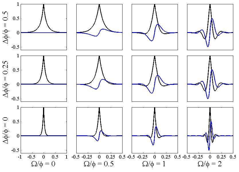
Figure 5: (Color online) Functions independent from choice of the reference system for various values of the parameters $\Delta\phi/\phi$ and $\Omega/\phi$: $r_{x^{\prime}x^{\prime}}+r_{y^{\prime}y^{\prime}}$ (black line) and $r_{x^{\prime}y^{\prime}}-r_{y^{\prime}x^{\prime}}$ (blue line).

Other two combinations of (21)-(24), which are also useful for the analysis of the experimental data, namely the sum of the CCFs and the difference of the ACFs, depend on the choice of the reference frame:

$$r_{x^{\prime}y^{\prime}}(\Delta t)+r_{y^{\prime}x^{\prime}}(\Delta t) = 2D\frac{e^{-\phi\left|\Delta t\right|}}{\phi}\alpha^{2}\frac{\Delta\phi}{\phi}\left(\mathcal{C}(\Delta t)+\mathcal{S}(|\Delta t|)\right)\left(\frac{\Omega}{\phi}\cos{(2\theta)}-\sin{(2\theta)}\right),$$ (27)

$$r_{x^{\prime}x^{\prime}}(\Delta t)-r_{y^{\prime}y^{\prime}}(\Delta t) = -2D\frac{e^{-\phi\left|\Delta t\right|}}{\phi}\alpha^{2}\frac{\Delta\phi}{\phi}\left(\mathcal{C}(\Delta t)+\mathcal{S}(|\Delta t|)\right)\left(\frac{\Omega}{\phi}\sin{(2\theta)}+\cos{(2\theta)}\right).$$ (28)

Their plots are shown in Fig. 6. In particular, when they are evaluated for $\Delta t=0$, they deliver information on the orientation of the coordinate system.

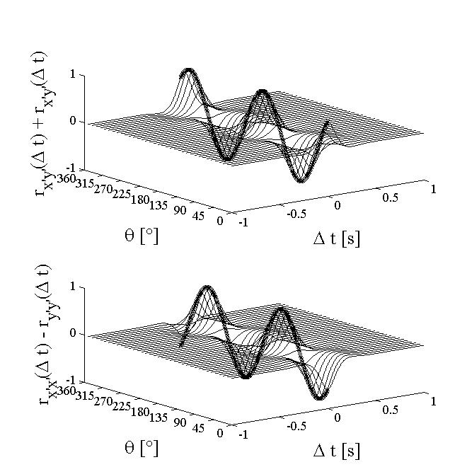
Figure 6: (Color online) Functions which depend on the orientation of the coordinate system for various values of the parameters as a function of the angle with respect to the coordinate system chosen in the section II: (a) $r_{x^{\prime}x^{\prime}}-r_{y^{\prime}y^{\prime}}$ and (b) $r_{x^{\prime}y^{\prime}}+r_{y^{\prime}x^{\prime}}$. The thicker lines show the values for $\Delta t=0$.

II.2.3 Power Spectral Density Matrix

In the frequency domain the equation (5) is given by:

$$i2\pi f\mathbf{R}(f)=\mathbf{J_{0}}\mathbf{R}(f)+\sqrt{2D}\mathbf{H}(f),$$ (29)

and its solution is $\mathbf{R}(f)=\sqrt{2D}\left(i2\pi f\mathbf{I_{2}}-\mathbf{J_{0}}\right)^{-1}\mathbf{H}(f)$, where $\mathbf{I_{2}}$ is the 2D unit matrix, and the corresponding PSD matrix:

$$\mathbf{P}(f)=\mathbf{R}\cdot\mathbf{R^{h}}=\frac{2D}{|\left(\phi_{x}+i2\pi f\right)\left(\phi_{y}+i2\pi f\right)+\psi^{2}|^{2}}\left[\begin{array}[]{cc}\phi_{y}^{2}+4\pi^{2}f^{2}+\psi^{2}&\psi\left[\phi_{x}-\phi_{y}-i4\pi f\right]\\ \psi\left[\phi_{x}-\phi_{y}+i4\pi f\right]&\phi_{x}^{2}+4\pi^{2}f^{2}+\psi^{2}\\ \end{array}\right]$$ (30)

where the property $\mathbf{H}(f)\cdot\mathbf{H^{h}}(f)=\mathbf{I_{2}}$ has been used. We notice that the PSD matrix could have been obtained as Fourier-transfor of the correlation matrix (Wiener-Khintchine theorem).

III Experimental Considerations

In this section we propose a concrete analysis workflow to reconstruct the force field from the experimental time-series of the probe position.

Experimentally the probe position time-series is the only available information to reconstruct the force field. Typically these data are obtained in an arbitrary coordinate system. These time-series need to be statistically analyzed in order to reconstruct all the parameters of the force field, i.e. $\phi$, $\Delta\phi$, and $\Omega$, and the orientation of the coordinate system. The detailed procedure to retrieve all this information from the experimental data is presented in this section.

Let us suppose to have the probe position time-series in a generic coordinate system $\mathbf{r^{\prime}}(t)=\left[x^{\prime}(t),y^{\prime}(t)\right]$, First, we evaluate the parameters $\phi$, $\Delta\phi$, and $\Omega$. Then, we transform the coordinate system to the one presented in the section II, where the conservative and rotational components are separated. Finally, we reconstruct the total force field. Eventually, the trapping force field may be subtracted to retrieve the external force field under investigation.

In order to illustrate this method we proceed to analyze some numerically simulated data. The main steps of this analysis are presented in Fig. 7. In Fig. 7(a) the PDF is shown for the case of a probe in a force field with the following parameters: $\phi=37.1\,s^{-1}$, $\Delta\phi=9.3\,s^{-1}$ (corresponding to $k_{x}=43.25\,pN/\mu m$ and $k_{y}=26.25\,pN/\mu m$), $\Omega=0$, and $\theta=30^{\circ}$. The PDF is ellipsoidal due to the difference of the stiffness along two orthogonal directions. In Fig. 7(b) the PDF for a force field with the same $\phi$ and $\Delta\phi$ but with $\Omega=37.1\,s^{-1}$ is presented. The presence of the rotational component in the force field produces two main effects. First, the PDF is more rotationally-symmetric and its main axes undergo a further rotation. Secondly, as we show below, the CCF is not null (Fig. 7(d)).

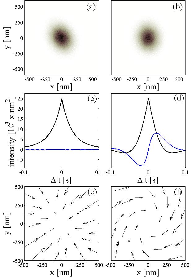
Figure 7: (Color online) (a-b) Probability density function for a Brownian particle under the influence of the force-field shown in the inset; in (a) the force-field is purely conservative, while in (b) it has a rotational component. (c-d) Invariant function, $r_{x^{\prime}x^{\prime}}+r_{y^{\prime}y^{\prime}}$ (black line) and $r_{x^{\prime}y^{\prime}}-r_{y^{\prime}x^{\prime}}$ (blue line). (e-f) Force fields obtained form the numerically simulated data.

III.1 Evaluation of the parameters $\phi$, $\Delta\phi$, and $\Omega$

In order to evaluate the parameters of the force field, $\phi$, $\Delta\phi$, and $\Omega$, we calculate the correlation matrix in the coordinate system where the experiments have been done,

$$\left\langle{{\bf r^{\prime}}(\Delta t){\bf r^{\prime}}^{\bf h}(0)}\right\rangle=\left({\begin{array}[]{*{20}c}r_{x^{\prime}x^{\prime}}(\Delta t)&r_{x^{\prime}y^{\prime}}(\Delta t)\\ r_{y^{\prime}x^{\prime}}(\Delta t)&r_{y^{\prime}y^{\prime}}(\Delta t)\\ \end{array}}\right).$$ (31)

Then we calculate the CCF difference (25), $r_{x^{\prime}y^{\prime}}(\Delta t)-r_{y^{\prime}x^{\prime}}(\Delta t)$. As we showed in section II, this function is invariant with respect to the choice of the reference system, and it is different form zero only if $\Omega\neq 0$. The results are shown in Fig. 7(c) and 7(d) for the cases of the data shown in Fig. 7(a) and 7(b) respectively. The three aforementioned parameters can be found by fitting the experimental data to the theoretical shape of this function. In particular, the exponential decay of the function is related to the $\phi$ parameter; the period of the superimposed oscillations is related to the effective angular frequency $\sqrt{|\Delta\phi^{2}-\Omega^{2}|}$; and the sign of the slope in $\Delta t=0$ gives the sign of $\Omega$.

When $\Omega=0$, the CCF difference (25) is null (Fig. 7(c)), it can not be used to find the two remaining parameters. For $\Omega=0$, the other invariant function, the ACF sum (equation (26)), is given by

$$r_{x^{\prime}x^{\prime}}(\Delta t)+r_{y^{\prime}y^{\prime}}(\Delta t)=2D\frac{e^{-\phi\left|\Delta t\right|}}{\phi}\left[\frac{\phi^{2}}{\phi^{2}-\Delta\phi^{2}}\mathcal{C}(\Delta t)+\frac{\Delta\phi^{2}}{\phi^{2}-\Delta\phi^{2}}\mathcal{S}(\Delta t)\right].$$ (32)

$\phi$ and $\Delta\phi$ can be evaluated by fitting the data to (32). The function (26) can be used for the fitting of the three parameters but can not give information on the sign of $\Omega$, which must be retrieved from the sign of the slope at $\Delta t=0$ of the CCF difference.

III.2 Coordinate system transformation

Although the values of the parameters $\phi$, $\Delta\phi$, and $\Omega$ are now known, the directions of the force vectors are still missing. In order to retrieve the orientation of the experimental coordinate system, we now use the orientation dependent functions (27) and (28). The best choice is to evaluate the two functions for $\Delta t=0$, because the signal-to-noise ratio is highest at this point:

$$\left\{{\begin{array}[]{*{20}c}{r_{x^{\prime}y^{\prime}}(0)+r_{y^{\prime}x^{\prime}}(0)=2D\frac{\alpha^{2}}{\phi}\frac{\Delta\phi}{\phi}\left(\frac{\Omega}{\phi}\cos{(2\theta)}-\sin{(2\theta)}\right)}\\ {r_{x^{\prime}x^{\prime}}(0)-r_{y^{\prime}y^{\prime}}(0)=-2D\frac{\alpha^{2}}{\phi}\frac{\Delta\phi}{\phi}\left(\frac{\Omega}{\phi}\sin{(2\theta)}+\cos{(2\theta)}\right)}\\ \end{array}}\right..$$ (33)

The solution of this system delivers the value of the rotation angle $\theta$. If $\Delta\phi=0$, (33) is undetermined as a consequence of the PDF radial symmetry. In this case any orientation can be used. If $\Omega=0$, the orientation of the coordinate system coincide with the axis of the PDF ellipsoid and, although (33) can still be used, the Principal Component Analysis (PCA) algorithm is a convenient means to determine their directions.

III.3 Reconstruction of the force field

Now everything is ready to reconstruct the unknown force field acting on the probe around the equilibrium position in an area comparable with the mean square displacement of the probe. From the values of $\phi$ and $\Delta\phi$, the conservative forces acting on the probe result ${\bf f}_{c}(x,y)=-\left({k_{x}x{\bf e}_{x}+k_{y}y{\bf e}_{y}}\right)$ and, from the values of $\Omega$, the rotational force is ${\bf f}_{r}(x,y)=\Omega\left({y{\bf e}_{x}-x{\bf e}_{y}}\right)$. The total force field is

$${\bf f}(x,y)={\bf f}_{c}(x,y)+{\bf f}_{r}(x,y)=\left(-k_{x}x+\Omega y\right){\bf e}_{x}-\left(k_{y}y+\Omega x\right){\bf e}_{y}x$$ (34)

in the rotated coordinate system. Now the rotation (20) can be used in order to have the force field in the experimental coordinate system. The unknown component can be easily reconstructed by subtraction of the know ones, such as the optical field.

IV Experimental results

For an experimental verification of our conclusions, we analyze the Brownian motion of an optically trapped polystyrene sphere in the presence of an external force field generated by a fluid flow Volpe et al. (2007). A schematic of the setup is presented in Fig. 8.

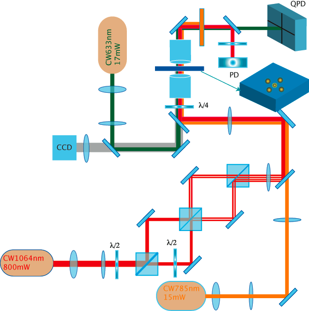
Figure 8: (Color online) Experimental setup.

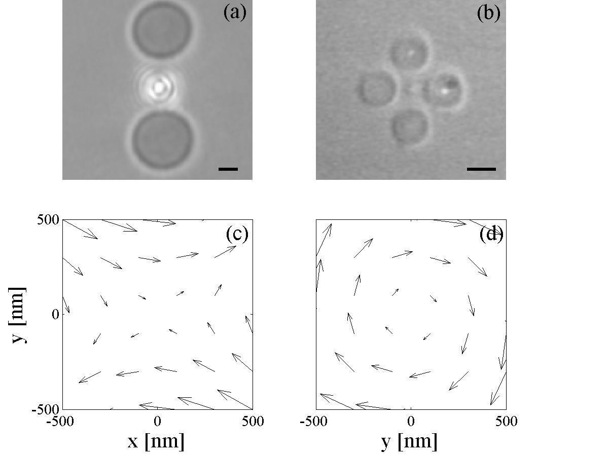
Figure 9: (Color online) Experimental configuration with two (a) and four (b) spinning beads and respective force fields (c) and (d).

An optical trap is generated by a CW $633\,nm$ beam at the focal plane of a $100\times$ $1.3NA$ objective lens inside a chamber. The chamber is prepared using two cover slips separated by a $50\,\mu m$ spacer and filled with a solution containing polystyrene spheres (radius $R=0.5\,\mu m$). The forward scattered light from the trapped sphere is collimated by a $50\times$ objective onto a quadrant photodiode (QPD). The trap force constant can be adjusted by changing the intensity of the laser beam.

The fluid flow that produces the external force field was generated using solid spheres made of a birefringent material (Calcium Vaterite Crystals (CVC) spheres, radius $R=1.5\pm 0.2\mu m$ Bishop et al. (2004)), which can be made spin due to the transfer of orbital angular momentum of light. They are all-optically controlled, i.e. their position can be controlled by an optical trap and their spinning state can be controlled through the polarization state of the light. In our experimental realization up to four CVC spheres were optically trapped in water and put into rotation using four steerable $1064\,nm$ beams from a Nd:YAG laser with controllable polarization - to control the direction of the rotation - and power - to control the rotation rate.

IV.1 Conservative force field

In order to produce a conservative force field, two CVC were placed as shown in Fig. 9(a), which should theoretically produce the force field presented in Fig. 9(c).

In Fig. 10(a), the invariant functions, $r_{x^{\prime}x^{\prime}}+r_{y^{\prime}y^{\prime}}$ (black line) and $r_{x^{\prime}y^{\prime}}-r_{y^{\prime}x^{\prime}}$ (blue line), and respective fitting to the theoretical shapes are presented. The CCF difference tells us that $\Omega=0$ in this case, while the fitting to the ACF sum tells us the values of $\phi=18\,s^{-1}$ and $\Delta\phi=6\,s^{-1}$. The value of the rotation of the coordinate system in this case is $32^{\circ}$.

The total force field can now be recontructed: $k_{x}=225\,fN/\mu m$ and $k_{y}=112\,fN/\mu m$. This force field is presented in Fig. 10(b). We can now retrieve the hydrodynamic force field by subtracting the optical force field ($k_{opt}=185\,fN/\mu m$ approximatively constant in all directions), that can be measured in absence of rotation of the spinning beads.

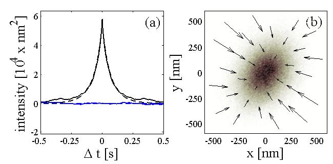
Figure 10: (Color online) (a) Invariant functions, $r_{x^{\prime}x^{\prime}}+r_{y^{\prime}y^{\prime}}$ (black line) and $r_{x^{\prime}y^{\prime}}-r_{y^{\prime}x^{\prime}}$ (blue line), and respective fitting to the theoretical shape (dotted lines). (b) Experimental probability density function and estimated force field.

IV.2 Rotational force field

In order to produce a rotational force field, four CVC were placed as shown in Fig. 9(b), which should theoretically produce the force field presented in Fig. 9(d).

In Fig. 11(a), the invariant functions, $r_{x^{\prime}x^{\prime}}+r_{y^{\prime}y^{\prime}}$ (black line) and $r_{x^{\prime}y^{\prime}}-r_{y^{\prime}x^{\prime}}$ (blue line), and respective fitting to the theoretical shapes are presented. Now the CCF difference is not null any more and tehrefore it can be used to fit the three parameters: $\phi=11\,s^{-1}$, $\Delta\phi\approx 0$, and $\Omega=5\,rads^{-1}$. We can notice that the ACF sum can be used for this purpose as well; however, we have to remark that using the latter the sign of $\Omega$ stays undetermined. The small value of $\Delta\phi$ implicates that the rotation of the coordinate system is not crucial.

The total force field can now be recontructed: $k_{x}\approx k_{y}=100\,fN/\mu m$. This force field is presented in Fig. 11(b). We can now retrieve the hydrodynamic force field by subtracting the optical force field ($k_{opt}=78\,fN/\mu m$ approximatively constant in all directions), that can be measured in absence of rotation of the spinning beads.

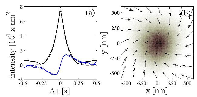
Figure 11: (Color online) (a) Invariant functions, $r_{x^{\prime}x^{\prime}}+r_{y^{\prime}y^{\prime}}$ (black line) and $r_{x^{\prime}y^{\prime}}-r_{y^{\prime}x^{\prime}}$ (blue line), and respective fitting to the theoretical shape (dotted lines). (b) ) Experimental probability density function and estimated fore field.

V Conclusion

We have shown how the PFM can be applied to the detection of locally non-homogeneous force fields. This has been achieved by analyzing the ACFs and CCFs of the probe position time-series. We believe that this technique can gain new insights into micro- and molecular-scale phenomena. In these cases the presence of the Brownian motion is intrinsic and has can not be disregarded. Therefore this technique permits one to take advantage to the Brownian fluctuations of the probe in order to explore the force field present in its surroundings.

One of the most remarkable advantages of the technique we propose is that it can be implemented in all existing PFM-setups and even on data acquired in the past. Indeed, it does not require changes to be made in the physical setup, but only to analyze the data in a deeper way.