Flat Energy histogram version for Interacting Growth Walk

Abstract

Interacting Growth Walks is a recently proposed stochastic model for studying the coil-globule transition of linear polymers. We propose a flat energy histogram version for Interacting Growth Walk. We demonstrate the algorithm on two dimensional square and triangular lattices by calculating the density of energy states of Interacting Self Avoiding Walks.

Monte Carlo methods have emerged as a powerful and reliable tool for simulating several complex phenomena in statistical physics, see, e.g., landau ; KPN . Conventional Monte Carlo methods landau are found inefficient for simulating models with complicated energy landscapes, such as spin glasses or protein folding. There are many variants of the sampling techniques proposed to address these issues, see, e.g., parallel tempering paral . Several efforts have focussed on algorithms that aim to produce a nearly uniform distribution in one or more of the macroscopic observables, such as energy or number of particles, within a predetermined range, which often fall in the class of so-called flat histogram methods, see below.

Flat histogram techniques permit enhanced flexibility in sampling of energy space in that the system is given a greater probability for escaping low-lying energy minima as compared to traditional Boltzmann sampling. Multicanonical, transition matrix, and Wang- Landau algorithms landau1 are some examples. These approaches have been used extensively to study liquid crystals, protein folding, and polymer phase behaviour braz ; binder . This letter focusses on a flat energy histogram method to study the coil-globule transition of linear polymers.

Long polymer chains in a good solvent have been studied extensively over the last five decades. Substantial progress has been made on elucidation of macroscopic properties as well as scaling behaviour of an isolated polymer chain from lattice models, see e.g. vander . Mostly, these have been based on self avoiding walks, as they incorporate in their basic definition excluded volume effect.

Self Avoiding Walk (SAW) is a random walk in which a walk cannot visit a site more than once vander . In order to study the thermodynamic properties of SAW, one needs to assign energy to each conformation. A standard way of doing this for a lattice SAW is to assign an energy $\epsilon$ to each nonbonded nearest neighbor (nbNN) contact in the walk. So, a conformation with $m$ such contacts has energy $E=m\ \epsilon$. A SAW with energy assigned in this fashion is called an interacting self-avoiding walk(ISAW) vander . For the study of coil to globule transition of linear homopolymers, one can set $\epsilon=-1$ without loss of generality.

Many conventional SAW Monte Carlo algorithms pivot and their variants have been formulated for obtaining equilibrium properties of ISAW. In a recent paper Rechnitzer and Rensberg rech define a random variable called ’atmosphere’. It is the number of possible ways a self avoiding walk of length $n$ on a lattice can proceed to create a walk of length $n+1$. They showed that from the statistics of atmosphere one can estimate the connective constant and entropic exponent rech .

More recently Prellberg and Krawczyk interpreted the atmosphere as proportional to Rosenbluth and Rosenbluth (RR) weight RR in a stochastic growth algorithm flatperm . They show that RR walks in conjuction with the so-called ’dynamic’ pruning and enrichment perm provides a flat histogram Monte Carlo algorithm.

In a recent work pon2 , we have generalized the notion of atmosphere to other possible growth algorithms; we have shown that the average of atmosphere taken over ensembles of different stochastic growth algorithms give an estimate of the density of states of ISAW. In particular we have considered the Interacting Growth Walk (IGW) igw1 ; igw2 . When RR walks are kineticaly interpreted one gets Kinetic Growth Walk (KGW) kgw . In the same way when the PERM-B walks of Grassberger Grassberger-PERM-B are kinetically intepreted one gets Interacting Growth Walk igw1 .

In IGW the first step from the origin to nearest neighbour site is taken randomly and independently with probability $1/z$ where $z$ is the coordination number of the lattice. Subsequent steps are taken with local IGW probability $p_{j}$. Let us say that at $j^{th}$ step, $a_{j}$ unvisited nearest neighbour sites are available for the walk to proceed. The probability for choosing the $\alpha^{th}_{j}$ unvisited site is given by

$$p_{j}(\alpha_{j})=\frac{exp[\beta_{G}m_{nbNN}(\alpha_{j})]}{\sum_{\alpha_{j}=1}^{a_{j}}exp[\beta_{G}m_{nbNN}(\alpha_{j})]},$$ (1)

where $\beta_{G}$ is a model growth parameter; $m_{{\rm nbNN}}(\alpha_{j})$ is the number of nonbonded nearest neighbour contacts the walk would make if it were to step onto the $\alpha_{j}^{th}$ nearest neighbour site. If the number of unvisited nearest neighbour sites is zero at any stage, the walk is terminated (trapping); the entire walk is then discared and one starts all over again. For a given $\beta_{G}$, the probability of generating an $N$ step IGW is given by,

$$P_{N}=B(\beta_{G})\times\prod_{j=1}^{N}p_{j},$$ (2)

where $B(\beta_{G})$ is the normalization constant. The atmosphere for this $N$ step IGW is given by pon2 ,

$$A_{N} = \prod_{j=1}^{N}\frac{1}{p_{j}}.$$ (3)

For $\beta_{G}=0$, every unvisited nearest neighbour site is chosen with equal probability. Therefore IGW reduces to KGW kgw in the limit $\beta_{G}\to 0$ igw2 . For large $\beta_{G}>0$ the walks generated by the IGW are extremely compact. If $\beta_{G}<0$, the walk would prefer to step onto that site that leads to lesser number of contacts. Hence for large negative $\beta_{G}$ the walk generated by the IGW would be mostly extended as compared to those with $\beta_{G}=0$.

In this letter we propose a flat histogram Interacting Growth Walk. We show the atmosphere, when averaged over the flat histogram IGW ensemble, provides a powerful technique for estimating the density of states (DOS).

In flat histogram IGW, the growth parameter $\beta_{G}$ is taken as a random variable. The fluctuations of $\beta_{G}$ are so adjusted that it ensures uniform accumulation of $N$-step ISAWs in all the energy bins. In other words if $H(E)$ denotes the energy histogram of $N$-step ISAWs, then the random variation of $\beta_{G}$ from one step to the next in a walk and from one walk to the other in the ensemble, leads to a flat $H(E)$.

The energy of an $n$ step ISAW having $m$ contacts is given by $E_{n}=m\epsilon$. Let $m_{n}^{max}$ denote the maximum number of contacts possible in an $n$ step ISAW. Then the number of energy levels is $m_{n}^{max}+1$. These are indexed by $k=1,2,...(m_{n}^{max}+1)$. Thus $E_{n}$ can take values from zero to $m_{n}^{max}\epsilon$ and the correspoding energy histogram is represented by $H_{n}(k)$. We also define an array $\mathcal{G}_{n}(k)$, called atmosphere sum, described below.

In an $N$-step flat histogram IGW algorithm, $H_{n}(k)$ and $\mathcal{G}_{n}(k)$ are initially set zero for all $n(1\leq n\leq N)$ and $\forall\ k$. In a simulation run, if a walk at $n^{th}$ step has an energy $E$ which corresponds to index $k$, then $H_{n}(k)$ and $\mathcal{G}_{n}(k)$ incremented as,

$$H_{n}(k) = H_{n}(k)+1$$

$$\mathcal{G}_{n}(k) = \mathcal{G}_{n}(k)+A_{n},$$ (4)

where

$$A_{n} = \prod_{j=1}^{n}\frac{1}{p_{j}}$$ (5)

is the atmosphere pon2 for $n^{th}$step for that run and $p_{j}$ is the probability for $j^{th}$ step which depends upon the value of $\beta_{G}$ at that step. The implementation of the above algorithm proceeds as follows.

The first step $(n=1)$ of the walk starts from the origin with probability $1/z$, where $z$ is the coordination number of the chosen lattice. For $n=1,\ m_{1}^{max}=0$ and $A_{1}=z$; the energy histogram and atmosphere sum corresponding to the first step is incremented as $H_{1}(1)=H_{1}(1)+1$ and $\mathcal{G}_{1}(1)=\mathcal{G}_{1}(1)+z$. All subsequent steps ($j\geq 2$) are taken with probability $p_{j}$ given by Eq. (1). The value of $\beta_{G}$ for each $n(>1)$ is chosen depending upon the difference between $H_{n}(\eta+1)$ and $H_{n}(\eta)$, where $\eta=1,2,...(m_{n-1}^{max}+1)$. In order to span all energy levels the following procedure is adopted in this algorithm.

Let

$$\Delta = \left\{H_{n}(\eta+1)-H_{n}(\eta)\right\}\ \xi$$ (6)

$$\mathfrak{B} = min\left\{\ |\Delta|\ ,\ \beta_{G}^{max}\ \right\},$$ (7)

where $\xi$ is a random number that takes values uniformly between zero to one and $\beta_{G}^{max}$ is the maximum value assigned to avoid overflow/underflow problem. The value of $\beta_{G}$ is chosen as

$$\beta_{G}=\left\{\begin{array}[]{lll}+\mathfrak{B}&if&\Delta<0\\ -\mathfrak{B}&if&\Delta>0\\ \ \mathrm{0}&if&\Delta=0.\\ \end{array}\right.$$ (11)

During each growth ste,p $\beta_{G}$ takes a value between $-\beta_{G}^{max}$ and $\beta_{G}^{max}$. The corresponding $H_{n}$ and $\mathcal{G}_{n}$ are incremented as in Eq.(Flat Energy histogram version for Interacting Growth Walk). The walk is continued till it gets trapped or $n$ reaches $N$. The above procedure is repeated for several number of Monte Carlo attempts M. Estimator for density of states, $g(E)$, corresponding to the energy levels $k=1,2,..(m_{n}^{max}+1)$ of ISAW $\forall\ n\leq N$ is then given by

$$g^{est}_{n}(k)=\frac{\mathcal{G}_{n}(k)}{M}.$$ (12)

From the density of states we can calculate the canonical partition function $Z=\sum_{E}g(E)\exp(-\beta E)$ where $\beta=1/k_{B}T$. From the partition function one can calculate any thermodynamic property.

A general property of IGW is that with increase of $\beta_{G}$ longer walks can be generated with increasing probabilities igw2 . In otherwords, attrition is less when $\beta_{G}$ is large. In fact on a two dimensional square lattice, there is no attrition when $\beta_{G}\to\infty$ igw2 ; igwhoney . In the context of flat histogram IGW the parameter that control fluctuation of $\beta_{G}$ is $\beta_{G}^{max}$. Hence if $\beta_{G}^{max}$ is large, flat histogram IGW can generate longer walks spanning uniformly all the energy levels.

The flat histogram IGW described above was implemented on a two dimensional square lattice. Figure 1 depicts the energy histogram for $N=199$ and $299$ for flat histogram IGW with $\beta_{G}^{max}=10$. We find that proper choice of $\beta_{G}^{max}$ would lead better statistics of density of states. Thus in our simulation on a square lattice we have chosen $\beta_{G}^{max}=1.0$ and $N\leq 300$. The reduced histogram $h_{n}(k)=H_{n}(k)/max\{H_{n}(k)\}\ \forall k$ for $n=25$ to $300$ (insteps of $25$) is shown in Figure 2. The histograms are flat. The estimated density of states for shorter walk length compared with exact enumeration results is shown in Figure 3. The simulation results match well with the exact results. The statistical error of each Monte Carlo data point does not exceed $\pm 1\%$. The plot of estimated density of states versus energy for walk length $n=10$ to $120$ (insteps of $10$) is shown in Figure 4. These results were obtained over $10^{8}$ Monte Carlo attempts.

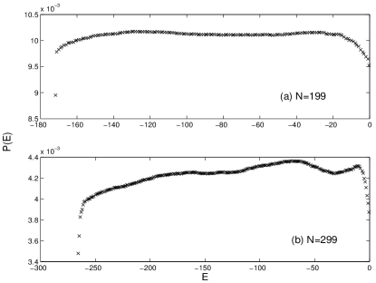
Figure 1: Flat histogram IGW with $\beta_{G}^{max}=10$: Energy distribution for $N=199$ and $299$. The energy distributions are reasonably flat.

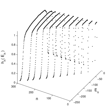
Figure 2: Plot of reduced histogram $h_{n}(E_{n})$ versus energy $E_{n}$ and length $n=25$ to $300$ (insteps of $25$: right to left) for ISAW. These have been obtained from flat histogram IGW on a square lattice with $\beta_{G}^{max}=1.0$ and $M=10^{8}$ attempts.

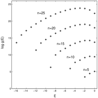
Figure 3: Semilog plot of estimated density of states $g^{est}_{n}(E_{n})$ versus energy $E_{n}$ and length $n=5$ to $25$ (insteps of $5$) for ISAW on a square lattices obtained from flat histogram IGW with $\beta_{G}^{max}=1.0$; $M=10^{8}$. The Monte Carlo results ($\star$) matches very well with exact (+) density of states. ( Monte Carlo errors are very small; maximum of error does not exeed one percent and are within the symbol size on the scale).

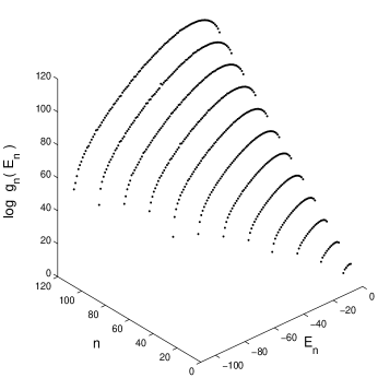
Figure 4: Semilog plot of estimated density of states $g^{est}_{n}(E_{n})$ versus energy $E_{n}$ and length $n=10$ to $120$ (insteps of $10$: right to left) for ISAW on a square lattice obtained from flat histogram IGW with $\beta_{G}^{max}=1.0$; $M=10^{8}$.

We have calculated fluctuations of energy, $\sigma^{2}(E)=\langle E^{2}\rangle-\langle E\rangle^{2}$ as a function of $\beta$. This is shown in Figure 5. The value of $\beta\sim(1/1.54)\sim 0.649$ vander at which phase transition is expected to occur is marked by vertical line. The fluctuations are maximum at the transition temperature.

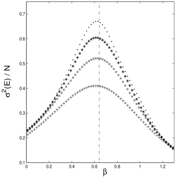
Figure 5: Energy fluctuation per walk length $\sigma^{2}(E)/N$ versus inverse temperature $\beta$ for ISAW on a square lattice for $N=30(+),50(\times),70(\ast)$ and $90(\cdot)$. The vertical lines denote the expected transition temperature in the thermodynamic limit $N\to\infty$.

The ”art” of making flat histogram IGW to estimate exactly the DOS of ISAW for various lattices and various dimensions are based to a large extent on a suitable choice of $\beta_{G}^{max}$. Flat histogram IGW simulation on triangular lattice also were carried out with $\beta_{G}^{max}=0.8$. The plot of reduced histogram and density of state are shown in Figure 6 .

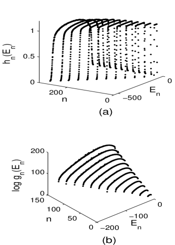
Figure 6: Flat histogram IGW on a triangular lattice. (a) Plot of reduced histogram (b) Semilog plot of $g_{n}^{est}(E_{n})$ vs $E_{n}$ for various $n$; $\beta_{G}^{max}=0.8$; $M=10^{8}$.

In conclusion we have presented a flat energy histogram method to study Interacting Self Avoiding Walks. This method is based on IGW algorithm. Monte Carlo simulation of flat histogram IGW for longer self avoiding walks with large $\beta_{G}^{max}$ one can obtain resonably flat energy histogram. By optimizing $\beta_{G}^{max}$ one can estimate density of states with good statics. We have carried out flat histogram IGW simulation of self avoiding walks on square and triangular lattices and presents results on DOS of ISAW and flat energy histogram.

- (1) D.P. Landau and K. Binder, A Guide to Monte Carlo Simulations in Statistical Physics (Cambridge University Press, Cambridge, 2000).
- (2) K.P.N. Murthy, Monte Carlo methods in Statistical Physics (University Press, India, 2004).
- (3) A. Schug, T. Herges, A. Verma and W. Wenzel, J. Phys.: Condens. Matter 17, S1641-S1650 (2005).
- (4) D.P. Landau, S. H. Tsai and M. Exler, Am. J. Phys. 72, 1294 (2004).
- (5) A. G. Cunha Netto, C. J. Silva, A. A. Caparica and R. Dickman, Brazilian Journal of Physics, 36, 619 (2006).
- (6) W. Paul, T. Strauch, F. Rampf, and K. Binder, Phys. Rev. E ( Rapid commun.), 75, 060801 (2007).
- (7) C. Vanderzande, Lattice Models of Polymers (Cambridge University Press, 1998)
- (8) Tom Kennedy, J. Stat. Phys. 106, 407 (2002)
- (9) A. Rechnitzer and E.J. Janse van Rensburg J. Phys. A: Math. Gen. 35, L605 (2002).
- (10) M.N. Rosenbluth and A.W. Rosenbluth, J.Chem Phys. 23, 356 (1955)
- (11) T. Prellberg and J. Krawczyk, Phys. Rev. Lett. 92, 120602 (2004).
- (12) P. Grassberger, Phys.Rev.E. 56, 3682 (1997).
- (13) M.Ponmurugan, V. Sridhar, S.L. Narasimhan and K.P.N. Murthy, ”A flat histogram method based on Interacting Self Avoiding Walks”, International Conference on Materials for Advanced Technology (ICMAT 2007), July 2007, Singapore.
- (14) S.L. Narasimhan, P.S.R. Krishna, K.P.N. Murthy and M. Ramanadham, Phys. Rev. E ( Rapid commun.), 65, 010801 (2002).
- (15) S.L.Narasimhan, P.S.R. Krishna, A.K. Rajarajan and K.P.N. Murthy, Phys. Rev. E 67, 011802 (2003).
- (16) I. Majid, N. Jan, A. Coniglio and H.E. Stanley, Phys. Rev. Lett. 52, 1257 (1984).
- (17) H.P. Hsu, V. Mehra, W. Nadler, and P. Grassberger, Phys. Rev. E 68, 021113 (2003).
- (18) S. L. Narasimhan, V. Sridhar and K. P. N. Murthy, Physica A 320, 1 (2003)