Precise determination of orbital parameters in system with slowly drifting phases: application to the case of XTE J1807–294

Abstract

We describe a timing technique that allows to obtain precise orbital parameters of an accreting millisecond pulsar in those cases in which intrinsic variations of the phase delays (caused e.g. by proper variation of the spin frequency) with characteristic timescale longer than the orbital period do not allow to fit the orbital parameters over a long observation (tens of days). We show under which conditions this method can be applied and show the results obtained applying this method to the 2003 outburst observed by RXTE of the accreting millisecond pulsar XTE J1807–294 which shows in its phase delays a non-negligible erratic behavior. We refined the orbital parameters of XTE J1807–294 using all the 90 days in which the pulsation is strongly detected and the method applicable. In this way we obtain the orbital parameters of the source with a precision more than one order of magnitude better than the previous available orbital solution, a precision obtained to date, on accreting millisecond pulsars, only for SAX J1808.4–3658 analyzing several outbursts spanning over seven years and with a much better statistics.

1 Introduction

Low Mass X-ray Binaries (LMXB) are binary systems in which one of the two stars is a neutron star (NS) with low magnetic field ($<10^{9}\mathrm{Gauss}$) which accretes matter from a low-mass ($<1\,M_{\odot}$) companion star. According to the so-called recycling scenario (see for a review Bhatta_91) millisecond radio pulsars originate from LMXBs, where the accretion torques and the relatively weak magnetic fields are able to spin up the NSs up to millisecond periods. When the companion star stops transferring matter to the NS, the NS can switch on as millisecond radio pulsar.

A striking confirmation of this scenario was the discovery in 1998 of millisecond X-ray pulsars in transient LMXBs. The first LMXB observed to show coherent pulsations at a frequency of $\sim 400$ Hz was the well studied SAX J1808.4–3658 (Wijnands_98; Chakra_98). Due to the weak magnetic field of these sources, the chance to see a pulsed emission from a LMXB is quite low. However, to date 8 LMXBs were discovered to be accreting millisecond pulsars (Wijnands_05), and all of them are in transient systems. They spend most of the time in a quiescent state, with very low luminosities (of the order of $10^{31}-10^{32}$ ergs/s) and rarely we go into an X-ray outburst with luminosities in the range $10^{36}-10^{37}$ ergs/s. Indeed, of all these sources only SAX J1808.4–3658, which shows more or less regular outbursts every two years, has been observed in outburst more than once with RXTE. All the other sources have shown just one outburst in the RXTE era.

This fact makes the study of the timing properties of these sources even more difficult, given that the duration of the observations is not a matter of choice, but is conditioned by the duration of the outbursts which, in turns, puts a constrain on the precision of the parameters that we can derive. And this is also the reason why we have to obtain all the information and the precision of the parameters we need just using the available data. In the case of accreting millisecond pulsars, among the parameters of interest there are, of course, the timing parameters, that are the orbital parameters and the spin parameters. The orbital parameters can give us important information on the binary system, its evolution, and even on the nature (e.g. degenerate or not) of the companion star. Also, a precise orbital solution will be important for a precise determination of the spin parameters, the spin period evolution and the accretion torques acting onto the NS.

As already mentioned above, the knowledge with the maximum possible precision of the orbital parameters is of fundamental importance in itself and for a successive study of the spin and the spin variations. The study of the frequency Doppler shift due to orbital motion of a millisecond pulsar in a binary system is the first step to obtain an estimate of the set of orbital parameters. To refine this estimate the next step is the study of the pulse phase shifts in order to obtain differential corrections to the orbital parameters and therefore a finer orbital solution. However, in some cases, not all the data in which the coherent X-ray pulsations are visible can be easily used to obtain the differential corrections. The pulse phase shifts are frequently affected by intrinsic long-term variations and/or fluctuations (probably caused by the accretion torques) which are superimposed to the modulation due to the orbital motion of the source, making the fit of the residual sinusoidal modulation much more complicated. Clear examples of these complex behaviors of the pulse phase shifts in accreting millisecond pulsars can be found in Burderi_06, who analyze SAX J1808.4–3658 and find a big jump in the pulse phase shifts of the fundamental harmonic of the pulse, and in Papitto_07, who analyze XTE J1814–338 finding a modulation of the pulse phase shifts, anti-correlated to the X-ray flux, superposed on a general spin-down trend.

Of course, the presence of non negligible long-term variations of the pulse phase shifts with time, make it very difficult to fit a long dataset with differential correction as reported in Eq.3 in order to obtain a precise estimate of the orbital parameters using all the available time-span. Using the classical technique it is then necessary, in order to decouple the orbital modulation from the proper fluctuations of the pulse phases, to take into account the latter in some way. This is often impossible to obtain by fitting with a simple model, due to the observed complex behaviors and/or our poor knowledge of the physics of the accretion torques. In such cases we are forced to fit differential corrections of the orbital parameters on restricted time intervals, in which the proper fluctuations or variations of the phase shifts can be safely approximated with a simple model, e.g. a parabola. In these cases, therefore, the precision of the orbital solution is limited by the limited used timespan or by our ability to model intrinsic phase variations.

In this paper we describe a simple method which permits, under certain conditions, to remove from the pulse phase shifts all the effects not due to differential orbital parameters corrections. We apply this method to the source XTE J1807–294, obtaining for the first time a complete set of orbital parameters with a precision at least one order of magnitude higher with respect to the previously available orbital solution.

2 Observations

The millisecond X-ray pulsar XTE J1807–294 was spotted by RXTE on February 21^st, 2003 (Markward_atel_03a). The source was observed with PCA (Proportional Counter Array) and HEXTE (High Energy X-ray Timing Experiment), the principal instruments on-board of RXTE (Jahoda_96), from February 28 to June 22, 2003. XTE J1807–294 was also observed with other satellites such as XMM-Newton (Campana_03; Kirsch_04; Falanga_05), Chandra (Markwardt_iauc_03b) and Integral (Campana_03). No optical or radio counterpart has been reported. Linares_05 have reported the presence of twin kHz QPOs analyzing RXTE observation.

In literature several attempts have been done in order to derive the orbital parameters of this source. Markward_atel_03a give only source position and the orbital period. Kirsch_03, analyzing an XMM-Newton observation during the outburst, give an estimate of the semi-mayor axis. The first complete set of orbital parameters was reported by Campana_03, and successively by Kirsch_04 and by Falanga_05, analyzing the same XMM-Newton observation. All these authors assumed as orbital period the period reported by Markward_atel_03a.

Here we analyze all the archival RXTE observations of this source available to date. In particular, we use data from the PCA (proportional counter array) instrument on board of the satellite RXTE. We use data collected in GoodXenon packing mode, with maximum time and energy resolution (respectively $1\mu s$ and 256 energy channels). In order to improve the signal to noise ratio we select photon events from PCUs top layer and in the energy range 3-13 keV. Using the faxbary tool (DE-405 solar system ephemeris) we corrected the photon arrival times for the motion of the earth-spacecraft system and reported them to barycentric dynamical times at the Solar System barycenter. We use the source position reported by Markwardt_iauc_03b using the Chandra observation of the same outburst.

In order to test the goodness of the available orbital solution, we correct the photon arrival times with the formula:

$$t_{em}\simeq t_{arr}-A\left[{\sin\left({m(t_{arr})+\omega}\right)+\frac{\varepsilon}{2}\sin\left({2m(t_{arr})+\omega}\right)-\frac{3\varepsilon}{2}\sin\left({\omega}\right)}\right],$$ (1)

where $t_{em}$ is the photon emission time, $t_{arr}$ is the photon arrival time, $A$ the projected semi-major axis in light seconds, $m(t_{arr})=2\pi(t_{arr}-T^{\star})/P_{orb}$ is the mean anomaly, $P_{orb}$ the orbital period, $T^{\star}$ is the time of ascending node passage, $\omega$ is the periastron angle and $\varepsilon$ the eccentricity. We used the orbital parameters reported by Kirsch_04, adopting an eccentricity $\varepsilon=0$ (see Tab. 1 for details).

We divided the whole observation in time intervals of 1/6 $P_{orb}$ length each and epoch-folded each of these data intervals with respect to the spin period we reported in Tab. 1. The pulse phase delays are obtained fitting each pulse profile with two sinusoidal components, since higher-order harmonics were detectable in the folded light curve. We fixed the period of the sinusoids to 1 and 0.5 times the spin period, respectively, and we used the phase of the fundamental harmonic to infer the pulse phase shifts. In Fig. 1 we show the pulse phase delays obtained in this way, where we have plotted only the pulse phase delays corresponding to the folded light curves for which the statistical significance for the presence of the X-ray pulsation was $>3\sigma$.

In Fig. 1 a residual orbital modulation it is clearly visible, superimposed to an intrinsic long-term variation of the phases, possibly similar to the erratic spin changes mentioned by Markwardt_04. It can be seen that this behavior has characteristic time scales of the order of several $P_{orb}$. In the next section we describe a method able to temporarily eliminate any long-term phase variations or fluctuations, in order to easily fit the residual modulations of the phases at the orbital period and to find a revised, more precise orbital solution.

3 Differential corrections of the orbital parameters

We propose here a simple method of analysis which allows to (temporarily) eliminate, or at least strongly reduce, the long-term variation and erratic behavior of the pulse phase shifts in order to derive a precise orbital solution. The residuals in the phase delays due to a non-perfectly corrected orbital parameters is given by the expression:

$$\phi_{orb}(t)=P_{spin}^{-1}(\quad$$

$$(\sin\left({m(t)+\omega}\right)+\frac{\varepsilon}{2}\sin\left({2m(t)+\omega}\right)-\frac{3\varepsilon}{2}\sin\left({\omega}\right)) dA\; -$$

$$\frac{2\pi A}{P_{orb}}(\cos\left({m(t)+\omega}\right)+\varepsilon\cos\left({2m(t)+\omega}\right)) dT^{\star} -$$

$$\frac{m(t)A}{P_{orb}}(\cos\left({m(t)+\omega}\right)+\varepsilon\cos\left({2m(t)+\omega}\right)) dP_{orb} +$$

$$A(\frac{1}{2}\sin\left({2m(t)+\omega}\right)-\frac{3}{2}\sin\left({\omega}\right)) d\varepsilon +$$

$$(A\cos\left({m(t)+\omega}\right)+\frac{\varepsilon}{2}\cos\left({2m(t)+\omega}\right)-\frac{3\varepsilon}{2}\cos\left({\omega}\right)) d\omega )$$ (2)

where $P_{spin}$ is the spin period with respect to the light curves are folded and $dA$, $dT^{\star}$, $dP_{orb}$, $d\varepsilon$, and $d\omega$ are the differential corrections to the orbital parameters (the projected semi-major axis, the time of ascending node passage, the orbital period, the eccentricity, and the periastron angle, respectively).

If we compute difference between the phase of two adjacent folded light curves we obtain, for $\Delta\phi_{orb}(t_{i})$, the expression:

$$\Delta\phi_{orb}(t_{i})=\phi_{orb}(t_{i+1})-\phi_{orb}(t_{i})=P_{spin}^{-1}(\quad$$

$$(\;2\cos\left({m_{i}+\omega+m_{\Delta}/2}\right)\sin\left({m_{\Delta}/2}\right)+\varepsilon\cos\left({2m_{i}+\omega+m_{\Delta}}\right)\sin\left({m_{\Delta}}\right)\;) dA +$$

$$\frac{4\pi A}{P_{orb}}(\;\sin\left({m_{i}+\omega+m_{\Delta}/2}\right)\sin\left({m_{\Delta}/2}\right)+\varepsilon\sin\left({2m_{i}+\omega+m_{\Delta}}\right)\sin\left({m_{\Delta}}\right)\;) dT^{\star} +$$

$$(\;\frac{2m_{i}A}{P_{orb}}(\sin\left({m_{i}+\omega+m_{\Delta}/2}\right)\sin\left({m_{\Delta}/2}\right)+\varepsilon\sin\left({2m_{i}+\omega+m_{\Delta}}\right)\sin\left({m_{\Delta}}\right))-$$

$$\quad\frac{m_{\Delta}A}{P_{orb}}(\cos\left({m_{i}+m_{\Delta}+\omega}\right)+\varepsilon\cos\left({2m_{i}+2m_{\Delta}+\omega}\right))\;) dP_{orb} +$$

$$A\cos\left({2m_{i}+\omega+m_{\Delta}}\right)\sin\left({m_{\Delta}}\right) d\varepsilon -$$

$$(\;2\sin\left({m_{i}+\omega+m_{\Delta}/2}\right)\sin\left({m_{\Delta}/2}\right)+\varepsilon\sin\left({2m_{i}+\omega+m_{\Delta}}\right)\sin\left({m_{\Delta}}\right)\;) d\omega \;\;)$$ (3)

where we pose for simplicity $m(t_{i})=m_{i}$ and $2\pi\Delta t/P_{orb}=m_{i+1}-m_{i}=m_{\Delta}$.

In this way, that is calculating the phase differences between two consecutive intervals instead of the phases, we apply a linear filter to the pulse phase delays, for which we illustrate the fundamental properties. We now use the term input to indicate the original signal, that is the pulse phase delays vs. time, and output to indicate the signal we obtain plotting the phase difference of each interval with the following vs. time. When the input signal is a sinusoid of period $P$, the output is another sinusoid with same period but with different phase and amplitude. In Fig. 2 we report the gain $G$, that is the ratio of the amplitudes of the output to the input signal, for a sinusoidal signal of period $P$. The analytical expression for $G$ is: $G=2\sin\left({\pi\,\Delta t/P}\right)$. As can be seen in Fig. 2, $G$ has the maximum for $P=2\Delta t$ coincident with the Nyquist frequency. For $P>>\Delta t$ we have $G\propto P^{-1}$. This filter is then a band-pass filter, limited at high frequencies by the Nyquist frequency and at low frequencies we can fix a limit at the period $P\simeq 12\Delta t$, at which the amplitude is reduced to a half. For period of $P\simeq 60\Delta t$ the amplitude is reduced by a factor ten.

In particular for the case of XTE J1807–294, instead of plotting the obtained pulse phases as a function of time, we consider the phase difference between each interval and the following one, $\Delta\phi(t_{i})=\phi(t_{i+1})-\phi(t_{i})$, in the hypothesis that for each $i$ we have $t_{i+1}-t_{i}=\Delta t$, where $\Delta t$ is constant during all the observation. In this way we obtain the phase shifts shown in Fig. 3 (the same of Fig. 1 but plotting the phase differences instead of the phases), where, as it is easy to see, the orbital modulation is still visible, but any long-term variation of the pulse phases is completely smoothed out. To produce this figure we divided each pulse profile in 6 time bins (in other words we chose $\Delta t=P_{orb}/6$) in order to maximize the signal to noise ratio. In fact, in this case the effect of the filter does not change the amplitude of the orbital modulation of the output with respect to the input (from Fig. 2 the Gain = 1 for $P_{orb}/\Delta t=6$).

Due to its linearity the application of this filter to a signal which is the sum of several signals is equal to the sum of each filtered signal. We can then analyze separately the response to the filter of the Doppler shift due to the orbital motion without fear that the erratic behavior of the source can alter the result. We note that, in cases like the one considered in this paper, where the orbital period is much shorter than long term variations of the phases (probably caused by accretion torques onto the neutron star), the phase variations induced by the orbital modulation can be studied independently of the phase variations induces by the spin evolution (see e.g. Burderi_07, Papitto_07). Therefore, our analysis does not introduce any error or approximation in the determination of the orbital solution.

4 Results and Discussion

We have applied the technique described above to the PCA data of XTE J1807–294. In particular, we have used the phase delays of Fig. 1 in order to calculate for each time interval the phase difference with respect to the following interval, and these are plotted vs. time in Fig. 3. We consider only phase differences between contiguous time intervals and exclude the phase differences between interval separated by gaps in time. The errors on the phase differences are propagated summing in quadrature the errors on the phases from which the difference is calculated, that is $\sigma_{\Delta\phi(t_{i})}^{2}=\sigma_{\phi(t_{i+1})}^{2}+\sigma_{\phi(t_{i})}^{2}$. From the figure it is apparent that the long term variation and the erratic behavior of the phase delays is now completely smoothed out. We can therefore proceed to fit with Eq. 3 these phase differences over the whole period in which the coherent pulsation was detectable (about 90 days). In this way we obtain a very good fit of the data. To show the goodness of the fit we plot in Fig. 4 (top panel) the phase differences between days 10 and 11 from the start of the outburst; the dashed line is the best fit sinusoidal modulation obtained from Eq. 3. In the bottom panel of the figure we show the post-fit residuals with respect to the best fit sinusoidal modulation.

Eq. 3 is essentially a sum of sinusoidal terms with period equal to $P_{orb}$ and $P_{orb}/2$. The latter are due only to the eccentricity. Then, to test if the orbit shows an eccentricity we epoch folded the light curves on a time interval $\Delta t=P_{orb}/10$; this reduces by about 40% the Gain of the filter but gives the possibility to have a sufficient number of points to sample each period in order to avoid aliasing phenomena. In fact, if we use, as before, intervals of length $\Delta t=P_{orb}/6$ this means that we sample the modulation at $P_{orb}/2$ (eventually due to a non negligible eccentricity) with only three points, and this can produce ambiguities in the results of the fit. Using instead time intervals of length $\Delta t=P_{orb}/10$, we sample the modulation with period $P_{orb}$ with 10 points and the modulation with period $P_{orb}/2$ with 5 points, which is, as we have verified, a good compromise to get precise estimates of all the orbital parameters.

To check that the long-term trend visible in Fig. 1 has been indeed eliminated by the technique described above we add to the best-fit sinusoid a parabolic function to describe possible residuals caused by the long-term phase variations. Hence we fit the phase differences with the expression:

$$\Delta\phi(t)=a+b\,t+c\,t^{2}+\Delta\phi_{orb}(t),$$ (4)

where $a$, $b$ and $c$ are the coefficients of the parabola. These coefficient can be expressed in terms of $\Delta\nu$, $\dot{\nu}$ and $\ddot{\nu}$, respectively, since $a\simeq-\Delta\nu\;\Delta t$, $b\simeq-\dot{\nu}/2\;\Delta t$ and $c\simeq-\ddot{\nu}/3\;\Delta t$. There is no evidence of residuals due to the long-term behavior, and in the fit the $a$, $b$ and $c$ parameters result largely compatible with zero. This is due to two factors: the first is that both $\Delta\nu$ and $\dot{\nu}$ are attenuated by a factor $\Delta t\;(\simeq 5\times 10^{-3})$ s, the second is that the filter reduces the time dependence on these terms. Moreover the orbit does not show an appreciable eccentricity, $\varepsilon$, for which we find an upper limit (at 95% c.l.) of $3.6\times 10^{-3}$. We also find that $dT^{\star}$ and $d\omega$ result perfectly correlated, as expected for a circular orbit.

Due to these results we can safely make two assumptions: 1) the orbit is circular; 2) we can safely describe the residuals simply with a constant. We therefore epoch folded the light curves on a time interval $\Delta t=P_{orb}/6$ in order to have a better statistics, and fitted the phase differences with the simpler formula:

$$\Delta\phi(t)=a+\Delta\phi_{orb}(t),$$ (5)

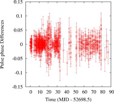
Figure 5: Plot of the pulse phase differences between contiguous intervals using our orbital parameters. The sinusoidal modulation is no more visible and there is no sign of the erratic behavior and long-term variations. This implies that our technique perfectly smooths out the erratic behavior and long-term variations.

where we fixed $d\varepsilon=d\omega=0$. We iterate this process until no residual are observed. In this way we find a good fit, corresponding to a $\chi^{2}/\textit{d.o.f.}$ of $864.2/790$; the best fit parameters are reported in Tab. 1. In Fig. 5) we show the phase differences obtained correcting the time series with our best-fit orbital solution. No orbital modulation is visible in this plot, and the amplitude of the oscillation is now much reduced with respect to that visible in Fig. 3 corresponding to the orbital solution given by Kirsch_04.

To verify that our orbital solution is indeed better than the orbital solution given by Kirsch_04 even during the times of the XMM observation we performed the following check. We looked in the RXTE observations for a time interval close in time to the time of the XMM observation; unfortunately there is not a complete superposition between the RXTE and the XMM observation (that starts at 52720.57 MJD and stops at 52720.68, for an exposure time of about 9.3 ks). We therefore took two RXTE observations ($80145-01-04-08$ and $80145-01-05-01$, the closest continuous observations to the XMM observation, which cover the time interval from 52718.94 MJD to 52719.11 MJD), corrected them alternatively with the Kirsch solution and our solution, respectively, and then performed a folding search around the expected value of the spin period. While the Kirsch solution gives a peak in the $\chi^{2}$ curve of about $150-200$, our solution gives a peak in the $\chi^{2}$ curve of about 1000, demonstrating that the periodic signal revealed on the time series corrected with our orbital solution is much stronger even in a time interval as close as possible to the XMM observation.

The method described above that we used to determine a precise orbital solution for XTE J1807–294 does not allow any study of the spin frequency and its derivative, since the long-term phase variations, which indeed give information on possible variations of the spin frequency during the outburst, are eliminated when we calculate the phase differences. Therefore, in order to perform a timing study of the spin frequency, we have to correct the entire time series of the RXTE observations with our best-fit orbital solution, and ri-calculate the phase delays, which are shown in Fig. 6. As it can be seen from the figure, the strong sinusoidal modulation visible in Fig. 1 is no more present. Moreover, our more precise orbital solution allows us to clearly detect the coherent pulsations up to 104 days since the start of the observation (June 12) with a detection confidence level of $3.6\;\sigma$, while between May 26 and June 10, although the source is still detectable, the pulsations are no more significantly detected. Long-term variations (a parabolic trend on which erratic fluctuations are superimposed) of the phases are again visible in this figure and are probably determined by the presence of a spin frequency derivative and/or an error in the spin frequency used to obtain the folded pulse profile, as well as by fluctuations of the phases on shorter timescales possibly related to phase shifts in the neutron star surface caused by variations of the X-ray flux. The discussion of these effects is beyond the scope of this paper and will be presented elsewhere (Riggio_07).

5 Conclusions

We have described a simple technique that permits to drastically reduce the presence of erratic behavior and long-term intrinsic variations of the pulse phase delays of the source, thus allowing to fit the residual orbital modulation of these phase delays, caused by errors in the previously reported orbital parameters, on a very long time-span and to obtain a much more precise measure of the orbital parameters. We applied this technique to the source XTE J1807–294, which shows the longest X-ray outburst observed by RXTE from an accreting millisecond pulsar. In this way we can fit the residual modulation of the phase differences over the whole time-span in which the coherent pulsations were significantly detected (about 100 days from the start of the outburst), obtaining a set of orbital parameters with a precision that is at least one order of magnitude better than the previously published orbital solutions for this source.

Once a good orbital parameters set is known, a detailed discussion of the spin period and its derivative is possible. However, this source also shows erratic fluctuations of the phases that are anticorrelated to variations in the X-ray flux, in a way that is similar to what is found by Papitto_07 for the source XTE J1814–338. A detailed discussion of these effects and a determination of the spin frequency and its derivative in XTE J1807–294 will be presented elsewhere (Riggio_07).

We acknowledge the use of RXTE data from the HEASARC public archive. This work was supported by the Ministero della Università e della Ricerca (MiUR) national program PRIN2005 2005024090$\_$004.

Table 1: Orbital Parameters for XTE J1807-294.

Parameter	Other Works	This Work
Orbital period, $P_{orb}$ (s)	2404.45(3)a	2404.41665(40)
Projected semi-major axis, $a_{x}\sin i$ (lt-ms)	4.8(1)b	4.819(4)
Ascending node passage, T⋆ a (MJD)	52720.67415(16)b	52720.675603(6)
Eccentricity, e	-	$<$ 0.0036
Spin frequency, $\nu_{0}$ (Hz)	190.623508(15)b	190.62350694(8)c

Errors are intended to be at $1\sigma$ c.l., upper limits are given at 95% c.l.

^aMarkwardt_iauc_03b.

^bKirsch_04.

^cRiggio_07.

Figure 1: Plot of the pulse phase delays obtained by epoch folding the events barycentered with respect the orbital parameters reported by Kirsch_04 on time intervals of $P_{orb}/6$. It is clearly visible a residual orbital modulation superimposed to the long-term, sometimes erratic, behavior of the phases.

Figure 2: Plot of the gain of the filter, that is the ratio between the amplitude of a sinusoidal input signal of period $P$ and the amplitude of the output sinusoidal signal when the time distance between two adjacent points is $\Delta t$.

Figure 3: The same as Figure 1 but plotting the pulse phase delays differences (instead of the pulse phase delays, see text). As can be seen the erratic behavior and long-term variations result strongly reduced. The linear decrease of the amplitude is a clear sign of an error on the $P_{orb}$.

Figure 4: Top: Detail of the pulse phase delays differences of Fig.3 between the days 10 and 11 from the start of the observation. As can be seen there is only a sinusoidal modulation and there is no sign of the erratic behavior. The dotted line is the best-fit model described in Eq.5. Bottom: Post-fit residuals with respect to the best-fit sinusoidal model.

Figure 6: Pulse Phase delays as a function of time of XTE J1807–294 obtained correcting the time series with our best fit orbital solution. The light curves are folded on a time interval of length $P_{orb}$. It is now apparent again the erratic behavior of the phases on characteristic timescales of at least several dozen of $P_{orb}$.