Transmission in double quantum dots in the Kondo regime: Quantum-critical transitions and interference effects

Abstract

We study the transmission through a double quantum-dot system in the Kondo regime. An exact expression for the transmission coefficient in terms of fully interacting many-body Green’s functions is obtained. By mapping the system into an effective Anderson impurity model, one can determine the transmission using numerical renormalization-group methods. The transmission exhibits signatures of the different Kondo regimes of the effective model, including an unusual Kondo phase with split peaks in the spectral function, as well as a pseudogapped regime exhibiting a quantum critical transition between Kondo and unscreened phases.

, and

1 Introduction

Semiconductor quantum dots have played a major role in the investigation of strongly correlated effects in nanoscale systems, as highlighted in the pioneering experiments on Kondo effect in these devices [1]. More recently, double-dot setups have been used to investigate two-impurity and two-channel Kondo physics [2]. These experimental developments have spurred great theoretical interest in double dots in the Kondo regime. In particular, studies of side-coupled [3] and parallel [4] dot configurations have been carried out.

Motivated by these accomplishments, we study transport properties of double quantum dots (DQDs) with one interacting dot (“dot 1”) coupled to a large dot, effectively noninteracting (“dot 2”, with energy $\varepsilon_{2}$). This seemingly simple setup can be described by an Anderson model coupled to a fermionic bath with a nonconstant density of states (DoS). Compared with the standard case of a metallic host (constant DoS), a nonconstant DoS leads to nontrivial new and interesting features in the many-body Kondo state.

As shown previously [5], a splitting the Kondo resonance appears when the DoS shows a sharp peak at the Fermi energy, while the Kondo singlet itself is preserved. The proposed DQD setup also allows for the appearance of a pseudogap in the effective DoS, leading to a critical transition between Kondo and non-Kondo phases. These phenomena substantially modify the spectral function of the interacting dot. We show here that another quantity, the transmission coefficient, can also be used to explore the critical transition and other features of this system.

We obtain an exact expression for the transmission coefficient $T(\omega$) in terms of the fully interacting many-body Green’s functions for the DQD system, which are then calculated within the numerical renormalization-group (NRG) framework. This approach allows us to fully describe the characteristics of the transmission coefficient in the different regimes mentioned above.

2 Model

The model describes the DQD setup depicted in Fig. 1: quantum dots $1$ (singly occupied with charging energy $U$ and energy $\varepsilon_{1}$) and $2$ (energy $\varepsilon_{2}$) are coupled to metallic leads ($\ell=L,R$) and to each other.

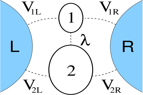
Figure 1: Schematic representation of the double-dot system.

The Hamiltonian is given by $H=H_{1}+H_{2}+H_{\mbox{\tiny Leads}}+H_{\mbox{\tiny Dot-Dot}}+H_{\mbox{\tiny Dot-Leads}}$, where

$$H_{\mbox{\tiny Leads}} = \sum_{{\bf k},\,\ell=L,R}\varepsilon_{\ell k}c^{\dagger}_{\ell{\bf k}\sigma}c^{\phantom{\dagger}}_{\ell{\bf k}\sigma}\,,$$

$$H_{i=1,2} = \varepsilon_{i}c^{\dagger}_{i\sigma}c^{\phantom{\dagger}}_{i\sigma}+\delta_{i,1}Un_{1\uparrow}n_{1\downarrow}\,,$$

$$H_{\mbox{\tiny Dot-Leads}} = \sum_{{\bf k},\,\ell=L,R}\left(V_{i\ell{\bf k}}c^{\dagger}_{i\sigma}c^{\phantom{\dagger}}_{\ell{\bf k}\sigma}+V^{*}_{i\ell{\bf k}\sigma}c^{\dagger}_{\ell{\bf k}\sigma}c^{\phantom{\dagger}}_{i\sigma}\right),$$

$$H_{\mbox{\tiny Dot-Dot}} = \lambda c^{\dagger}_{1\sigma}c^{\phantom{\dagger}}_{2\sigma}+\lambda^{*}c^{\dagger}_{2\sigma}c^{\phantom{\dagger}}_{1\sigma}\,.$$ (1)

The transmission amplitude for an electron tunneling from the left lead to the right lead can be obtained from the retarded Green’s function connecting the leads, $G_{L{\bf k}R{\bf k}^{\prime}}(\omega)\equiv\langle\langle c^{\phantom{\dagger}}_{L{\bf k}},\,c^{\dagger}_{R{\bf k}^{\prime}}\rangle\rangle$:

$$G_{L{\bf k}R{\bf k}^{\prime}}(\omega)=\sum_{i,j=1,2}g_{L{\bf k}}\;V^{*}_{iL{\bf k}}G_{ij}(\omega)V_{jR{\bf k}^{\prime}}\;g_{R{\bf k}^{\prime}}\,.$$ (2)

with $g_{\ell{\bf k}}\equiv(\omega^{+}-\varepsilon_{\ell k})^{-1}$. In the derivation of the expression above, we have used identities from the equations of motion for fermionic operators $c^{\phantom{\dagger}}_{a},\,c^{\dagger}_{b}$ in the frequency domain that include [6]:

$$\omega\,\langle\langle c^{\phantom{\dagger}}_{a}:c^{\dagger}_{b}\rangle\rangle_{\omega} = \langle[c^{\phantom{\dagger}}_{a},c^{\dagger}_{b}]_{\eta}\rangle+\langle\langle[c^{\phantom{\dagger}}_{a},H]_{-}:c^{\dagger}_{b}\rangle\rangle\;,$$

$$\omega\,\langle\langle c^{\phantom{\dagger}}_{a}:c^{\dagger}_{b}\rangle\rangle_{\omega} = \langle[c^{\phantom{\dagger}}_{a},c^{\dagger}_{b}]_{\eta}\rangle-\langle\langle c^{\phantom{\dagger}}_{a}:[c^{\dagger}_{b},H]_{-}\rangle\rangle\,.$$ (3)

In the wide-band limit $D\gg|\omega|$, where $D$ is the half-bandwidth, we approximate $V_{i\ell{\bf k}}\equiv V_{i\ell}$ (${\bf k}$-independent couplings) and $\sum_{{\bf k}}(\omega^{+}-\varepsilon_{k})^{-1}\rightarrow-i\pi\rho_{0}$ (where the same DoS $\rho_{0}$ is assumed for each lead) and one obtains the following expression for the energy-dependent transmission from $L$ to $R$:

$$T(\omega) = \sum_{{\bf k},{\bf k}^{\prime}}G_{L{\bf k}R{\bf k}^{\prime}}(\omega)=2\pi\rho_{0}\!\!\!\!\sum_{i,j=1,2}\!\!V^{*}_{iL}G_{ij}(\omega)V_{jR}\,.$$ (4)

In the following, we assume a symmetric configuration $V_{iR}=V_{iL}=V_{i}/\sqrt{2}$ with real values for the couplings for simplicity. Defining $\Delta_{i}\equiv\pi\rho_{0}V^{2}_{i}$ and $\Delta_{12}\equiv\pi\rho_{0}V_{1}V_{2}$, $T(\omega)$ can be written in a compact form:

$$T(\omega) = \Delta_{1}G_{11}+\Delta_{2}G_{22}+\Delta_{12}\left(G_{12}+G_{21}\right).$$ (5)

All $G_{ij}$ in (5) are fully interacting Green’s functions. Interaction effects are introduced into the dot-2 Green’s function by direct and indirect (via the leads) tunneling to dot 1. The identities (3) can be used to establish the relations

$$G_{22}(\omega) = G^{(0)}_{22}(\omega)+G_{21}(\omega)G_{11}(\omega)G_{12}(\omega)\,,$$

$$G_{12}(\omega) = G^{(0)}_{22}(\omega)\left(\lambda-i\Delta_{12}\right)G_{11}(\omega)\,.$$ (6)

Notice that for real couplings, $G_{12}(\omega)=G_{21}(\omega)$. These relationships in turn lead to an exact expression for the transmission involving only the noninteracting dot-2 Green’s function $G^{(0)}_{22}(\omega)=\left(\omega-\varepsilon_{2}+i\Delta_{2}\right)^{-1}$ and the fully interacting dot-1 Green’s function $G_{11}(\omega)\equiv\langle\langle c^{\phantom{\dagger}}_{1\sigma}\!:\!c^{\dagger}_{1\sigma}\rangle\rangle$:

$$T(\omega) = \Delta_{1}G_{11}(\omega)+2\Delta_{12}\left[G^{0}_{22}(\omega)(\lambda-i\Delta_{12})G_{11}(\omega)\right]$$

$$+ \Delta_{2} G^{0}_{22}(\omega)\left[1+G^{0}_{22}(\omega)(\lambda-i\Delta_{12})^{2}G_{11}(\omega)\right].$$ (7)

The dot-1 Green’s function $G_{11}$ is obtained from NRG calculations in the following manner: Hamiltonian (1) is mapped [5] onto an Anderson impurity connected to an effective nonconstant DoS through a hybridization function

$$\Delta(\omega)=\pi\rho_{2}(\omega)\left[\lambda+(\omega-\varepsilon_{2})\sqrt{\Delta_{1}/\Delta_{2}}\,\right]^{2},$$ (8)

with $\rho_{2}(\omega)=\Delta_{2}/\{\pi[(\omega-\varepsilon_{2})^{2}+\Delta_{2}^{2}]\}$. In general, $\Delta(0)\neq 0$ gives the effective broadening of the single-particle Hubbard peaks in dot 1 produced by the coupling to the effective nonconstant DoS. Notice that, for $\Delta_{2},\lambda\rightarrow 0$ (single-dot case), $\Delta(0)\rightarrow\Delta_{1}$.

We focus on two limiting configurations. In the “side-dot” limit ($\Delta_{1}=0;\Delta_{2},\lambda\neq 0$), dot 1 is connected to the leads only by second-order tunneling processes mediated by dot 2, and $\Delta(\omega)$ has a Lorentzian form, with a peak of width $\Delta_{2}$ centered at $\varepsilon_{2}$. In the “parallel-dot” limit ($\Delta_{1},\Delta_{2}\neq 0;\lambda=0$), dot 1 and dot 2 are connected only by indirect tunneling through the leads. Now $\Delta(\omega)$ has an “inverted Lorentzian” shape, vanishing as $|\omega-\varepsilon_{2}|^{2}$ at $\omega=\varepsilon_{2}$; if dot 2 is in resonance with the leads ($\varepsilon_{2}=0$, the case assumed throughout the remainder of the paper), this corresponds to a pseudogap in the effective DoS with exponent $2$.

The spectral function $A_{11}(\omega)=-\pi^{-1}\mbox{Im }G_{11}(\omega)$ is obtained from the NRG spectra using the method described in Ref. [7]. In short, at each NRG iteration $N$, one collects partial information for the spectral function by approximating $A_{11}(\omega)=A^{N}_{11}(\omega)$ for $\omega_{N}<\omega\lesssim 10\omega_{N}$ where $\omega_{N}\approx D\Lambda^{-N/2}$ ($\Lambda>1$) is the characteristic energy scale at iteration $N$. A continuous function can be obtained by replacing the $\delta$-functions at energies $E_{n}$ entering the Lehmann expression by logarithmically broadened lines $\delta^{b}(\omega-E_{n})\propto\exp\left[-(\ln{\omega}-\ln{E_{n}})^{2}/b^{2}\right]$.

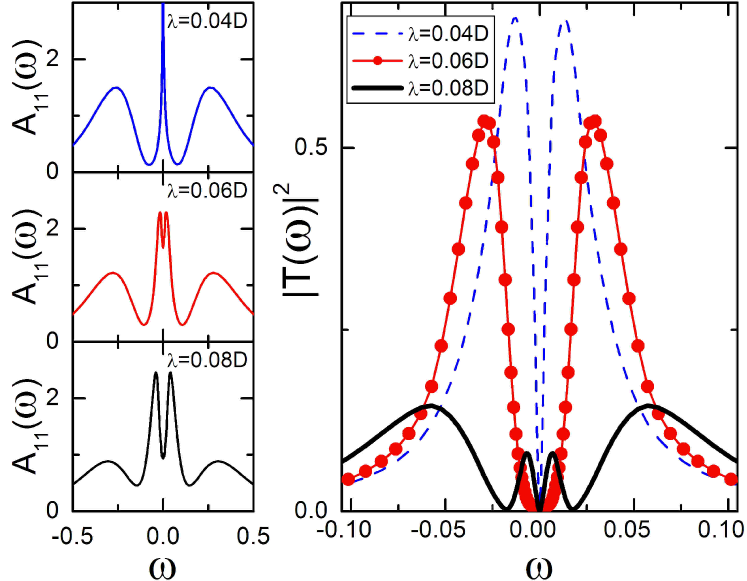
Figure 2: (color online) Spectral densities (left panels) and transmission amplitude (right panel) for the side dot configuration with $\varepsilon_{1}=-U/2$ and $\lambda=0.04D$ (dashed lines), $0.06D$ ($\bullet$) and $0.08D$ (thick solid line). Notice the appearance of secondary peaks in $|T(\omega)|^{2}$ as $\lambda$ increases.

Next, $\mbox{Re }G_{11}(\omega)$ is obtained from $A_{11}(\omega)$ via the appropriate Kramers-Kronig (KK) transformation. Because of the subtleties involved in the use of such transformations, we compared (i) the results of transforming $A_{11}(\omega)$ obtained numerically as described above with (ii) those from performing the KK at each NRG step, calculating $F_{N}(\omega)=\pi^{-1}\mathcal{P}\int d\omega^{\prime}A^{N}_{11}(\omega^{\prime})/\left(\omega^{\prime}-\omega\right)$ and then approximating $\mbox{Re }G_{11}(\omega)=-\pi^{-1}F_{N}(\omega)$ for $\omega_{N}<\omega\lesssim 10\omega_{N}$. We obtained qualitatively similar results with both methods, with better agreement for larger $b$ entering $\delta^{b}(\omega-E_{n})$ ($b=0.3$–$0.6$ for the results presented). For large $N$, an additional, broadening-independent estimate of $G_{11}(0)$ can be obtained from the expression [8] $F_{N}(0)=Z_{N}(0)^{-1}\sum_{n}\left(|\langle n|c_{1\sigma}|0\rangle|^{2}-|\langle 0|c_{1\sigma}|n\rangle|^{2}\right)/E^{N}_{n}$, where $E^{N}_{n}$, $|n\rangle_{N}$ and $Z_{N}(0)$ are, respectively, the eigenenergies, eigenstates and zero-temperature grand-canonical partition function at NRG iteration $N$, with $n=0$ representing the ground state.

3 Results

In the following, we take $U=0.5D$ and $\Delta_{2}=0.02D$. In the side-dot configuration considered, the effective dot-1 hybridization $\Delta(\omega)$ has a resonance of width $\Delta_{2}$ at the Fermi energy. Note that $\Delta(0)=\lambda^{2}/\Delta_{2}$, so that the Kondo temperature $T_{K}\propto e^{-1/\Delta(0)}$ will increase as $\lambda$ increases.

As previously shown [5], the presence of a resonance in the effective hybridization leads to a splitting in the spectral function for $\lambda\gtrsim\lambda^{*}$, where $\lambda^{*}$ is defined implicitly by $T_{K}(\lambda^{*},\Delta_{2})=\Delta_{2}$. This can be seen in the left panels of Fig. 2, for which $\lambda^{*}\sim 0.05D$.

The transmission amplitude is shown in the main panel of Fig. 2. At $\omega=0$, the Friedel sum rule requires that $\mbox{Im}G_{11}(0)=-\Delta_{2}/\lambda^{2}$. Substituting this result in Eq. (7) leads to $|T(0)|^{2}=0$ independently of $\lambda,\Delta_{2}$. The vanishing of transmission across the double-dot system is essentially an interference effect: the path going directly from the left lead to the right lead through dot 2 interferes destructively with the alternate path in which the electron tunnels in and out of dot 1.

Signatures of the splitting in the spectral density appear in the transmission amplitude at finite $\omega$. For increasing values of $\lambda$, the onset of the splitting in the spectral function (left panels in Fig. 2) is accompanied by the appearance of satellite peaks in $|T(\omega)|^{2}$ near $\omega=0$.

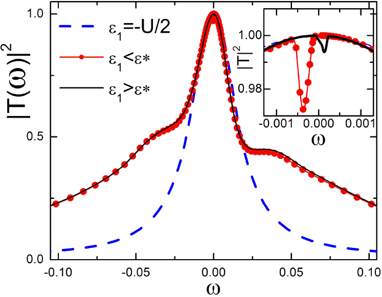
Figure 3: (color online) Transmission amplitude for the parallel configuration with $\Delta_{1}=0.05D$, and $\varepsilon_{1}=-U/2$ (dashed line) $-0.088U$ ($\bullet$) and $-0.086U$. The critical point is reached at $\varepsilon^{*}_{1}=-0.086524U$. Inset: A dip in $T(\omega)$ crosses $\omega=0$ due to the pseudogap-induced transition.

In the case of the dots in a parallel configuration, the situation is different, as shown in Fig. 3. Notice that $|T(0)|^{2}=1$ always, which is a direct consequence of the presence of the pseudogap in the hybridization function $\Delta(\omega)$. In the resulting effective pseudogapped Anderson model, the spectral density vanishes as $|\omega|^{2}$ at the Fermi energy. Thus, $\mbox{Im }G_{11}(0)=0$, effectively closing the transmission through dot 1 at the Fermi energy. In this regime, the transmission is dominated by the resonant tunneling through dot 2.

Important differences appear in particle-hole (p-h) symmetric and asymmetric regimes. In the p-h symmetric case ($\varepsilon_{1}=-U/2$, dashed lines in Fig. 3) the dot-1 spectral density varies as $\omega^{2}$ within a relatively large range $|\omega|<\Delta_{2}$ around the Fermi energy [5]. In this case, $|T(\omega)|^{2}$ is essentially a Lorentzian of width $\Delta_{2}$.

Away from p-h symmetry, a quantum critical point separating Kondo and non-Kondo phases can be reached [5]. Passage through the quantum critical point is reflected in position of a peak in the dot-1 spectral function at a frequency $\omega^{*}$ that crosses from $\omega^{*}>0$ in the Kondo phase to $\omega^{*}<0$ in the unscreened phase [9].

We find that the transition also has a signature in the transmission. The inset to Fig. 3 shows that the low-energy peak in $A_{11}$ translates into a dip in $|T(\omega)|^{2}$ at $\omega\approx\omega^{*}$—a dip that passes through the Fermi energy at the quantum critical point. The amplitude and width of this dip depend on structural parameters that should be tunable in experiments to enhance the feature. This opens interesting possibilities for controlled experimental study of a quantum phase transition through conductance measurements.

4 Conclusions

We have analyzed the electronic transmission in two different regimes of a double quantum-dot system. Utilizing an Anderson Hamiltonian and its exact solution using numerical renormalization group methods, one can determine the energy-dependent transmission function for the structure. As different geometries are explored, one can access an unusual Kondo regime with split peaks in the spectral function, as well as a Kondo system in a pseudogapped environment, allowing exploration of an interesting quantum critical transition. The transmission function exhibits clear signatures of these different Kondo regimes, opening the possibility of extensive experimental studies of their properties and response to different perturbations.

References

- [1] D. Goldhaber-Gordon etal., Nature 391, 156 (1998).
- [2] H. Jeong, A. M. Chang, and M. R. Melloch, Science 293, 2221 (2001); J. C. Chen, A. M. Chang, and M. R. Melloch, Phys. Rev. Lett. 92, 176801 (2004); N. J. Craig et al., Science 304, 565 (2004); A. Fuhrer et al., Phys. Rev. Lett. 93, 176803 (2004); R. Leturcq et al., Phys. Rev. Lett. 95, 126603 (2005); R. M. Potok et al., Nature 446, 169 (2007).
- [3] K. Kang, S. Y. Cho, J.-J. Kim, and S.-C. Shin, Phys. Rev. B 63, 113304 (2001); C. A. Busser, G. B. Martins, K. A. Al-Hassanieh, A. Moreo, E. Dagotto, Phys. Rev. B 70, 245303 (2004); P. S. Cornaglia and D. R. Grempel, Phys. Rev. B 71, 075305 (2005); P. Simon, J. Salomez, and D. Feinberg, Phys. Rev. B 73, 205325 (2006); R. Zitko and J. Bonca, Phys. Rev. B 73, 035332 (2006).
- [4] E. Vernek, N. Sandler, S. E. Ulloa, E. V. Anda, Physica E 34 608-611 (2006); R. Zitko and J. Bonca, Phys. Rev. B 74, 045312 (2006).
- [5] L. G. G. V. Dias da Silva, N. P. Sandler, K. Ingersent, and S. E. Ulloa, Phys. Rev. Lett. 97, 096603 (2006).
- [6] C. Lewenkopf, private communication.
- [7] R. Bulla, T. A. Costi, and D. Vollhardt, Phys. Rev. B 64, 045103 (2001).
- [8] J.-X Zhu, private communication.
- [9] M. Vojta and R. Bulla, Phys. Rev. B 65, 014511 (2001).