Horizons of Coalescing Black Holes on Eguchi-Hanson Space

Abstract

Using the numerical method, we study dynamics of coalescing black holes on the Eguchi-Hanson base space. Effects of a difference in spacetime topology on the black hole dynamics is discussed. We analyze appearance and disappearance process of marginal surfaces. In our calculation, the area of a coverall black hole horizon at the creation time in the coalescing black holes solutions on Eguchi-Hanson space is larger than that in the five-dimensional Kastor-Traschen solutions. This fact suggests that the black hole production on the Eguchi-Hanson space is easier than that on the flat space.

I Introduction

In the framework of the brane world scenario, higher dimensional black holes are expected to be produced in a future linear collider  Banks:1999gd ; Dimopoulos:2001en ; Giddings:2001bu ; IdaOdaPark1 ; IdaOdaPark2 ; IdaOdaPark3 . By observing physical phenomena associated with the black holes we might obtain evidences for existence of extra-dimensions. Such black holes, which evaporate by the Hawking radiation, are also expected to play crucial roles in the yet unaccomplished theoretical development to reconcile gravitational interactions with quantum description of nature.

So far, many authors have focused mainly on asymptotically flat and stationary higher dimensional black holes since they would be idealized models if such black holes are small enough for us to neglect the tension of a brane or the size of extra dimensions. It has been clarified that such asymptotically flat higher dimensional black hole solutions have richer structure than the four-dimensional one  Cai:2001su ; MyersPerry ; Emparan:2001wn ; Galloway:2005mf . However, there is no reason to restrict the asymptotic structures of higher dimensional spacetimes to the flat spacetime. Then, we do not have to restrict ourselves to black hole solutions with asymptotic flatness. In fact, higher dimensional black holes would admit a variety of asymptotic structures. For example, the black hole solutions in Kaluza-Klein theory admit the structure of a twisted ${\rm S}^{1}$ fiber bundle over four-dimensional Minkowski spacetime DM ; GW ; IM or a direct product of ${\rm S}^{1}$ and four-dimensional Minkowski spacetime MyersKKBH .

Recently, the coalescing black holes solutions on Eguchi-Hanson space (CBEH) are constructed in the five-dimensional Einstein-Maxwell theory with a positive cosmological constant Ishihara:2006ig . These solutions are asymptotic locally de Sitter spacetime; the topology of the radial coordinate $r=$const. surfaces is not a sphere $\rm S^{3}$ but the lens space. In this article, the behaviour of black holes at the early time and the late time are mainly discussed. The reason for this restriction is that it is easy to analyze the structure of solutions in such the region, which one can regard as that of the five-dimensional Reissner-Nordström-de Sitter solution (RNdS). As a result, it is clarified that the solutions describe the physical situation such that two black holes with the topology of $\rm S^{3}$ coalesce and change into a single black hole with the topology of the lens space $L(2;1)={\rm S}^{3}/{\mathbb{Z}}_{2}$.

Another solution of Einstein-Maxwell theory with a positive cosmological constant in arbitrary dimensions had been already found by London London:1995ib . These solutions, which are the generalization of the Kastor-Traschen solution Kastor:1992nn to higher dimensions, describe the dynamical situation such that the arbitrary number of multi-black holes with a spherical topology coalesce into a single black hole with a spherical topology in asymptotically de Sitter spacetime. Two black holes case of the five-dimensional Kastor-Traschen solutions (5DKT) describes that the two black holes with ${\rm S}^{3}$ coalesce into a single black hole with ${\rm S}^{3}$.

The purpose of this article is to investigate the global structure of the CBEH and the 5DKT by the numerical approach and to clarify the effects on coalescence of black holes brought about by the difference in asymptotic structure between both solutions. Following the numerical method in Refs. Nakao:1994mm ; Sasaki:1980 ; 1974AnPhy..83..449C , where they discussed how marginal surfaces evolve with time in the four-dimensional Kastor-Traschen solutions, we numerically investigate the existence and the time evolution of marginal surfaces. Especially, we focus on the appearance and disappearance process of marginal surfaces. We also discuss the time evolution of these areas.

The rest of this article is organized as follows. In Sec. II, we review the CBEH and the 5DKT. We show the method to search for marginal surfaces in Sec. III. Then, time sequence of marginal surfaces and these areas are shown in Sec. IV. Sec. V is devoted to the summary and discussion.

II Brief Review

II.1 five-dimensional Kastor-Traschen solutions

First, let us consider the 5DKT London:1995ib , namely, the black hole solutions on a flat base space. Especially, we concentrate on the solution with two black holes whose masses are $m_{1}$ and $m_{2}$ at early time

$$ds^{2}=a^{2}\left[-H_{\rm KT}^{-2}d\tau^{2}+H_{\rm KT}\left(dr^{2}+r^{2}d\Omega^{2}_{\rm S^{3}}\right)\right],$$ (1)

where $H_{\rm KT}$ is given by

$$H_{\rm KT}=\lambda\tau+\frac{m_{1}}{|\mbox{\boldmath{$r$}}-\mbox{\boldmath{$r$}}_{1}|^{2}}+\frac{m_{2}}{|\mbox{\boldmath{$r$}}-\mbox{\boldmath{$r$}}_{2}|^{2}},$$ (2)

with the position vector on the four-dimensional Euclid space $r$. $\bm{r}_{1}$ and $\bm{r}_{2}$ are the positions of point sources. We can set $\mbox{\boldmath{$r$}}_{1}=(0,0,0,1)$ and $\mbox{\boldmath{$r$}}_{2}=(0,0,0,-1)$ without a loss of generality.

II.1.1 Early time

Let us focus on the neighbourhood of $\mbox{\boldmath{$r$}}=\mbox{\boldmath{$r$}}_{i}~{}(i=1,2)$. In the new coordinate $\tilde{r}=|\mbox{\boldmath{$r$}}-\mbox{\boldmath{$r$}}_{i}|$, we can write the metric (1) as

$$ds^{2} \simeq a^{2}\left[-\biggl{(}\lambda\tau+\frac{m_{i}}{\tilde{r}^{2}}\biggr{)}^{-2}d\tau^{2}+\biggl{(}\lambda\tau+\frac{m_{i}}{\tilde{r}^{2}}\biggr{)}\biggl{\{}d\tilde{r}^{2}+\tilde{r}^{2}d\Omega_{\rm S^{3}}^{2}\biggr{\}}\right],$$ (3)

where $d\Omega_{\rm S^{3}}^{2}$ is the metric of a unit three-sphere. This is identical to the metric of the RNdS with mass parameter $m_{i}$ except for the conformal factor $a^{2}$ which does not contribute to the horizon condition $\theta_{\rm out}=0$, where $\theta_{\rm out}$ is the out-going null expansion on the $\tau=$const and $\tilde{r}=$const surface.

For this metric, let us introduce a variable $x:=\lambda\tau\tilde{r}^{2}$, and then horizons occur at $x$ satisfying

$$\lambda^{2}(x+m_{i})^{3}-4x^{2}=0.$$ (4)

For $m_{i}<16/(27\lambda^{2})$, there are three horizons, i.e., the inner and outer black hole horizons and the de Sitter horizon, which correspond to the three real roots $x_{\rm in}[m_{i}]<x_{\rm BH}[m_{i}]<x_{\rm dS}[m_{i}]$, respectively.

If $m_{i}<16/(27\lambda^{2})~{}(i=1,2)$, the horizon radius $\tilde{r}_{\rm BH}^{2}:=x_{\rm BH}[m_{i}]/(\lambda\tau)$ satisfy $\tilde{r}_{\rm BH}\ll|\mbox{\boldmath{$r$}}_{i}|=1$ at an early time $\tau\ll 0$. This fact means that we can find an approximately spherical and sufficiently small black hole horizon around $\mbox{\boldmath{$r$}}=\mbox{\boldmath{$r$}}_{i}$. Hence, an outer trapped region always exists around ${\bm{r}}={\bm{r}}_{i}$

II.1.2 Late time

Next, we study the asymptotic behaviour of the metric for large $r:=|{\bm{r}}|$, where we assume that $r$ is much larger than the coordinate distance $|{\bm{r}_{1}}-{\bm{r}_{2}}|=2$ between the two masses $m_{1}$ and $m_{2}$. Then, the metric takes the following form,

$$ds^{2} \simeq a^{2}\left[-\biggl{(}\lambda\tau+\frac{m_{1}+m_{2}}{r^{2}}\biggr{)}^{-2}d\tau^{2}+\biggl{(}\lambda\tau+\frac{m_{1}+m_{2}}{r^{2}}\biggr{)}\biggl{\{}dr^{2}+r^{2}d\Omega_{\rm S^{3}}^{2}\biggr{\}}\right].$$ (5)

This metric resembles that of the RNdS with mass equal to $m_{1}+m_{2}$. If we assume $m_{1}+m_{2}<16/(27\lambda^{2})$, the horizon radius $r_{\rm BH}^{2}:=x_{\rm BH}[m_{1}+m_{2}]/(\lambda\tau)$ satisfy $r_{\rm BH}\gg|\mbox{\boldmath{$r$}}_{1}-\mbox{\boldmath{$r$}}_{2}|=2$ at late time $\tau\to-0$. Then the approximate form of the metric (5) is valid around $r=r_{\rm BH}$. Hence, an approximately spherical black hole horizon can be found around $r=r_{\rm BH}$. in the metric (1).

II.2 Black holes on Eguchi-Hanson base space

Second, we give the brief review on the CBEH Ishihara:2006ig whose metric is given by

$$ds^{2}=a^{2}\left[-H_{\rm EH}^{-2}d\tau^{2}+\frac{1}{8}H_{\rm EH}\left\{V^{-1}dR^{2}+V^{-1}R^{2}d\Omega_{\rm S^{2}}^{2}+V\left(d\psi+\omega_{\phi}d\phi\right)^{2}\right\}\right],$$ (6)

where

$$H_{\rm EH} = \lambda\tau+\frac{2m_{1}}{\left|\mbox{\boldmath{$R$}}-\mbox{\boldmath{$R$}}_{1}\right|}+\frac{2m_{2}}{\left|\mbox{\boldmath{$R$}}-\mbox{\boldmath{$R$}}_{2}\right|},$$ (7)

$$V^{-1} = \frac{1}{\left|\mbox{\boldmath{$R$}}-\mbox{\boldmath{$R$}}_{1}\right|}+\frac{1}{\left|\mbox{\boldmath{$R$}}-\mbox{\boldmath{$R$}}_{2}\right|},$$ (8)

$$\omega_{\phi} = \frac{z-1}{\left|\mbox{\boldmath{$R$}}-\mbox{\boldmath{$R$}}_{1}\right|}+\frac{z+1}{\left|\mbox{\boldmath{$R$}}-\mbox{\boldmath{$R$}}_{2}\right|},$$ (9)

$$d\Omega_{\rm S^{2}}^{2} = d\theta^{2}+\sin^{2}\theta d\phi^{2},$$ (10)

and $\mbox{\boldmath{$R$}}=(R\sin\theta\cos\phi,R\sin\theta\sin\phi,R\cos\theta)$ is the position vector on the three-dimensional Euclid space and positions of point sources $\mbox{\boldmath{$R$}}_{1}$ and $\mbox{\boldmath{$R$}}_{2}$ are set to be $(0,0,1)$ and $(0,0,-1)$. The range of angular coordinates is defined by $0\leq\theta\leq\pi$, $0\leq\phi\leq 2\pi$ and $0\leq\psi\leq 4\pi$. This metric is given by equation (9) in Ref.Ishihara:2006ig , rewriting as $R\rightarrow aR$, $\tau\rightarrow a\tau$, $\lambda\rightarrow\lambda/a$, $m_{1}\rightarrow a^{2}m_{1}$ and $m_{2}\rightarrow a^{2}m_{2}$. This is a solution of the five-dimensional Einstein equation with a positive cosmological constant and the Maxwell equation with a gauge potential one-form given by

$$\quad\bm{A}=\pm\frac{\sqrt{3}}{2}aH_{\rm EH}^{-1}d\tau.$$ (11)

In order to focus on the coalescence of two black holes, we consider only the contracting phase $\lambda<0$. Though $\tau$ runs the range $(-\infty,\infty)$, in this article we investigate only the region $-\infty<\tau\leq 0$.

II.2.1 Early time

First, let us focus on the neighbourhood of ${\bm{R}}={\bm{R}_{i}}\ (i=1,2)$. In terms of the new coordinate $\bar{r}^{2}:=|\mbox{\boldmath{$R$}}-\mbox{\boldmath{$R$}}_{i}|/2$, the metric can be written in the form,

$$ds^{2}\simeq a^{2}\left[-\left(\lambda\tau+\frac{m_{i}}{\bar{r}^{2}}\right)^{-2}d\tau^{2}+\left(\lambda\tau+\frac{m_{i}}{\bar{r}^{2}}\right)\left\{d\bar{r}^{2}+\frac{\bar{r}^{2}}{4}d\Omega_{{\rm S}^{2}}^{2}+\frac{\bar{r}^{2}}{4}\left(d\psi+\cos\theta d\phi\right)^{2}\right\}\right].$$ (12)

This is equivalent to the metric of the the RNdS which has the mass equal to $m_{i}$ written in the cosmological coordinate. Hence like the 5DKT, we can conclude that a nearly spherical and small black hole horizon can be found around $\mbox{\boldmath{$R$}}=\mbox{\boldmath{$R$}}_{i}$ in the metric (1) at the early time, and sufficiently small spheres with the topology of $S^{3}$ centered at ${\bm{R}}={\bm{R}}_{i}$ are always outer trapped.

II.2.2 Late time

Next, we study the asymptotic behaviour of the metric (6) in the region where $R$ is much larger than the coordinate distance $|{\bm{R}_{1}}-{\bm{R}_{2}}|=2$. Here, let us introduce a new coordinate $\hat{r}^{2}:=R$, and then the metric takes the following form

$$ds^{2}\simeq a^{2}\left[-\left(\lambda\tau+\frac{m}{\hat{r}^{2}}\right)^{-2}d\tau^{2}+\left(\lambda\tau+\frac{m}{\hat{r}^{2}}\right)\left\{d\hat{r}^{2}+\frac{\hat{r}^{2}}{4}d\Omega_{\rm S^{2}}^{2}+\frac{\hat{r}^{2}}{4}\left(\frac{1}{2}d\psi+\cos\theta d\phi\right)^{2}\right\}\right],$$ (13)

where $m=2(m_{1}+m_{2})$. This resembles the metric of the RNdS solution with mass equal to $m$, and if we assume $m<16/(27\lambda^{2})$, a nearly spherical black hole horizon can be found in the metric (6) with $\hat{r}=r_{\rm BH}[m]$ at late time $\tau\to-0$.

However, we note that the metric form of (13) differ from that of the RNdS solution in the following point; Each $\hat{r}={\rm const}$ surface is topologically the lens space $L(2;1)={\rm S}^{3}/{\mathbb{Z}}_{2}$, while it is diffeomorphic to ${\rm S}^{3}$ in the RNdS solution. We can regard ${\rm S}^{3}$ and the lens space $L(2;1)={\rm S}^{3}/{\mathbb{Z}}_{2}$ as examples of Hopf bundles, i.e., ${\rm S}^{1}$ bundle over ${\rm S}^{2}$. The difference between these metrics appears in Eqs.(12) and (13): $d\psi$ in the metric (12) is replaced by $d\psi/2$ in the metric (13). Therefore, at late time, the topology of the trapped surface is the lens space $L(2;1)={\rm S}^{3}/{\mathbb{Z}}_{2}$ in the metric (6).

II.3 Comparison

The above results suggest that both solutions describe the coalescence of black holes. (In fact, using the numerical techniques, Nakao et.al. showed that the four-dimensional Kastor-Traschen solutions describe such physical process Nakao:1994mm .) Between both solutions, there exists the essential difference, namely, in the 5DKT, two black holes with the topology of ${\rm S}^{3}$ coalesce into a single black hole with the topology of ${\rm S}^{3}$, while in the CBEH, two black holes with the topology of ${\rm S}^{3}$ coalesce and change into a single black hole with the topology of $L(2;1)={\rm S}^{3}/{\mathbb{Z}}_{2}$. In the next section, we investigate how two black holes coalesce in the two solutions by pursuing time evolution of marginal surfaces.

III Method to search for marginal surfaces

Here, we seek marginal surfaces on $\tau={\rm constant}$ surfaces, which are defined as surfaces of co-dimension two such that the out-going orthogonal null geodesics have zero convergence $\theta_{\rm out}$ on the surfaces. The metrics (1) and (16) are decomposed into the form

$$g_{ab}=-n_{a}n_{b}+h_{ab},$$ (14)

where $n^{a}:=H_{\rm EH,KT}a^{-1}(\partial/\partial\tau)^{a}$ and $h_{ab}$ denote the timelike unit vector normal to the $\tau={\rm constant}$ surfaces and the induced metric on the surfaces, respectively.

In our numerical computation, we use the coordinate system $(\tau,z,\rho,\phi,\psi)$. The metric (1) is written as

$$ds^{2}=a^{2}\left[-H_{\rm KT}^{-2}d\tau^{2}+H_{\rm KT}\left\{dz^{2}+d\rho^{2}+\rho^{2}\left(d\phi^{2}+\sin^{2}\phi d\psi^{2}\right)\right\}\right],$$ (15)

in this coordinate system, and the metric (6) is written as

$$ds^{2}=a^{2}\left[-H_{\rm EH}^{-2}d\tau^{2}+\frac{1}{8}H_{\rm EH}\left\{V^{-1}\left(dz^{2}+d\rho^{2}+\rho^{2}d\phi^{2}\right)+V\left(d\psi+\omega_{\phi}d\phi\right)^{2}\right\}\right].$$ (16)

Let $s^{a}$ be the spacelike unit vector normal to such marginal surfaces on the $\tau=$constant surfaces, and consider the marginal surfaces as $(z,\rho,\phi,\psi)=\left(z(v),\rho(v),\phi,\psi\right)$, i.e., they are parameterized by $v,\phi$ and $\psi$ on the $\tau=$constant surfaces. Then, the metric $h_{ab}$ can be written on the following form

$$h_{ab}=s_{a}s_{b}+\delta_{ij}(e^{i})_{a}(e^{j})_{b},$$ (17)

where $\delta_{ij}={\rm diag}(1,1,1)$ and $(e_{i})^{a}\ (i=1,2,3)$ are triplet bases on the marginal surface. In the case of the CBEH, we can set $s^{a}$ and $(e_{i})^{a}$ in the forms

$$(e_{1})^{a}=\frac{2\sqrt{2V}}{a\sqrt{H_{\rm EH}(\dot{\rho}^{2}+\dot{z}^{2})}}\left(\dot{z}\left(\frac{\partial}{\partial z}\right)^{a}+\dot{\rho}\left(\frac{\partial}{\partial\rho}\right)^{a}\right),$$ (18)

$$(e_{2})^{a}=\frac{2\sqrt{2V}}{a\sqrt{H_{\rm EH}(\rho^{2}+\omega_{\phi}^{2}V^{2})}}\left(\frac{\partial}{\partial\phi}\right)^{a},$$ (19)

$$(e_{3})^{a}=\frac{2\sqrt{2}}{a\rho\sqrt{H_{\rm EH}V}}\left(\frac{-\omega_{\phi}V^{2}}{\sqrt{\rho^{2}+\omega_{\phi}^{2}V^{2}}}\left(\frac{\partial}{\partial\phi}\right)^{a}+\sqrt{\rho^{2}+\omega_{\phi}^{2}V^{2}}\left(\frac{\partial}{\partial\psi}\right)^{a}\right),$$ (20)

$$s^{a}=\pm\frac{2\sqrt{2V}}{a\sqrt{H_{\rm EH}(\dot{\rho}^{2}+\dot{z}^{2})}}\left(\dot{\rho}\left(\frac{\partial}{\partial z}\right)^{a}-\dot{z}\left(\frac{\partial}{\partial\rho}\right)^{a}\right),$$ (21)

where the sign $\pm$ of $s^{a}$ should be chosen so that $s^{a}$ directs outward. On the other hand, in the case of the 5DKT, we can set these vectors in the forms

$$(e_{1})^{a}=\frac{1}{a\sqrt{H_{\rm KT}(\dot{\rho}^{2}+\dot{z}^{2})}}\left(\dot{z}\left(\frac{\partial}{\partial z}\right)^{a}+\dot{\rho}\left(\frac{\partial}{\partial\rho}\right)^{a}\right),$$ (22)

$$(e_{2})^{a}=\frac{1}{a\rho\sqrt{H_{\rm KT}}}\left(\frac{\partial}{\partial\phi}\right)^{a},$$ (23)

$$(e_{3})^{a}=\frac{1}{a\rho\sqrt{H_{\rm KT}}\sin\phi}\left(\frac{\partial}{\partial\psi}\right)^{a},$$ (24)

$$s^{a}=\pm\frac{1}{a\sqrt{H_{\rm KT}(\dot{\rho}^{2}+\dot{z}^{2})}}\left(\dot{\rho}\left(\frac{\partial}{\partial z}\right)^{a}-\dot{z}\left(\frac{\partial}{\partial\rho}\right)^{a}\right).$$ (25)

The expansion $\theta_{\rm out}$ of the null congruence which is normal to the marginal surface is given by

$$\theta_{\rm out}=(h^{ab}-s^{a}s^{b})\nabla_{b}(n_{a}+s_{a})=-\sum_{i=1,2,3}s_{a}(e_{i})^{b}D_{b}(e_{i})^{a}+s^{a}s^{b}k_{ab}-{\rm tr}k,$$ (26)

where $k$ is the trace of the extrinsic curvature $k_{ab}$ of the $\tau=$constant surface. By the definition of a marginal surface, the expansion vanishes $\theta_{\rm out}=0$ on the surface. On the other hand, the expansion of the ingoing null congruence which is normal to the marginal surface is given by

$$\theta_{\rm in}=(h^{ab}-s^{a}s^{b})\nabla_{b}(n_{a}-s_{a})=\sum_{i=1,2,3}s_{a}(e_{i})^{b}D_{b}(e_{i})^{a}+s^{a}s^{b}k_{ab}-{\rm tr}k.$$ (27)

Since $\theta_{\rm out}$ vanishes on the marginal surface by its definition, we have

$$\theta_{\rm in}=\theta_{\rm in}+\theta_{\rm out}=2s^{a}s^{b}k_{ab}-2{\rm tr}k=\frac{3\lambda}{a}<0.$$ (28)

Equations (18)-(21) or Eqs.(22)-(25) with Eq.(26) gives a second-order ordinary differential equation

$$\theta_{\rm out}\left(\ddot{z},\ddot{\rho},\dot{z},\dot{\rho}\right)=0$$ (29)

for marginal surfaces on $\rho-z$ plane. We find smooth closed curves on the $\rho-z$ plane, $\rho=\rho(v),~{}z=z(v)$, satisfying Eq.(29). It should be noted that Eq.(29) does not depend on the parameter $a$. By use of the freedom in the choice of the parameter $v$, following CadezNakao:1994mm ; 1974AnPhy..83..449C , we fix $v$ by

$$\dot{z}^{2}+\dot{\rho}^{2}=\left(\frac{8V}{H_{\rm EH}}\right)^{2},$$ (30)

in the case of the CBEH, and

$$\dot{z}^{2}+\dot{\rho}^{2}=H_{\rm KT}^{-2}.$$ (31)

in the case of the 5DKT.

Using these parametrization (30) and (31) of $v$ and imposing the equations on the boundary conditions $\dot{z}=0$ at $z$-axis, we can numerically search for marginal surfaces.

IV Time evolution of horizons

IV.1 Marginal Surfaces

We would like to pursue how two black holes evolve with time and coalesce for both solutions. We restrict the range of the mass parameters to

$$m_{1}+m_{2}<\frac{8}{27\lambda^{2}}$$ (32)

so that a black hole horizon exists after the coalescence. In this article, we consider the case where two black holes at early time have equal masses and we set them to be $m_{1}=m_{2}=1/(8\lambda^{2})$ and $\lambda=-1/(2\sqrt{2})$ for both solutions. Under this assumption, since there is a reflection symmetry $z\to-z$, it is sufficient to consider only the region of $z\geq 0$. In general, several marginal surfaces exist on each time slice. We label each marginal surface which corresponds to a black hole horizon and de Sitter horizon at the early time as ${\rm BH_{E}}$ and ${\rm dS}_{\rm E}$, respectively, and label each marginal surface which corresponds to the black hole horizon and de Sitter horizon at the late time as ${\rm BH}_{\rm L}$ and ${\rm dS}_{\rm L}$, respectively. Some of marginal surfaces appear or disappear in pairs with another marginal surface. We label the marginal surfaces other than black hole horizons and de Sitter horizons as ${\rm MS}_{i}\ (i=1,2,\cdots)$. To avoid confusion, we do not depict marginal surfaces which are not related to the appearance and disappearance of ${\rm BH_{E}}$, ${\rm dS_{E}}$, ${\rm BH_{L}}$ and ${\rm dS_{L}}$.

FIG.1, FIG.2 and FIG.3 show the time sequence of marginal surfaces in the 5DKT. Before $\tau=-250$, there are two black hole horizons ${\rm BH_{E}}$, two de Sitter horizons ${\rm dS_{E}}$ enclosing each $\rm BH_{E}$. In addition, there is a marginal surface ${\rm MS_{1}}$ surrounding the two black hole horizons. After the lapse of time, at a time within the period $-160<\tau<-140$, another de Sitter horizon ${\rm dS_{L}}$ appears in pairs with another marginal surface ${\rm MS_{2}}$. After a brief interval, each ${\rm dS_{E}}$ disappears in pairs with ${\rm MS_{1}}$, and ${\rm MS_{2}}$ pinches off at a time in $-100<\tau<-80$. Finally, at a time in $-10<\tau<-5$, a new black hole horizon ${\rm BH_{L}}$ appears in pairs with a new marginal surface ${\rm MS_{3}}$, and then it asymptotically approaches to the black hole horizon of the RNdS with the mass parameter $m_{1}+m_{2}$.

Figure 1: Time evolution of marginal surfaces in the 5DKT: This figure shows when $\rm BH_{E}$, $\rm dS_{E}$, $\rm BH_{L}$, $\rm dS_{L}$ and three marginal surfaces $\rm MS_{1}$, $\rm MS_{2}$, $\rm MS_{3}$ exist. The vertical axis denotes the values of $\tau$. A pair of marginal surfaces connected by a dashed line appears or disappears at one time.

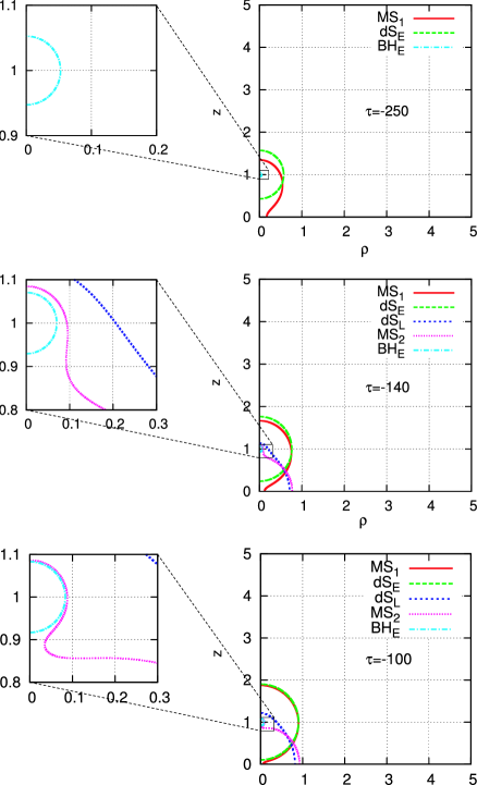
Figure 2: Time evolution of marginal surfaces in the 5DKT in $-250<\tau<-100$. The each left frame is the scaled-up figure of the region near ${\rm BH_{E}}$. At $\tau=-250$, ${\rm BH_{E}}$, ${\rm dS_{E}}$ and $\rm MS_{1}$ exist. ${\rm dS_{L}}$ and $\rm{MS_{2}}$ appear at same time during $-160<\tau<-140$.

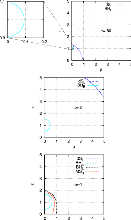
Figure 3: Time evolution of marginal surfaces in the 5DKT in $-80<\tau<-1$. The left frame at $\tau=-80$ is the scaled-up figure of the region near ${\rm BH_{E}}$. ${\rm dS_{E}}$ and $\rm{MS_{1}}$ disappear at same time and ${\rm MS_{2}}$ pinches off during $-100<\tau<-80$. Finally ${\rm MS_{3}}$ and $\rm{BH_{L}}$ appear at same time during $-2<\tau<-1$. In the figure at $\tau=-1$, ${\rm dS_{L}}$ exists in the outside the frame.

On the other hand, FIG.4, FIG.5 and FIG.6 show the time sequence of marginal surfaces in the CBEH. Before $\tau=-250$, there exist two ${\rm BH_{E}}$ and two ${\rm dS_{E}}$. At a time within the period $-230<\tau<-220$, ${\rm dS_{L}}$ appears in pairs with ${\rm MS_{1}}$. After a brief interval, ${\rm dS_{E}}$ disappears in pairs with ${\rm MS_{1}}$ at a time in $-140<\tau<-120$. Finally, ${\rm BH_{L}}$ appears in pairs with ${\rm MS_{2}}$ at a time in $-10<\tau<-5$, and ${\rm BH_{L}}$ approaches to a black hole horizon of the RNdS with the mass $2m_{1}+2m_{2}$ whose horizon topology is the lens space $L(2;1)={\rm S^{3}}/{\mathbb{Z}}_{2}$.

Figure 4: Time evolution of marginal surfaces in the CBEH: This figure shows when $\rm BH_{E}$, $\rm dS_{E}$, $\rm BH_{L}$, $\rm dS_{L}$ and two marginal surfaces $\rm MS_{1}$, $\rm MS_{2}$ exist. The vertical axis denotes the values of $\tau$. A pair of marginal surfaces connected by a dashed line appears or disappears at one time.

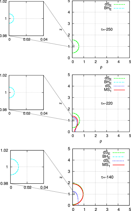
Figure 5: Time evolution of marginal surfaces in the CBEH in $-250<\tau<-140$. The each left frame is the scaled-up figure of the region near ${\rm BH_{E}}$. At $\tau=-250$, ${\rm BH_{E}}$ and ${\rm dS_{E}}$ exist. ${\rm MS_{1}}$ and $\rm{dS_{L}}$ appear at same time during $-250<\tau<-220$.

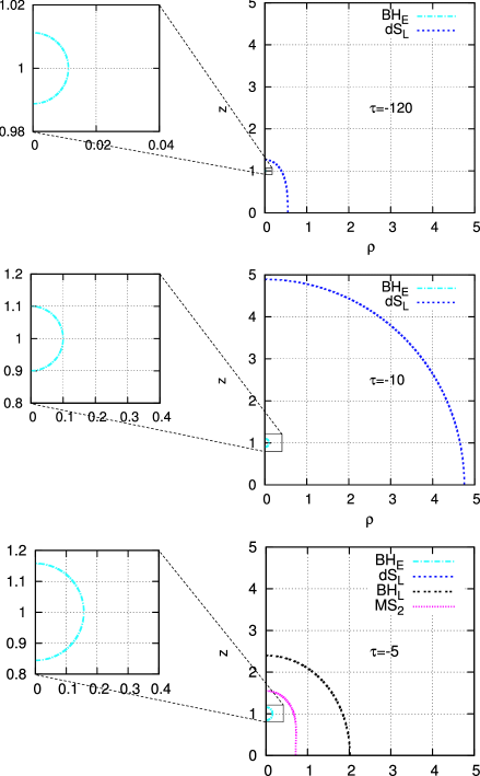
Figure 6: Time evolution of marginal surfaces in the CBEH in $-120<\tau<-5$. The each left frame is the scaled-up figure of the region near ${\rm BH_{E}}$. ${\rm dS_{E}}$ and $\rm{MS_{1}}$ disappear at same time during $-140<\tau<-120$. Finally ${\rm MS_{2}}$ and $\rm{BH_{L}}$ appear at same time during $-10<\tau<-5$. In the figure at $\tau=-5$, ${\rm dS_{L}}$ exists in the outside the frame.

We can see that two solutions differ in the number of marginal surfaces which are related to appearance and disappearance of $\rm dS_{E}$ and $\rm dS_{L}$. In each solution, the situation does not essentially depend on the choice of the parameters $m_{1}$, $m_{2}$ and $\lambda$. Hence, this result suggests that this difference dose not come from the difference in the choice of the parameters but in the asymptotic structures.

IV.2 Areas of horizons

First, for later convenience, we introduce the areas of horizons in the RNdS with the horizon topology of $L(n;1)=\rm S^{3}/{\mathbb{Z}}_{n}$ given by

$$\mathcal{A}_{n}(r_{\rm BH}[m^{\prime}])=\frac{2\pi^{2}a^{3}r^{3}_{\rm BH}[m^{\prime}]}{n}\left(\lambda\tau+\frac{m^{\prime}}{r^{2}_{\rm BH}[m^{\prime}]}\right)^{3/2},$$ (33)

$$\mathcal{A}_{n}(r_{\rm dS}[m^{\prime}])=\frac{2\pi^{2}a^{3}r^{3}_{\rm dS}[m^{\prime}]}{n}\left(\lambda\tau+\frac{m^{\prime}}{r^{2}_{\rm dS}[m^{\prime}]}\right)^{3/2},$$ (34)

where $m^{\prime}$ is the mass parameter in the metric form written by

$$ds^{2}=a^{2}\left[-\left(\lambda\tau+\frac{m^{\prime}}{r^{2}}\right)^{-2}d\tau^{2}+\left(\lambda\tau+\frac{m^{\prime}}{r^{2}}\right)\left\{dr^{2}+\frac{r^{2}}{4}d\Omega_{\rm S^{2}}^{2}+\frac{r^{2}}{4}\left(\frac{1}{n}d\psi+\cos\theta d\phi\right)^{2}\right\}\right].$$ (35)

In the previous work Ishihara:2006ig , we pointed out that after two black holes with the horizon topology of $\rm S^{3}$ coalesce, the area of the eventual single black hole in the CBEH is larger than that in the 5DKT, where we assume that each black hole in the CBEH has the same mass and area as that in the 5DKT. The difference is essentially due to the asymptotic structure. While the 5DKT is asymptotically de Sitter and each surface enclosing two black holes has the topological structure of ${\rm S}^{3}$, the topological structure of those in the CBEH is $L(2;1)={\rm S}^{3}/{\mathbb{Z}}_{2}$. In this sense, the CBEH is not asymptotically de Sitter but asymptotically locally de Sitter. Namely, the horizon radius of a black hole in the spacetime whose spatial infinity has the lens space $L(2;1)=\rm S^{3}/{\mathbb{Z}}_{2}$ becomes larger than that of the spacetime which has asymptotically Euclidean timeslices even if they have the same mass.

Using the results in the previous work, the ratios of areas of the black hole horizon and de Sitter horizon at the early time in the CBEH to those in the 5DKT become

$$\frac{\mathcal{A}^{\rm EH}_{\rm BH}}{\mathcal{A}^{\rm KT}_{\rm BH}}=\frac{\mathcal{A}_{1}(r_{\rm BH}[m_{1}])}{\mathcal{A}_{1}(r_{\rm BH}[m_{1}])}=1,\quad\frac{\mathcal{A}^{\rm EH}_{\rm dS}}{\mathcal{A}^{\rm KT}_{\rm dS}}=\frac{\mathcal{A}_{1}(r_{\rm dS}[m_{1}])}{\mathcal{A}_{1}(r_{\rm dS}[m_{1}])}=1,$$ (36)

where EH and KT denote the quantities associated with the CBEH and the 5DKT, respectively.

On the other hand, those at the late time become

$$\frac{\mathcal{A}^{\rm EH}_{\rm BH}}{\mathcal{A}^{\rm KT}_{\rm BH}}=\frac{\mathcal{A}_{2}(r_{\rm BH}[2(m_{1}+m_{2})])}{\mathcal{A}_{1}(r_{\rm BH}[m_{1}+m_{2}])}=C_{1},\quad\frac{\mathcal{A}^{\rm EH}_{\rm dS}}{\mathcal{A}^{\rm KT}_{\rm dS}}=\frac{\mathcal{A}_{2}(r_{\rm dS}[2(m_{1}+m_{2})])}{\mathcal{A}_{1}(r_{\rm dS}[m_{1}+m_{2}])}=C_{2},$$ (37)

where $C_{1}$ and $C_{2}$ are some constant determined by the values of $\lambda$, $m_{1}$ and $m_{2}$. In our setting, we find $C_{1}=0.332...$ and $C_{2}=2.350...$. Here, It should be noted that the area of the black hole horizon in the CBEH is larger than that in the 5DKT, but reversely the area of the de-Sitter horizon in the CBEH is smaller than that in the 5DKT.

Here, we numerically study how the areas of black hole horizons evolve with time in the 5DKT and the CBEH. The area of each marginal surface on $\tau$=constant surfaces is computed as

$${\cal A}^{\rm EH}=\frac{\pi^{2}a^{3}}{2\sqrt{2}}\int^{v_{1}}_{v_{2}}\rho\sqrt{\frac{H_{\rm EH}^{3}(\dot{z}^{2}+\dot{\rho}^{2})}{V}}dv,\quad{\cal A}^{\rm KT}=4\pi a^{3}\int^{v_{1}}_{v_{2}}\rho^{2}\sqrt{H_{\rm KT}^{3}(\dot{z}^{2}+\dot{\rho}^{2})}dv.$$ (38)

where $v_{1}$ and $v_{2}$ satisfy $z(v_{1})=z(v_{2})=0$.

FIG. 7 and FIG. 8 show the evolution of the areas of de Sitter horizons $\rm dS_{E}$ and $\rm dS_{L}$. FIG.9 and FIG. 10 show the time evolution of the areas of black hole horizons $\rm BH_{E}$ and $\rm BH_{L}$. The time evolution of the areas of $\rm BH_{E}$ and $\rm BH_{L}$ is shown in FIG.11. In fact, from these figures, we can confirm that these values of areas asymptotically approach to the values computed from Eqs. (36) and (37).

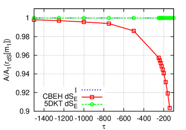
Figure 7: Time evolution of the area of ${\rm dS_{E}}$. The vertical axis denotes the area normalized by ${\cal A}_{1}(r_{\rm dS}[m_{1}])$.

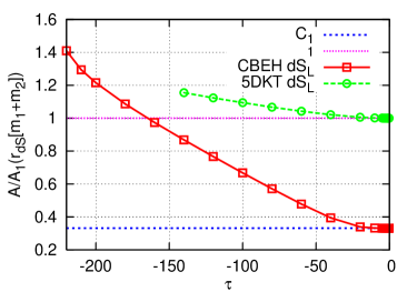
Figure 8: Time evolution of the area of ${\rm dS_{L}}$. The vertical axis denotes the area normalized by ${\cal A}_{1}(r_{\rm dS}[m_{1}+m_{2}])$.

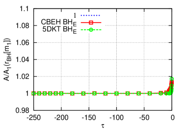
Figure 9: Time evolution of area of $\rm BH_{E}$s. The vertical axis denotes the area normalized by ${\cal A}_{1}(r_{\rm BH}[m_{1}])$.

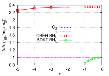
Figure 10: Time evolution of the areas of ${\rm BH_{L}}$s. The vertical axis denotes the area normalized by ${\cal A}_{1}(r_{\rm BH}[m_{1}+m_{2}])$.

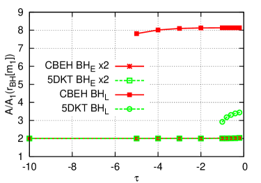
Figure 11: Time evolution of area of ${\rm BH_{E}}$ and ${\rm BH_{L}}$. The vertical axis denotes the area normalized by ${\cal A}_{1}(r_{\rm BH}[m_{1}])$.

From FIG.11, we see that the area of ${\rm BH_{L}}$ in the CBEH at the appearance is larger than that in the 5DKT. It suggests that the impact parameter at the appearance of black holes in a spacetime with asymptotically locally Euclidean timeslices may be larger than that in a spacetime with asymptotically Euclidean timeslices.

V Summary and Discussion

We have studied the evolution of marginal surfaces in the CBEH and the 5DKT. We have numerically searched for marginal surfaces in each time slice and calculated the areas of the horizons. Each marginal surface corresponding to the black hole or de Sitter horizon at the early or the late time appears or disappears in pairs with another marginal surface. We have shown the time evolution of the marginal surfaces in Figs 1, 2, 3, 4 , 4, 5 and 6.

The area at the appearance of the black hole enclosing both preexistent black holes in the CBEH is larger than that in the 5DKT. This suggests that the black hole production on the Eguchi-Hanson base space will be easier than that on the flat base space. It comes from the difference in the asymptotic structure between these solutions. The results of this article give us the suggestion that the black hole dynamics may be notably affected by the topological structure of the extra-dimensions. In the context of TeV gravity scenarios, the topology of the bulk space might be nontrivial. Hence if our living higher dimensional world admits the asymptotic structure of the lens space topology, the black hole production rate in the linear collider might give us some information or the restriction to the model about the asymptotic structure of the extra-dimensions.

Although throughout this article, we focus on the time evolution of marginal surfaces on a certain timeslice, finally, we also comment on the event horizon. In fact, we have searched for the event horizon numerically by tracing null geodesics from the sufficiently future region to the past region prep . ${\rm BH_{E}}$ and ${\rm BH_{L}}$ are almost identical to the cross sections of the event horizon with the timeslice $\tau=$constant surfaces at the sufficiently early and late time, respectively because the spacetime asymptotically becomes stationary in the sufficiently future and past regions.

From a general viewpoint, Siino discussed the topology change of an event horizon in the four-dimensional spacetime siino1 ; siino2 which is asymptotically stationary far in the future and showed that the non-trivial topology changes are caused by the set of endpoints of the event horizon, so-called, a crease set of the event horizon, where the event horizon is indifferentiable. Therefore, we expect that the difference between the topological structures of the crease sets will play a essential role in causing the difference in topology change in both solutions. In higher dimensional spacetimes, the structure of such crease sets is more complex than that in four-dimensions since the topology of an event horizon far in the future are not determined uniquely since the event horizons in higher dimensional stationary spacetimes can admit various topologies Cai ; HelfgottGalloway in contrast to four-dimensional ones, which is restricted only to ${\rm S}^{2}$ Hawking . The detailed analysis about the event horizon will be discussed in near future.

References

• (1) T. Banks and W. Fischler, hep-th/9906038.
• (2) S. Dimopoulos and G. Landsberg, Phys.Rev.Lett. 87, 161602 (2001).
• (3) S. B. Giddings and S. D. Thomas, Phys.Rev.D 65, 056010 (2002).
• (4) D. Ida, K. y. Oda and S. C. Park, Phys.Rev.D 67, 064025 (2003);
[Erratum-ibid. Phys.Rev.D 69, 049901 (2004)].
• (5) D. Ida, K. y. Oda and S. C. Park, Phys.Rev.D 71, 124039 (2005).
• (6) D. Ida, K. y. Oda and S. C. Park, Phys.Rev.D 73, 124022 (2006).
• (7) M. I. Cai and G. J. Galloway, Class.Quant.Grav. 18, 2707 (2001).
• (8) R. C. Myers and M. J. Perry, Annals Phys. 172, 304 (1986).
• (9) R. Emparan and H. S. Reall, Phys. Rev. Lett.  88, 101101 (2002).
• (10) G. J. Galloway and R. Schoen, Commun.Math.Phys. 266, 571, (2006).
• (11) P. Dobiasch and D. Maison, Gen.Rel.Grav. 14, 231 (1982).
• (12) G. W. Gibbons and D. L. Wiltshire, Annals Phys. 167, 201 (1986).
• (13) H. Ishihara and K. Matsuno, Prog. Theor. Phys. 116, 417 (2006).
• (14) R. C. Myers, Phys.Rev.D 35, 455 (1987).
• (15) H. Ishihara, M. Kimura and S. Tomizawa, Class.Quant.Grav. 23, L89 (2006).
• (16) L. A. J. London, Nucl.Phys.B 434, 709 (1995).
• (17) D. Kastor and J. Traschen, Phys.Rev.D 47, 5370 (1993).
• (18) A. Čadež, Annals Phys. 83, 449, (1974).
• (19) M. Sasaki, K. Maeda, S. Miyama and T. Nakamura, Prog.Theor.Phys. 63, 1051 (1980).
• (20) K. Nakao, T. Shiromizu and S. A. Hayward, Phys.Rev.D 52, 796, (1995).
• (21) Masashi Kimura, Hideki Ishihara, Ken Matsuno, Shinya Tomizawa, and Chul-Moon Yoo, Proc. of 17th JGRG
• (22) M. Siino, Phys.Rev.D 58, 104016, (1998).
• (23) M. Siino, Prog.Theor.Phys. 99, 1, (1998).
• (24) M. I. Cai and G. J. Galloway, Class.Quant.Grav. 18, 2707 (2001).
• (25) C. Helfgott, Y. Oz and Y. Yanay, JHEP 0602, 025 (2006);
G. J. Galloway and R. Schoen, Commun.Math.Phys. 266, 571, (2006);
G. J. Galloway, e-Print Archive: gr-qc/0608118.
• (26) S. W. Hawking, Commun. Math. Phys. 25, 152 (1972).