The optimal P3M algorithm for computing electrostatic energies in periodic systems

Abstract

We optimize Hockney and Eastwood’s Particle-Particle Particle-Mesh (P3M) algorithm to achieve maximal accuracy in the electrostatic energies (instead of forces) in 3D periodic charged systems. To this end we construct an optimal influence function that minimizes the RMS errors in the energies. As a by-product we derive a new real-space cut-off correction term, give a transparent derivation of the systematic errors in terms of Madelung energies, and provide an accurate analytical estimate for the RMS error of the energies. This error estimate is a useful indicator of the accuracy of the computed energies, and allows an easy and precise determination of the optimal values of the various parameters in the algorithm (Ewald splitting parameter, mesh size and charge assignment order).

I Introduction

Long range interactions are ubiquitously present in our daily life. The calculation of these interactions is, however, not an easy task to perform. One needs indeed to resort to specialized algorithms to overcome the quadratic scaling with the number of particles, as soon as the simulated system includes more than a few hundred particles, see for example the review of Arnold and Holm arnold05a . In Molecular Dynamics simulations, one is mainly interested in the accuracy of the force computation, since they govern the dynamics of the system. In contrast, in Monte Carlo (MC) simulations, the concern is to compute accurate energies. If the potential is of long range (e.g. a Coulomb potential or dipolar interaction), and one has chosen to use periodic boundary conditions, the computation of both observables is quite time consuming if one uses the traditional Ewald sum. Since the seminal work of Hockney and Eastwood HE it has been common to resort to a faster way of calculating the reciprocal space sum in the Ewald method with the help of Fast-Fourier-Transforms (FFTs). These algorithms are called mesh-based Ewald sums, and various variants exist DH . They all scale as $N\log N$ with the number of charged particles $N$, and the algorithms are nowadays routinely used in simulations of bio-systems, charged soft matter, plasmas, and many more areas. The most accurate variant is still the original method of Hockney and Eastwood, which they called particle-particle-particle-mesh (P3M), and into which various other improvements like the analytical differentiation used in other variants of the mesh-based Ewald sum SPME can be built in. In addition, an accurate error estimate for P3M exists, so that one can tune the algorithm to a preset accuracy, thus maximizing the computational efficiency before doing any simulations DH2 .

While in the standard P3M algorithmHE , the lattice Green function, called the “influence function”, is optimized to give the best possible accuracy in the forces, the electrostatic energy is usually calculated with the same force-optimized influence function. However, there are certainly situations where one needs a high precision of the energies, for instance in Monte Carlo simulations, and the natural question arises whether one can optimize the influence function to enhance the accuracy of the P3M energies. The main goal of this paper is to derive the energy-optimized influence function, and to derive an analytical estimate for the error in the P3M energies. This error estimate is a valuable indicator of the accuracy of the calculations and allows a straightforward and precise determination of the optimal values of the various parameters in the algorithm (Ewald splitting parameter, mesh size, charge assignment order).

The present derivation of the optimal influence function, and the associated error estimate, is concise and entirely self-contained. The present paper can thus also serve as a pedagogical introduction to the main ideas and mathematics of the P3M algorithm.

The paper is organized as follows. In Sec. II, we briefly review the ideas of the standard Ewald method and provide the most important formulae. In Sec. III, we derive direct and reciprocal space correction terms which compensate, on average, the effects of cut-off errors in the standard Ewald method. We interpret the formulae in terms of the direct and reciprocal space components of the Madelung energies of the ions. In Sec. IV, the calculation of the reciprocal energy according to the P3M algorithm (i.e. with a fast Fourier transform and an optimized influence function) is presented. The mathematical analysis of the errors introduced by the discretization on a grid is performed in Sec. V. This analysis is used in Sec. VI to derive the energy-optimized influence function and the associated RMS error estimate. The derivation shows that the P3M energies must be shifted to compensate for systematic cut-off and aliasing errors in the Madelung energies of the ions. Finally, our analytical results are tested numerically in Sec. VII.

II The Ewald sum

We consider a system of $N$ particles with charges $q_{i}$ at positions $\boldsymbol{r}_{i}$ in an overall neutral and (for simplicity) cubic simulation box of length $L$ and volume $V=L^{3}$. If periodic boundary conditions are applied, the total electrostatic energy of the box is given by

$$E=\frac{1}{2}\sum_{\boldsymbol{n}\in\mathbb{Z}^{3}}\sideset{}{{}^{{}^{\prime}}}{\sum}_{i,j=1}^{N}q_{i}q_{j}v(\boldsymbol{r}_{ij}+\boldsymbol{n}L),$$ (1)

where $v(\boldsymbol{r})={1}/{|\boldsymbol{r}|}$ is the Coulomb potential, $\boldsymbol{r}_{ij}=\boldsymbol{r}_{i}-\boldsymbol{r}_{j}$, and $\boldsymbol{n}$ is a vector with integer components that indexes the periodic images. The prime indicates that the (divergent) summand for $i=j$ has to be omitted when $\boldsymbol{n}=0$.

Because of the slow decay of the Coulomb interaction, the sum in (1) is only conditionally convergent: its value is not well defined unless one specifies the precise way in which the cluster of simulation boxes is supposed to fill $\mathbb{R}^{3}$. Often, one chooses a spherical order of summation, which is equivalent to the limit of a large, spherically bounded, regular grid of replicas of the simulation box, embedded in vacuum. The simulation box can then be pictured as the central LEGO brick in a huge ball made up of such bricks. If this “lego ball” is surrounded by a homogeneous medium with dielectic constant $\epsilon^{\prime}$ ($\epsilon^{\prime}=1$ if it’s vacuum) and if the simulation box has a net dipole moment $\boldsymbol{M}=\sum_{i}q_{i}\boldsymbol{r}_{i}$, the particles in the ball will feel a depolarizing field created by charges that appear on the surface of the uniformily polarized ball. It can be shown that the work done against this depolarizing field when charging up the system is

$$E^{(d)}=\frac{2\pi\boldsymbol{M}^{2}}{(1+2\epsilon^{\prime})L^{3}}$$ (2)

in the case of a spherical order of summation deLeeuw ; Caillol (for other summation orders, see the articles of SmithSmith88 and Ballenegger and Hansen BalHan ). The energy $E^{(d)}$ is contained, even if not easily seen, in the total electrostatic energy (1) (at least when $\epsilon^{\prime}=1$ since such a vacuum boundary condition was assumed in writing (1)). Obviously, the energy $E^{(d)}$ vanishes if we employ metallic boundary conditions defined by $\epsilon^{\prime}=\infty$.

The fact that $E^{(d)}$ depends on the order of summation, and hence on the shape of macroscopic sample under consideration, is a consequence of the conditional convergence of the sum (1). Due to the energy cost $E^{(d)}$, the fluctuations of the total dipole moment of the simulation box (and hence of the considered macroscopic sample) depend on the dielectric constant $\epsilon^{\prime}$ and on the shape of the sample. The energy $E^{(d)}$ is crucial to ensure, for example, that the dielectric constant $\epsilon$ of the simulated system obtained from the Kirkwood formula Kirkwood , which relates $\epsilon$ to the fluctuations of the total dipole moment, is independent of the choices made for the sample shape and for the dielectric boundary condition AlaBal ; BalHan2 .

Ewald’s method to compute the energy (1) is based on a decomposition of the Coulomb potential, $v(\boldsymbol{r})=\psi(\boldsymbol{r})+\phi(\boldsymbol{r})$, such that $\psi(\boldsymbol{r})$ contains the short-distance behavior of the interaction, while $\phi(\boldsymbol{r})$ contains the long-distance part of the interaction and is regular at the origin. The traditional way to perform this splitting is to define

$$\phi(\boldsymbol{r})=\mathrm{erf}(\alpha r)/r,\qquad r=|\boldsymbol{r}|,$$ (3)

and

$$\psi(\boldsymbol{r})=v(\boldsymbol{r})-\phi(\boldsymbol{r})=\mathrm{erfc}(\alpha r)/r$$ (4)

With this choice, $\psi(r)$ corresponds to the interaction energy between a unit charge at a distance $r$ from another unit charge that is screened by a neutralizing Gaussian charge distribution whose width is controlled by the Ewald length $\alpha^{-1}$. Following this decomposition of the potential, the electrostatic energy can be written in the well-known Ewald form Ewald21 ; deLeeuw :

$$E=E^{(r)}+E^{(k)}+E^{(d)}$$ (5)

where the real-space energy $E^{(r)}$ contains the contributions from short-range interactions $\psi(\boldsymbol{r})$, i.e.

$$E^{(r)}=\frac{1}{2}\sum_{\boldsymbol{n}\in\mathbb{Z}^{3}}\sideset{}{{}^{{}^{\prime}}}{\sum}_{i,j=1}^{N}q_{i}q_{j}\psi(\boldsymbol{r}_{ij}+\boldsymbol{n}L),$$ (6)

and the reciprocal space energy $E^{(k)}$ contains contributions from long-range interactions $\phi(\boldsymbol{r})$ (apart from the contributions that are responsible for the conditional convergence which are included in the term $E^{(d)}$ in (5)). The fact that the surface term (or “dipole term”) $E^{(d)}$ is independent of the Ewald parameter $\alpha$ shows that this contribution is not specific to the Ewald method, but more generally reflects the problems inherent to the conditional convergence of the $\boldsymbol{n}$ sum in Eq. (1). Contrary to $E^{(r)}$ which can be computed easily in real space thanks to the rapid decay of the $\psi$ interaction, $E^{(k)}$ is best computed in Fourier space, where it can be expressed as Ewald21

$$E^{(k)}=E^{(ks)}-E^{(s)}$$ (7)

where

$$E^{(ks)} =\frac{1}{2L^{3}}\sum_{\begin{subarray}{c}\boldsymbol{k}\in\mathbb{K}\\ \boldsymbol{k}\neq 0\end{subarray}}|\widetilde{\rho}(\boldsymbol{k})|^{2}\widetilde{\phi}(\boldsymbol{k})$$ (8)

$$E^{(s)} =Q^{2}\frac{\alpha}{\sqrt{\pi}}$$ (9)

with

$$Q^{2}=\sum_{i=1}^{N}q_{i}^{2}.$$ (10)

In (8), $\widetilde{\phi}(\boldsymbol{k})$ is the Fourier transform of the reciprocal interaction (3),

$$\widetilde{\phi}(\boldsymbol{k})=\int e^{-i\boldsymbol{k}\cdot\boldsymbol{r}}\phi(\boldsymbol{r})\hbox{d}\boldsymbol{r}=\frac{4\pi}{k^{2}}\exp(-k^{2}/4\alpha^{2}),$$ (11)

and $\widetilde{\rho}(\boldsymbol{k})$ is the Fourier transformed charge density

$$\widetilde{\rho}(\boldsymbol{k})=\sum_{i=1}^{N}q_{i}\,e^{-i\boldsymbol{k}\cdot\boldsymbol{r}_{i}}.$$ (12)

The sum in (8) is over wave vectors in the discrete set $\mathbb{K}=\{2\pi\boldsymbol{n}/L:\,\boldsymbol{n}\in\mathbb{Z}^{3}\}$. The term $\boldsymbol{k}=0$ is excluded in the sum because of the overall charge neutrality. The self-energy term $E^{(s)}$ compensates for the self-energies (the reciprocal interaction of each particle with itself $\frac{1}{2}q_{i}^{2}\phi(\boldsymbol{r}=\boldsymbol{0})=q_{i}^{2}\alpha/\sqrt{\pi}$) that are included in $E^{(ks)}$.

The energy (1) converges only for systems that are globally neutral. For systems with a net charge, the sum can be made convergent by adding a homogeneously distributed background charge which restores neutrality. In that case, an additional contribution Hummer

$$E^{(n)}=-\frac{\pi}{2\alpha^{2}L^{3}}\Big{(}\sum_{i=1}^{N}q_{i}\Big{)}^{2}$$ (13)

must be added to (5) to account for the interaction energies of the charges with the neutralizing background.

The reciprocal energy $E^{(ks)}$, defined by the Ewald formula (7), is the starting point of mesh-based Ewald sums, which are methods to compute efficiently that energy in many-particle systems. Notice that (7) can also be written in an alternative form in terms of a pair potential and a Madelung self-energy, see Appendix A. The inverse length $\alpha$ tunes the relative weight of the real space $E^{(r)}$ and the reciprocal space $E^{(k)}$ contributions to the energy, but the final result is independent of $\alpha$. In practice, $E^{(r)}$ and $E^{(k)}$ can be computed using cut-offs, because the sum over $\boldsymbol{n}$ in (6) and the sum over $\boldsymbol{k}$ in (8) converge exponentially fast. Typically, one chooses $\alpha$ large enough to employ the minimum image conventionAllen in Eq. (6).

At given real and reciprocal space cut-offs $r_{\mathrm{cut}}$ and $k_{\rm cut}$, there exists actually an optimal $\alpha$ such that the accuracy of the approximated Ewald sum is as high as possible. This optimal value can be determined with the help of the estimates for the cut-off errors derived by Kolafa and Perram KolPer , by demanding that the real and reciprocal space contributions to the error are equal. Kolafa and Perram’s root-mean-square error estimates are

$$\Delta E^{(r)}\simeq Q^{2}\sqrt{\frac{r_{c}}{2L^{3}}}\frac{e^{-\alpha^{2}r^{2}_{\mathrm{cut}}}}{(\alpha r_{\mathrm{cut}})^{2}}$$ (14)

and

$$\Delta E^{(k)}\simeq Q^{2}\alpha\,\frac{e^{-(\pi k_{\mathrm{cut}}/\alpha L)^{2}}}{\pi^{2}k_{\mathrm{cut}}^{3/2}}.$$ (15)

These error estimates make explicit the exponential dependence of the error on the real and reciprocal space cut-offs.

Formula (15) is actually valid only when a correction term (given by Eq. (24) below) is added, to compensate the systematic error that affects the reciprocal energies when the sum over wave vectors in (8) is truncated. The origin of this correction term is explained in detail in Sec. III. A similar term must also be introduced in the P3M algorithm when one computes the electrostatic energy. Similarly, the direct-space energy (6) also contains a systematic error when the pair-wise interaction is truncated at the cut-off distance $r_{\mathrm{cut}}$. The derivation in the next section will also provide a correction term for this effect.

To summarize, the final Ewald formula for the total electrostatic energy reads

$$\begin{split}E&=E^{(r)}&\mathrm{[eq.\eqref{U^r}]}\\ &+E^{(ks)}&\mathrm{[eq.\eqref{E^k}]}\\ &-E^{(s)}&\mathrm{[eq.\eqref{E^s}]}\\ &+E^{(d)}&\mathrm{[eq.\eqref{E^d}]}\\ &+E^{(n)}&\mathrm{[eq.\eqref{E^n}]}\\ \end{split}$$ (16)

Furthermore, when the sums in $E^{(r)}$ and $E^{(k)}$ are evaluated numerically using cut-offs, an additional correction term $E_{\mathrm{cut}}$, defined in Eq. (29) below, must be added to the truncated energy, as shown in the next section.

III Correction term for truncated Ewald sums

If we consider electroneutral systems where the charged particles are located at random, we expect the electrostatic energy to vanish on average, because there is an equal probability to find a positive or negative charge at any relative distance $r$. However, when periodic boundary conditions (PBC) are applied, the average energy of random systems does not vanish, because each charge interacts with its own periodic images (and with the uniform neutralizing background provided by the other charges).

Since this interaction energy $E_{\mathrm{img}}$ of an ion with its periodic images and with the neutralizing background does not depend on the position of the ion in the simulation box, it plays the role of a “self-energy”. We will refer to $E_{\mathrm{img}}$ as the Madelung (self-)energy of an ion, to avoid confusion with the self-energy $\frac{1}{2}q^{2}\phi(0)$ already defined in the Ewald method as the reciprocal interaction of a particle with itself.

We denote by angular brackets the average over the positions of the $N$ charged particles:

$$\left\langle{\cdots}\right\rangle=\frac{1}{V^{N}}\int_{V^{N}}\cdots\;\hbox{d}\boldsymbol{r}_{1}...\,\hbox{d}\boldsymbol{r}_{N}.$$ (17)

III.1 Madelung energy

The Madelung energy of an ion takes the form $E_{\mathrm{img}}=\frac{1}{2}q^{2}\zeta$, where $\zeta$ is a purely numerical factor in units of $1/L$ that depends only on the size and shape of the simulation box.

Let us calculate the average electrostatic energy of random charged systems in PBC, to find the value of $\zeta$ and derive a correction term for cut-off errors in truncated Ewald sums (some results derived here will be used in Sec. VI.1). On the one hand, the average Coulomb energy of the random systems is by definition $Q^{2}\zeta/2$, while on the other hand, it can be calculated as the sum of a direct space contribution $\left\langle{E^{(r)}}\right\rangle$ and a reciprocal space contribution $\left\langle{E^{(k)}}\right\rangle$. The average reciprocal energy is, using (9) and (8),

$$\left\langle{E^{(k)}}\right\rangle=\frac{1}{2L^{3}}\sum_{i,j}q_{i}q_{j}\sum_{\begin{subarray}{c}\boldsymbol{k}\in\mathbb{K}\\ \boldsymbol{k}\neq 0\end{subarray}}\left\langle{e^{-i\boldsymbol{k}\cdot(\boldsymbol{r}_{i}-\boldsymbol{r}_{j})}}\right\rangle\widetilde{\phi}(\boldsymbol{k})-Q^{2}\frac{\alpha}{\sqrt{\pi}}.$$ (18)

Since $\left\langle{\exp(-i\boldsymbol{k}\cdot\boldsymbol{r}_{j})}\right\rangle=\delta_{\boldsymbol{k},\boldsymbol{0}}$, all terms with $j\neq i$ vanish (this is due to the fact that the Ewald pair potential averages to zero, see Appendix A). By contrast, “self” terms ($i=j)$ remain and lead to

$$\left\langle{E^{(k)}}\right\rangle=\frac{Q^{2}}{2}\Big{(}\frac{1}{L^{3}}\sum_{\begin{subarray}{c}\boldsymbol{k}\in\mathbb{K}\\ \boldsymbol{k}\neq 0\end{subarray}}\widetilde{\phi}(\boldsymbol{k})-\frac{2\alpha}{\sqrt{\pi}}\Big{)}=\frac{Q^{2}}{2}\zeta^{(k)},$$ (19)

where the second equality defines $\zeta^{(k)}$. The average real-space energy of a single ion of charge $q_{i}$ in periodic random systems is

$$\left\langle{E_{i}^{(r)}}\right\rangle=\frac{q_{i}^{2}}{2}\Big{(}\sum_{\begin{subarray}{c}\boldsymbol{n}\in\mathbb{Z}^{3}\\ \boldsymbol{n}\neq 0\end{subarray}}\psi(\boldsymbol{n}L)-\frac{1}{L^{3}}\int_{\mathbb{R}^{3}}\psi(\boldsymbol{r})\,\hbox{d}^{3}\boldsymbol{r}\Big{)}$$ (20)

where the first term is the sum of the direct interactions of the ion with all its periodic images, while the second term corresponds to its interaction with the uniform background charge density $-q_{i}/L^{3}$ provided by the other particles in the system. Since

$$\int_{\mathbb{R}^{3}}\psi(\boldsymbol{r})\,\hbox{d}^{3}\boldsymbol{r}=4\pi\int_{0}^{\infty}r^{2}\psi(\alpha r)\,\hbox{d}r=\frac{\pi}{\alpha^{2}},$$ (21)

we can write the average total real-space energy as

$$\left\langle{E^{(r)}}\right\rangle=\frac{Q^{2}}{2}\Big{(}\sum_{\begin{subarray}{c}\boldsymbol{n}\in\mathbb{Z}^{3}\\ \boldsymbol{n}\neq 0\end{subarray}}\psi(\boldsymbol{n}L)-\frac{\pi}{\alpha^{2}L^{3}}\Big{)}=\frac{Q^{2}}{2}\zeta^{(r)},$$ (22)

which defines $\zeta^{(r)}$. The second term in $\zeta^{(r)}$ is, not surprisingly, identical to the energy $E^{(n)}$ defined in (13). Notice that the above result for $\left\langle{E^{(r)}}\right\rangle$ may also be obtained by splitting (6) into self ($i=j$) and interaction terms, and using for the latter $\sum_{j\neq i}q_{j}=-q_{i}$ which follows from the electro-neutrality condition. The expression of the factor $\zeta=\zeta^{(r)}+\zeta^{(k)}$ is therefore

$$\zeta=\Big{(}\sum_{\begin{subarray}{c}\boldsymbol{n}\in\mathbb{Z}^{3}\\ \boldsymbol{n}\neq 0\end{subarray}}\psi(\boldsymbol{n}L)-\frac{\pi}{\alpha^{2}L^{3}}\Big{)}+\Big{(}\frac{1}{L^{3}}\sum_{\begin{subarray}{c}\boldsymbol{k}\in\mathbb{K}\\ \boldsymbol{k}\neq 0\end{subarray}}\widetilde{\phi}(\boldsymbol{k})-\frac{2\alpha}{\sqrt{\pi}}\Big{)}.$$ (23)

Eq. (23) can be computed for a number of different box geometriesBrush . For a cubic simulation box of size $L$, it yieldsNijboer ; Darden

$$\zeta\simeq-2.837297479480619610825442578061/L.$$

The above calculation shows that, when a charged system is simulated using PBC, the electrostatic energy (1) contains an additional contribution $Q^{2}\zeta/2$. The existence of this Madelung self-energy can be made more apparent in the Ewald formula for $E$, as shown in Appendix A.

III.2 Madelung cut-off error correction terms

The Ewald sums (6) and (8) are necessarily truncated when evaluated in a simulation. These truncations introduce systematic cut-off errors in the total energy, because the Madelung self-energies of the ions are then not fully accounted for. This systematic error is typically of the same order of magnitude, or even larger, than the fluctuating error, due to the use of cut-offs, in the Ewald pair interaction energy KolPer ; WH . Note, that no similar systematic error affects the electrostatic forces, because the Madelung energy does not depend on the position of the ion.

Fortunately, it is easy to suppress the systematic bias in the computed energies. We simply have to add the cut-off correction

$$E_{\mathrm{cut}}^{(k)}=\frac{Q^{2}}{2L^{3}}\sum_{\begin{subarray}{c}\boldsymbol{k}\in\mathbb{K}\\ k>k_{\mathrm{cut}}\end{subarray}}\widetilde{\phi}(\boldsymbol{k})$$ (24)

to the computed $k$-space energies, which Kolafa and Perram termed the diagonal correction KolPer . The value of $E_{\rm cut}^{(k)}$ does not depend on the configuration and may thus be computed in advance using a sufficiently large second cut-off $k^{\prime}_{\rm cut}>k>k_{\mathrm{cut}}$. Using definition (19) of $\zeta^{(k)}$, we can rewrite (24) as

$$E_{\mathrm{cut}}^{(k)}=\frac{Q^{2}}{2}\left(\zeta^{(k)}-\zeta_{\mathrm{cut}}^{(k)}\right)$$ (25)

where

$$\zeta_{\mathrm{cut}}^{(k)}=\frac{1}{L^{3}}\!\!\!\!\!\!\sum_{\begin{subarray}{c}\boldsymbol{k}\in\mathbb{K}\\ \boldsymbol{k}\neq 0,\;k<k_{\mathrm{cut}}\end{subarray}}\!\!\!\!\!\!\!\!\widetilde{\phi}(\boldsymbol{k})-\frac{2\alpha}{\sqrt{\pi}}.$$ (26)

Similarly, if the real-space energies are computed using a cut-off $r_{\mathrm{cut}}<L/2$ (minimum image convention), we see from Eqs. (20), (21), and (22), that the $r$-space cut-off correction

$$E_{\mathrm{cut}}^{(r)}=\frac{Q^{2}}{2}(\zeta^{(r)}-\zeta_{\mathrm{cut}}^{(r)})$$ (27)

where

$$\zeta_{\mathrm{cut}}^{(r)} =-\frac{4\pi}{L^{3}}\int_{0}^{r_{\mathrm{cut}}}r^{2}\psi(r)\hbox{d}r$$

$$=-\frac{2\pi}{L^{3}}\left(r_{\mathrm{cut}}^{2}-\frac{r_{\mathrm{cut}}}{\alpha\sqrt{\pi}}e^{-\alpha^{2}r_{\mathrm{cut}}^{2}}-\mathrm{erf}(\alpha r_{\mathrm{cut}})\Big{(}r_{\mathrm{cut}}^{2}-\frac{1}{2\alpha^{2}}\Big{)}\right)$$ (28)

must be applied to the direct space energies. It is natural that the correction terms $E^{(k)}_{\mathrm{cut}}$ and $E^{(r)}_{\mathrm{cut}}$ are made up of the exact Madelung energies, minus the average Madelung energies of the ions as obtained from a calculation with direct and reciprocal space cut-offs $r_{\mathrm{cut}}$ and $k_{\mathrm{cut}}$.

Adding (25) to (27) and using (23), the two cut-off corrections can be combined into a single expression

$$E_{\mathrm{cut}}=E_{\mathrm{cut}}^{(r)}+E_{\mathrm{cut}}^{(k)}=\frac{Q^{2}}{2}\Big{(}\zeta-\zeta_{\mathrm{cut}}^{(k)}-\zeta_{\mathrm{cut}}^{(r)}\Big{)}.$$ (29)

All of these terms can easily be precomputed numerically before the start of a simulation.

Correcting the systematic cut-off errors in the energies with the term $E_{\mathrm{cut}}$ does improve significantly the accuracy of the results, especially when working with small cut-offs. In numerical tests, however, the direct space cut-off correction $E_{\mathrm{cut}}^{(r)}$ has been found to be mostly negligible compared to the reciprocal space correction $E_{\mathrm{cut}}^{(k)}$ for all practical purposes.

IV Mesh-based Ewald sum

The idea of particle-mesh algorithms is to speed up the calculation of the reciprocal energy $E^{(ks)}$ with the help of a Fast-Fourier-Transform (FFT). To use a FFT, the charge density must be assigned to points on a regular grid. There are several ways of discretizing the charge density on a grid, and to get the electrostatic energy from the Fourier transformed grid. We will use the P3M method of Hockney and Eastwood (but with the standard Ewald reciprocal interaction (3)), because this method surpasses in efficiency the other variants of mesh based Ewald sums (PME, SPME) DH .

For simplicity, we assume the number of grid points $M$ to be identical in all three directions. Let $h=L/M$ be the spacing between two adjacent grid points. We denote by $\mathbb{M}$ the set of all grid points: $\mathbb{M}=\{\boldsymbol{m}h:\boldsymbol{m}\in\mathbb{Z}^{3}\text{\ and\ }0\leq m_{x,y,z}<M\}$.

The mesh based calculation of the reciprocal energy is made in the following steps:

IV.1 Assign charges to grid points

The charge density $\rho_{\text{\footnotesize M}}(\boldsymbol{r})$ at a grid point $\boldsymbol{r}$ is computed via the equation

$$\rho_{\text{\footnotesize M}}(\boldsymbol{r})=\int U(\boldsymbol{r}-\boldsymbol{r}^{\prime})\rho(\boldsymbol{r}^{\prime})\hbox{d}\boldsymbol{r}^{\prime},\qquad\boldsymbol{r}\in\mathbb{M},$$ (30)

where $U(\boldsymbol{r})=h^{-3}W(\boldsymbol{r})$ with $W$ the charge assignment function (the factor $h^{-3}$ ensures merely that $\rho_{\text{\footnotesize M}}(\boldsymbol{r})$ has the dimensions of a density). A charge assignement function is classified according to its order $P$, i.e. between how many grid points per coordinate direction each charge is distributed. Typically, one chooses a cardinal B-spline for $W$, which is a piece-wise polynomial function of weight one. The order $P$ gives the number of sections in the function. In P3M, we only need the Fourier transform of the cardinal B-splines, which are

$$\widetilde{W}^{(P)}(\boldsymbol{k})=h^{3}\left(\frac{\sin(k_{x}h/2)}{k_{x}h/2}\frac{\sin(k_{y}h/2)}{k_{y}h/2}\frac{\sin(k_{z}h/2)}{k_{z}h/2}\right)^{P}.$$ (31)

Notice that $\rho_{\text{\footnotesize M}}(\boldsymbol{r})=h^{-3}\sum_{i}q_{i}\,W(\boldsymbol{r}-\boldsymbol{r}_{i})$, apart at the boundaries where the periodicity has to be properly taken into account.

IV.2 Fourier transform the charge grid

Compute the finite Fourier transform of the mesh-based charge density (using the FFT algorithm)

$$\widetilde{\rho}_{\text{\footnotesize M}}(\boldsymbol{k})=h^{3}\sum_{\boldsymbol{r}\in\mathbb{M}}\rho_{\text{\footnotesize M}}(\boldsymbol{r})e^{-i\boldsymbol{k}\cdot\boldsymbol{r}}={\rm FFT}\{\rho_{\text{\footnotesize M}}\},\qquad\boldsymbol{k}\in\widetilde{\mathbb{M}}.$$ (32)

Here $\boldsymbol{k}$ is a wave vector in the reciprocal mesh $\widetilde{\mathbb{M}}=\{2\pi\boldsymbol{n}/L:\,\boldsymbol{n}\in\mathbb{Z}^{3},|n_{x,y,z}|<M/2\}$.

We stress that $\widetilde{\rho}_{\text{\footnotesize M}}(\boldsymbol{k})$ differs from $\widetilde{\rho}(\boldsymbol{k})$ for $\boldsymbol{k}\in\widetilde{\mathbb{M}}$, because sampling of the charge density on a grid introduces errors (see Sec. V).

IV.3 Solve Poisson equation (in Fourier space)

The mesh-based electrostatic potential $\Phi_{\text{\footnotesize M}}$ is given by the Poisson equation, which reduces to a simple multiplication in k-space:

$$\widetilde{\Phi}_{\text{\footnotesize M}}(\boldsymbol{k})=\widetilde{\rho}_{\text{\footnotesize M}}(\boldsymbol{k})\widetilde{\phi}(\boldsymbol{k}),\qquad\boldsymbol{k}\in\widetilde{\mathbb{M}},$$ (33)

with $\widetilde{\phi}(\boldsymbol{k})$ the Fourier transformed reciprocal interaction (11). However, instead of using $\widetilde{\phi}(\boldsymbol{k})$ in the above equation, it is better to introduce an “influence” function $\widetilde{G}(\boldsymbol{k})$. We replace therefore Eq. (33) by

$$\widetilde{\Phi}_{\text{\footnotesize M}}(\boldsymbol{k})=\widetilde{\rho}_{\text{\footnotesize M}}(\boldsymbol{k})\widetilde{G}(\boldsymbol{k}),\qquad\boldsymbol{k}\in\widetilde{\mathbb{M}}.$$ (34)

where $\widetilde{G}(\boldsymbol{k})$ is determined by the condition that it leads to the smallest possible errors in the computed energies (on average for uncorrelated random charge distributions). $\widetilde{G}(\boldsymbol{k})$ will be determined later (see Eq. (63)); it can be computed once and for all at the beginning of a simulation since it depends only on the mesh size and the charge assignment function. $\widetilde{G}(\boldsymbol{k})$ plays basically the same role as the reciprocal interaction $\widetilde{\phi}(\boldsymbol{k})$, except that it is tuned to minimize a well defined error functional in $\widetilde{\rho}_{\text{\footnotesize M}}(\boldsymbol{k})$. We stress that $\widetilde{G}(\boldsymbol{k})$ is defined only for $\boldsymbol{k}\in\widetilde{\mathbb{M}}$ (we dropped the subscript $\rm M$ on the influence function to alleviate the notation). The idea of optimizing $\widetilde{G}(\boldsymbol{k})$, which is a key-point of the P3M algorithm, ensures that the mesh based calculation of the reciprocal energy gives the best possible resultsHE

IV.4 Get total reciprocal electrostatic energy

Expression (8) is approximated on the mesh by

$$E^{(ks)}_{\mathrm{\mathrm{P3M}}}=\frac{1}{2L^{3}}\sum_{\begin{subarray}{c}\boldsymbol{k}\in\widetilde{\mathbb{M}}\\ \boldsymbol{k}\neq 0\end{subarray}}|\widetilde{\rho}_{\text{\footnotesize M}}(\boldsymbol{k})|^{2}\widetilde{G}(\boldsymbol{k}).$$ (35)

The total reciprocal energy follows from subtracting the self-energies from the above quantity: $E^{(k)}_{\mathrm{\mathrm{P3M}}}=E^{(ks)}_{\mathrm{\mathrm{P3M}}}-E^{(s)}$.

IV.5 Electrostatic energy of individual charges (optional)

If the reciprocal energy of each individual particle is needed (and not only their sum as in step 4), the potential mesh must be transformed back to real space via an inverse FFT, i.e.

$$\Phi_{\text{\footnotesize M}}(\boldsymbol{r}_{m})=\frac{1}{L^{3}}\sum_{\boldsymbol{k}\in\widetilde{\mathbb{M}}}\widetilde{\phi}_{\text{\footnotesize M}}(\boldsymbol{k})e^{i\boldsymbol{k}\cdot\boldsymbol{r}_{m}}=\mathrm{FFT}^{-1}\{\widetilde{\phi}_{\text{\footnotesize M}}\}.$$ (36)

The mesh-based potential is then mapped back to the particle positions using the same charge assignment function:

$$\Phi(\boldsymbol{r}):=\sum_{\boldsymbol{r}_{m}\in\mathbb{M}_{\mathrm{p}}}W(\boldsymbol{r}-\boldsymbol{r}_{m})\Phi_{\text{\footnotesize M}}(\boldsymbol{r}_{m}).$$ (37)

In this equation, $\mathbb{M}_{\mathrm{p}}=\{\boldsymbol{m}h:\boldsymbol{m}\in\mathbb{Z}^{3}\}$ is the mesh extended by periodicity to all space, and $\Phi_{\text{\footnotesize M}}(\boldsymbol{r})$ is assumed to be periodic (with period $L$). The interpretation of Eq. (37) is the following: due to the discretization each particle is replaced by several “sub-particles” which are located at the surrounding mesh points and carry the fraction $W(\boldsymbol{r}-\boldsymbol{r}_{m})$ of the charge of the original particle. The potential at the position of the original particle is given by the sum of the charge fraction times the potential at each mesh points. The reciprocal electrostatic energy of the $i^{\mathrm{th}}$ particle is then $q_{i}\Phi(\boldsymbol{r}_{i})/2$, and the total reciprocal energy (including self-energies) is the sum

$$E^{(ks)}_{\mathrm{P3M}}=\frac{1}{2}\int_{V}\rho(\boldsymbol{r})\Phi(\boldsymbol{r})\hbox{d}\boldsymbol{r}=\frac{1}{2}\sum_{i}q_{i}\,\Phi(\boldsymbol{r}_{i}).$$ (38)

This formula gives the same result for the total energy as Eq. (35). A mathematical proof of the equivalence is given in Appendix C.

V Analysis of discretization errors

If the fast Fourier transform has the benefit of speed, it has the drawback of introducing errors in the $k$-space spectrum of the charge density: $\widetilde{\rho}_{\text{\footnotesize M}}(\boldsymbol{k})$ differs from the true Fourier transform (12)(times a trivial factor $\widetilde{U}(\boldsymbol{k})$) because of the discretization on a finite grid.

The difference is two-fold. Firstly, $\widetilde{\rho}(\boldsymbol{k})$ is defined for any vector in the full k-space $\mathbb{K}$, whereas $\widetilde{\rho}_{\text{\footnotesize M}}(\boldsymbol{k})$ is defined only for $\boldsymbol{k}\in\widetilde{\mathbb{M}}$, i.e. in the first Brillouin zone. This is a first natural consequence of discretization: if the grid spacing is $h$, it necessarily introduces a cut-off $|k_{x,y,z}|<\pi/h$ in $k$-space. Secondly, the act of sampling the charge density at grid points, which is mathematically embodied in Eq. (32) by the presence of a discrete Fourier transform instead of a continuous FT, introduces aliasing errors. While a continuous FT would simply transform the convolution Eq. (30) into

$$\mathrm{FT}\{\rho_{\text{\footnotesize M}}\}(\boldsymbol{k})=\widetilde{U}(\boldsymbol{k})\widetilde{\rho}(\boldsymbol{k}),\quad\boldsymbol{k}\in\mathbb{K},$$ (39)

the finite Fourier transform results in (see proof in Appendix B)

$$\widetilde{\rho}_{\text{\footnotesize M}}(\boldsymbol{k})={\rm FFT}\{\rho_{\text{\footnotesize M}}\}(\boldsymbol{k})=\sum_{\boldsymbol{m}\in\mathbb{Z}^{3}}\widetilde{U}(\boldsymbol{k}+\boldsymbol{m}k_{g})\widetilde{\rho}(\boldsymbol{k}+\boldsymbol{m}k_{g}),\quad\boldsymbol{k}\in\widetilde{\mathbb{M}},$$ (40)

where $k_{g}=2\pi/h$. The sum over $\boldsymbol{m}$ shows that spurious contributions from high frequencies of the full spectrum $\widetilde{U}(\boldsymbol{k})\widetilde{\rho}(\boldsymbol{k})$ are introduced into the first Brillouin zone $\widetilde{\mathbb{M}}$. These unwanted copies of the other Brillouin zones into the first one are known as aliasing errors HE .

To avoid aliasing errors, the spectrum needs to be entirely contained within the first Brillouin zone. Since $\widetilde{\rho}(\boldsymbol{k})$ may contain arbitrary high frequencies, this can only be achieved by choosing $U(\boldsymbol{k})$ to be a low-pass filter satisfying $\widetilde{U}(\boldsymbol{k})=0$ for $\boldsymbol{k}\in\mathbb{K}\setminus\widetilde{\mathbb{M}}$. But the charge assignment function would then have a compact support in $k$-space, and hence an infinite support in $r$-space. This is not acceptable, as it would require the grid to have an infinite extension. The need to keep the charge assignment function local in $r$-space means that $\widetilde{U}(\boldsymbol{k})$ cannot be a perfect low pass filter. Aliasing errors are therefore unavoidable, and the impact of these errors must be minimized, by choosing a good compromise for the charge assignment function and optimizing the influence function. The influence function can indeed compensate partially for the aliasing errors, because the spectrum of $\widetilde{U}(\boldsymbol{k})$ is known exactly at all frequencies.

The error in reciprocal energy, for a given configuration $\rho(\boldsymbol{r})$ of the charges, is defined by the difference

$$\Delta E^{(k)}=E^{(k)}_{\mathrm{P3M}}-E^{(k)}$$ (41)

where $E^{(k)}$ is the exact reciprocal energy (see (8) and (9)). The above analysis of discretization errors results in the explicit formula for this error

$$\Delta E^{(k)}=\frac{1}{2L^{3}}\sum_{\begin{subarray}{c}\boldsymbol{k}\in\widetilde{\mathbb{M}}\\ \boldsymbol{k}\neq 0\end{subarray}}|\widetilde{\rho}_{\text{\footnotesize M}}(\boldsymbol{k})|^{2}\widetilde{G}(\boldsymbol{k})-\frac{1}{2L^{3}}\sum_{\begin{subarray}{c}\boldsymbol{k}\in\mathbb{K}\\ \boldsymbol{k}\neq 0\end{subarray}}|\widetilde{\rho}(\boldsymbol{k})|^{2}\widetilde{\phi}(\boldsymbol{k}),$$ (42)

where $\widetilde{\rho}_{\text{\footnotesize M}}(\boldsymbol{k})$ is given by (40). The error $\Delta E^{(k)}$ is due to the finite resolution $h$ offered by the mesh. The finiteness of $h$ introduces the cut-off $\pi/h$ in $k$-space ($\boldsymbol{k}\in\widetilde{\mathbb{M}}$) and causes aliasing errors ($\widetilde{\rho}_{\text{\footnotesize M}}(\boldsymbol{k})\neq\widetilde{\rho}(\boldsymbol{k})\widetilde{U}(\boldsymbol{k})$) that cannot be entirely eliminated by the charge assignment function.

VI Optimization of the P3M algorithm

We derive in this section the influence function $\widetilde{G}(\boldsymbol{k})$ that minimizes the error (42) on average for uncorrelated systems, and give a formula for the associated RMS errors. The average over random systems is denoted by angular brackets, as in Sec. III.

Notice that the assumption of the absence of correlations is never satisfied in practice (even for uniform systems because negative charges tend to cluster around positive charges and vice-versa). The error estimate proves however to predict quite accurately the error in real systems with correlations, notably in liquids where the pair distribution function $g(r)$ decays rapidly to one.

VI.1 Shift in the energies to avoid systematic errors

The P3M energies (35) contain in general systematic errors, i.e. $\left\langle{\Delta E^{(k)}}\right\rangle\neq 0$, because the Madelung energies of the ions obtained in the mesh calculation contain cut-off and aliasing errors. The average error

$$K=\left\langle{\Delta E^{(k)}}\right\rangle=\left\langle{E_{\mathrm{P3M}}^{(k)}}\right\rangle-\left\langle{E^{(k)}}\right\rangle$$ (43)

is a constant that must be subtracted from the P3M energies, to ensure that the energies are right on average. The corrected P3M energies are thus obtained by applying a constant shift to the original P3M energies:

$$E_{\mathrm{P3M},\text{corr}}^{(k)}=E^{(k)}_{\mathrm{\mathrm{P3M}}}-K,$$ (44)

where the constant $K$ depends on the various P3M parameters like mesh size, charge assignment order (CAO) and Ewald splitting parameter.

Let us determine analytically the constant (43). Writing it as $K=\left\langle{E_{\mathrm{P3M}}^{(k)}}\right\rangle-\left\langle{E^{(k)}}\right\rangle$, we can use the result (19) for $\left\langle{E^{(k)}}\right\rangle$: it is nothing but $Q^{2}\zeta^{(k)}/2$, i.e. the $k$-space Madelung energies of the ions. The other term $\left\langle{E_{\mathrm{P3M}}^{(k)}}\right\rangle$ can be calculated in the same way as (18). Using (35), (40) and (9), we find

$$\left\langle{E^{(k)}_{\mathrm{P3M}}}\right\rangle=\frac{Q^{2}}{2}\Big{(}\frac{1}{L^{3}}\sum_{\begin{subarray}{c}\boldsymbol{k}\in\widetilde{\mathbb{M}}\\ \boldsymbol{k}\neq 0\end{subarray}}\widetilde{G}(\boldsymbol{k})\sum_{\boldsymbol{m}\in\mathbb{Z}^{3}}\widetilde{U}^{2}(\boldsymbol{k}+k_{g}\boldsymbol{m})-\frac{2\alpha}{\sqrt{\pi}}\Big{)}=\frac{Q^{2}}{2}\zeta^{(k)}_{\mathrm{P3M}},$$ (45)

which defines $\zeta^{(k)}_{\mathrm{P3M}}$. The result (45) can be interpreted as the average $k$-space Madelung energies of the ions as obtained from the mesh calculation, i.e. including cut-off and aliasing errors. The explicit expression of the correction constant (43) is thus

$${K=\frac{Q^{2}}{2}\left(\zeta^{(k)}_{\mathrm{P3M}}-\zeta^{(k)}\right)=\frac{Q^{2}}{2L^{3}}\Big{(}\sum_{\begin{subarray}{c}\boldsymbol{k}\in\widetilde{\mathbb{M}}\\ \boldsymbol{k}\neq 0\end{subarray}}\widetilde{G}(\boldsymbol{k})\sum_{\boldsymbol{m}\in\mathbb{Z}^{3}}\widetilde{U}^{2}(\boldsymbol{k}+k_{g}\boldsymbol{m})-\sum_{\begin{subarray}{c}\boldsymbol{k}\in\mathbb{K}\\ \boldsymbol{k}\neq 0\end{subarray}}\widetilde{\phi}(\boldsymbol{k})\Big{)}}$$ (46)

In the last sum in (46), the terms with $|k_{x,y,z}|>\pi/h$ are equivalent to the $k$-space cut-off correction defined in (24). These terms compensate for the fact that the Madelung energies of the ions are underestimated in the mesh calculation because of the cut-off $\pi/h$ introduced by the finite size of the mesh. The remaining terms in (46) compensate, on average, the aliasing errors that affect the Madelung energies of the ions obtained from the mesh calculation.

Notice that the two correction terms $E^{(r)}_{\mathrm{cut}}$ and $-K$ can be combined together in the simple expression

$$E^{\mathrm{cut}}_{\mathrm{P3M}}=E^{(r)}_{\mathrm{cut}}-K=\frac{Q^{2}}{2}\Big{(}\zeta-\zeta^{(k)}_{\mathrm{P3M}}-\zeta^{(r)}_{\rm cut}\Big{)}$$ (47)

where $\zeta$ is defined by (23) and $\zeta^{(r)}_{\rm cut}$ is given in (28). We stress that $E^{\mathrm{cut}}_{\mathrm{P3M}}$ has the same structure as the correction term (29) for truncated Ewald sums. The difference lies in the replacement of $\zeta_{\rm cut}^{(k)}$ by the quantity $\zeta_{\mathrm{P3M}}^{(k)}$ defined in (45), which accounts for both the cut-off and aliasing errors that affect the reciprocal energies computed on the mesh.

In summary, the final formula for computing the total electrostatic energy with the P3M algorithm is

$$\begin{split}E&\approx E^{(r)}&\mathrm{[eq.\eqref{U^r}]}\\ &+E^{(ks)}_{\mathrm{P3M}}&\mathrm{[eq.\eqref{E^K_NBI}]}\\ &-E^{(s)}&\mathrm{[eq.\eqref{E^s}]}\\ &+E^{(d)}&\mathrm{[eq.\eqref{E^d}]}\\ &+E^{(n)}&\mathrm{[eq.\eqref{E^n}]}\\ &+E^{\mathrm{cut}}_{\mathrm{P3M}}&\mathrm{[eq.\eqref{39}]}\\ \end{split}$$ (48)

The correction term $E^{\mathrm{cut}}_{\mathrm{P3M}}$ is necessary to compensate on average for systematic errors in the mesh calculation. It can be computed once for all before the start of a simulation, since it depends only on the size of the simulation box, the size of a mesh cell, the charge assignment function and the influence function.

VI.2 RMS error estimate for energy

The result (42) is an exact measure of the error in the P3M energies for a given configuration $\rho(\boldsymbol{r})$ of the particles. Let us average this expression over all possible positions of the particles to get a useful overall measure of the accuracy of the algorithm. The RMS error of the corrected P3M energies is, by definition,

$$(\Delta E^{(k)}_{\rm RMS})^{2}:=\left\langle{(E_{\mathrm{P3M},\text{corr}}^{(k)}-E^{(k)})^{2}}\right\rangle=\left\langle{(\Delta E^{(k)}-K)^{2}}\right\rangle$$ (49)

where we used (41) and (44). We can isolate in $\Delta E^{(k)}$ “interaction” terms ($i\neq j$) from self terms ($i=j$):

$$(\Delta E^{(k)}_{\mathrm{RMS}})^{2}=\left\langle{\Big{(}\Delta E_{\mathrm{int}}^{(k)}+\Delta E_{\mathrm{self}}^{(k)}-K\Big{)}^{2}}\right\rangle.$$ (50)

We recall from Sec.III that the interaction terms vanish on average for random systems: $\left\langle{\Delta E_{\mathrm{int}}^{(k)}}\right\rangle=0$. The correlation

$$\left\langle{\Delta E_{\mathrm{self}}^{(k)}\cdot\Delta E_{\mathrm{int}}^{(k)}}\right\rangle=0$$ (51)

vanishes as well for the same reason (this is due to the fact that the average Ewald interaction energy between a fixed particle $i$ and a particle $j\neq i$ is zero, see Appendix A). Eq. (50) reduces therefore to

$$(\Delta E^{(k)}_{\mathrm{RMS}})^{2}=\left\langle{(\Delta E_{\mathrm{int}}^{(k)})^{2}}\right\rangle+\left\langle{(\Delta E_{\mathrm{self}}^{(k)}-K)^{2}}\right\rangle,$$ (52)

where the first term accounts for fluctuating errors in the interactions energies, and the second term accounts for fluctuating errors in the corrected Madelung self-energies of the ions. Since the latter term may be written as

$$\left\langle{(\Delta E_{\mathrm{self}}^{(k)}-K)^{2}}\right\rangle=\left\langle{(\Delta E_{\mathrm{self}}^{(k)})^{2}}\right\rangle-K^{2},$$ (53)

we remark that the shift $-K$ derived in the previous section, in addition to removing the systematic bias in the $k$-space energies, also reduces the fluctuating errors of the $k$-space self-energies by an amount $-K^{2}$.

In the substraction $\Delta E_{\mathrm{self}}^{(k)}-K$, it can be seen, from (42) in which only $i=j$ terms are kept and (46), that all terms containing $\widetilde{\phi}(\boldsymbol{k})$ cancel out, so we have

$$\left\langle{(\Delta E_{\mathrm{self}}^{(k)}-K)^{2}}\right\rangle=\left\langle\Big{(}\frac{1}{2L^{3}}\sum_{\begin{subarray}{c}\boldsymbol{k}\in\widetilde{\mathbb{M}}\\ \boldsymbol{k}\neq 0\end{subarray}}\widetilde{G}(\boldsymbol{k})\sum_{i}q_{i}^{2}\Big{[}\sum_{\boldsymbol{m}_{1}}\sum_{\boldsymbol{m}_{2}}\widetilde{U}(\boldsymbol{k}_{\boldsymbol{m}_{1}})\widetilde{U}(\boldsymbol{k}_{\boldsymbol{m}_{2}})e^{ik_{g}(\boldsymbol{m}_{1}-\boldsymbol{m}_{2})\cdot\boldsymbol{r}_{i}}\right.\\ \left.-\sum_{\boldsymbol{m}}\widetilde{U}^{2}(\boldsymbol{k}_{\boldsymbol{m}})\Big{]}\Big{)}^{2}\right\rangle$$ (54)

where we used the symmetry $\widetilde{U}(-\boldsymbol{k})=\widetilde{U}(\boldsymbol{k})$ and introduced the shorthand notation $\boldsymbol{k}_{\boldsymbol{m}}=\boldsymbol{k}+k_{g}\boldsymbol{m}$. When the square is expanded, the summation over particles $\sum_{i}$ becomes a double summation $\sum_{i,i^{\prime}}$. All terms with $i^{\prime}\neq i$ vanish, because $\left\langle{\exp(ik_{g}(\boldsymbol{m}_{1}-\boldsymbol{m}_{2})\cdot\boldsymbol{r}_{i})}\right\rangle=\delta_{\boldsymbol{m}_{1},\boldsymbol{m}_{2}}$, leaving identical sums over $\boldsymbol{m}$ which cancel each other. The remaining terms $i^{\prime}=i$ evaluate to

$$\left\langle{(\Delta E_{\mathrm{self}}^{(k)}-K)^{2}}\right\rangle=\frac{1}{4L^{6}}(\sum_{i}q_{i}^{4})\sum_{\begin{subarray}{c}\boldsymbol{k}\in\widetilde{\mathbb{M}}\\ \boldsymbol{k}\neq 0\end{subarray}}\sum_{\begin{subarray}{c}\boldsymbol{k}^{\prime}\in\widetilde{\mathbb{M}}\\ \boldsymbol{k}^{\prime}\neq 0\end{subarray}}\widetilde{G}(\boldsymbol{k})\widetilde{G}(\boldsymbol{k}^{\prime})\times\\ \times\Big{\{}\sum_{\boldsymbol{m}_{1}}\sum_{\boldsymbol{m}_{2}}\sum_{\boldsymbol{m}_{3}}\widetilde{U}(\boldsymbol{k}_{\boldsymbol{m}_{1}})\widetilde{U}(\boldsymbol{k}_{\boldsymbol{m}_{2}})\widetilde{U}(\boldsymbol{k}^{\prime}_{\boldsymbol{m}_{3}})\widetilde{U}(\boldsymbol{k}^{\prime}_{\boldsymbol{m}_{1}-\boldsymbol{m}_{2}+\boldsymbol{m}_{3}})-\sum_{\boldsymbol{m}}\widetilde{U}^{2}(\boldsymbol{k}_{\boldsymbol{m}})\cdot\sum_{\boldsymbol{m}^{\prime}}\widetilde{U}^{2}(\boldsymbol{k}^{\prime}_{\boldsymbol{m}^{\prime}})\Big{\}}\\ =\frac{1}{4L^{3}}(\sum_{i}q_{i}^{4})H^{2}_{\mathrm{self}}$$ (55)

with

$$H^{2}_{\mathrm{self}}=\frac{1}{L^{3}}\sum_{\begin{subarray}{c}\boldsymbol{k}\in\widetilde{\mathbb{M}}\\ \boldsymbol{k}\neq 0\end{subarray}}\sum_{\begin{subarray}{c}\boldsymbol{k}^{\prime}\in\widetilde{\mathbb{M}}\\ \boldsymbol{k}^{\prime}\neq 0\end{subarray}}\widetilde{G}(\boldsymbol{k})\widetilde{G}(\boldsymbol{k}^{\prime})\Big{\{}\sum_{\boldsymbol{m}_{1}}\sum_{\boldsymbol{m}_{2}\neq\boldsymbol{m}_{1}}\sum_{\boldsymbol{m}_{3}}\widetilde{U}(\boldsymbol{k}_{\boldsymbol{m}_{1}})\widetilde{U}(\boldsymbol{k}_{\boldsymbol{m}_{2}})\widetilde{U}(\boldsymbol{k}^{\prime}_{\boldsymbol{m}_{3}})\widetilde{U}(\boldsymbol{k}^{\prime}_{\boldsymbol{m}_{1}-\boldsymbol{m}_{2}+\boldsymbol{m}_{3}})\Big{\}}.$$ (56)

The fluctuating errors of the Madelung self-energies scale therefore like $\sum_{i}q_{i}^{4}$ with the valencies of the ions. The prefactor is somewhat complicated since it involves a double summation over wave vectors and a triple summation over alias indices $\boldsymbol{m}_{1},\boldsymbol{m}_{2},\boldsymbol{m}_{3}$, but $H^{2}_{\mathrm{self}}$ can be evaluated reasonably fast. The numerical calculation of $H^{2}_{\mathrm{self}}$ can be accelerated by taking profit of the symmetries (the sum over $\boldsymbol{k}$ can be restricted to only half an octant of the reciprocal mesh), and by skipping inner loops in the triple summation over alias indices if the product of the charge fractions is almost zero.

We calculate now the fluctuations of the errors in the interaction energies, i.e. the first term of Eq. (52). That term reads, using (50), (42), (40) and (12) and keeping only interaction terms:

$$\left\langle{(\Delta E_{\mathrm{int}}^{(k)})^{2}}\right\rangle=\left\langle\Big{(}\frac{1}{2L^{3}}\sum_{\begin{subarray}{c}\boldsymbol{k}\in\widetilde{\mathbb{M}}\\ \boldsymbol{k}\neq 0\end{subarray}}\sum_{\begin{subarray}{c}i,j\\ i\neq j\end{subarray}}q_{i}q_{j}\sum_{\boldsymbol{m}\in\mathbb{Z}^{3}}e^{i\boldsymbol{k}_{\boldsymbol{m}}\cdot\boldsymbol{r}_{i}}\times\right.\\ \left.\times\Big{[}\widetilde{G}(\boldsymbol{k})\sum_{\boldsymbol{m}^{\prime}\in\mathbb{Z}^{3}}e^{-i\boldsymbol{k}_{\boldsymbol{m}^{\prime}}\cdot\boldsymbol{r}_{j}}\widetilde{U}(\boldsymbol{k}_{\boldsymbol{m}})\widetilde{U}(\boldsymbol{k}_{\boldsymbol{m}^{\prime}})-e^{-i\boldsymbol{k}_{\boldsymbol{m}}\cdot\boldsymbol{r}_{j}}\widetilde{\phi}(\boldsymbol{k}_{\boldsymbol{m}})\Big{]}\Big{)}^{2}\right\rangle.$$ (57)

The calculation of this average is straightforward, though somewhat tedious. We find that it reduces to

$$\left\langle{(\Delta E_{\mathrm{int}}^{(k)})^{2}}\right\rangle\simeq\frac{Q^{4}}{4L^{3}}H^{2}_{\mathrm{int}},$$ (58)

where

$$H^{2}_{\mathrm{int}}=\frac{2}{L^{3}}\sum_{\begin{subarray}{c}\boldsymbol{k}\in\widetilde{\mathbb{M}}\\ \boldsymbol{k}\neq 0\end{subarray}}\left[\widetilde{G}^{2}(\boldsymbol{k})\Big{(}\sum_{\boldsymbol{m}}\widetilde{U}^{2}(\boldsymbol{k}_{\boldsymbol{m}})\Big{)}^{2}-2\widetilde{G}(\boldsymbol{k})\sum_{\boldsymbol{m}}\widetilde{U}^{2}(\boldsymbol{k}_{\boldsymbol{m}})\widetilde{\phi}(\boldsymbol{k}_{\boldsymbol{m}})+\sum_{\boldsymbol{m}}\widetilde{\phi}^{2}(\boldsymbol{k}_{\boldsymbol{m}})\right].$$ (59)

The factor 2 in $H^{2}_{\mathrm{int}}$ originates from the fact that each pair of particles appears twice in the sum over $i$ and $j\neq i$ in (57). Expression (59) is the analog for the energy of the parameter $Q$ introduced by Hockney and Eastwood to measure the accuracy of the P3M forces HE . Notice that (59) is given in real space by

$$H^{2}_{\mathrm{int}}=\frac{2}{V_{\mathrm{cell}}}\int_{V_{\mathrm{cell}}}\hbox{d}\boldsymbol{r}_{1}\int_{L^{3}}\hbox{d}\boldsymbol{r}\,[\phi_{\mathrm{P3M}}(\boldsymbol{r};\boldsymbol{r}_{1})-\phi(\boldsymbol{r}-\boldsymbol{r}_{1})]^{2}$$ (60)

where $\phi_{\mathrm{P3M}}(\boldsymbol{r};\boldsymbol{r}_{1})$ is the reciprocal potential at $\boldsymbol{r}$ created by a unit charge located at $\boldsymbol{r}_{1}$, as obtained from the P3M algorithm. (This potential is given in Fourier space by combining (79) with (40) in which we set $\rho(\boldsymbol{r})=\delta(\boldsymbol{r}-\boldsymbol{r}_{1})$.) $H^{2}_{\mathrm{int}}$ is hence twice the squared deviation between the potential $\phi_{\mathrm{P3M}}$ obtained from the mesh calculation and the exact reciprocal potential $\phi$, summed over all relative positions $\boldsymbol{r}$ within the simulation box, and averaged over all possible positions of charge $\boldsymbol{r}_{1}$ in a mesh cell ($V_{\rm cell}=h^{3}$).

Inserting the above results in (52), our final expression for the RMS error of the (corrected) P3M energies is

$$\Delta E^{(k)}_{\mathrm{RMS}}=\frac{\sqrt{Q^{4}H^{2}_{\mathrm{int}}+(\sum_{i}q_{i}^{4})H^{2}_{\mathrm{self}}}}{2L^{3/2}}$$ (61)

where $H^{2}_{\mathrm{int}}$ and $H^{2}_{\mathrm{self}}$ are defined in Eqs. (59) and (56). This error depends on the influence function $\widetilde{G}(\boldsymbol{k})$. The optimal influence function (the one that minimizes the error) will be determined in the next section. The above error estimate, together with the optimal influence function (63) and the constant shift (46) which must be applied to the P3M energies, constitute the main results of this paper.

The RMS error (61) displays two different scalings with the valencies of the ions: $(\sum_{i}q_{i}^{2})^{2}$ for errors coming from pair interactions (such a scaling also governs errors in P3M forces DH2 ) and $\sum_{i}q_{i}^{4}$ for errors in Madelung self-energies. Because of these different scalings, the errors from pair interactions are expected to dominate in systems with many charged particles ($Q^{4}\gg\sum_{i}q_{i}^{4})$. Notice that $H^{2}_{\rm self}$ is, roughly speaking, proportional to $(\sum_{\boldsymbol{k}}\widetilde{G}(\boldsymbol{k}))^{2}$, while $H^{2}_{\mathrm{self}}$ scales like $\sum_{\boldsymbol{k}}\widetilde{G}^{2}(\boldsymbol{k})$. The errors in the Madelung self-energies increase therefore more rapidly than the errors in the pair interaction energies when the Ewald splitting parameter $\alpha$ (and hence $\widetilde{G}(\boldsymbol{k})$) is increased, or when the size of the mesh is increased. The importance of the two source of errors (fluctuations in pair interaction energies versus fluctuations in Madelung self-energies) will be compared in Sec. VII for a test system with $Q^{2}=100$.

VI.3 Optimal influence function

We can now determine the optimal influence function $\widetilde{G}(\boldsymbol{k})$, by imposing the condition that it minimizes the RMS error (61). Since the errors coming from pair P3M interactions are expected to dominate the self-interaction errors (except in systems with few particles), we optimize the influence function only with respect to the pair interactions. Setting

$$\frac{\delta H^{2}_{\mathrm{int}}}{\delta\widetilde{G}(\boldsymbol{k})}=0,$$ (62)

gives immediately

$${\widetilde{G}(\boldsymbol{k})=\frac{\displaystyle\sum_{\boldsymbol{m}\in\mathbb{Z}^{3}}\widetilde{U}^{2}(\boldsymbol{k}_{\boldsymbol{m}})\widetilde{\phi}(\boldsymbol{k}_{\boldsymbol{m}})}{\displaystyle\Big{(}\sum_{\boldsymbol{m}\in\mathbb{Z}^{3}}\widetilde{U}^{2}(\boldsymbol{k}_{\boldsymbol{m}})\Big{)}^{2}}}$$ (63)

where we recall that the Fourier-transformed reciprocal interaction $\widetilde{\phi}(\boldsymbol{k})$ is given by (11). An optimization of the influence function with respect to the full RMS error could be performed, but would require solving a linear system of $M^{3}$ equations to compute $\widetilde{G}(\boldsymbol{k})$. The numerical results shown in Sec. VII will confirm that such a full optimization is not necessary in typical systems.

Since $\widetilde{\phi}(\boldsymbol{k})$ decays exponentially fast, the optimal influence function is given in good approximation by

$${\widetilde{G}(\boldsymbol{k})\simeq\widetilde{\phi}(\boldsymbol{k})\,\frac{\widetilde{U}^{2}(\boldsymbol{k})}{\left(\sum_{\boldsymbol{m}\in\mathbb{Z}^{3}}\widetilde{U}^{2}(\boldsymbol{k}_{\boldsymbol{m}})\right)^{2}}}.$$ (64)

$\widetilde{G}(\boldsymbol{k})$ differs thus from $\widetilde{\phi}(\boldsymbol{k})$ by a factor which is always less than one. This damping of the interaction compensates as well as possible for the aliasing errors introduced by the use of a fast Fourier transform. If $\widetilde{U}(\boldsymbol{k})$ were a perfect low-pass filter ($\widetilde{U}(\boldsymbol{k}_{\boldsymbol{m}})=0$ if $\boldsymbol{m}\neq 0$), no aliasing error would occur and the influence function would reduce to $\widetilde{G}(\boldsymbol{k})=\widetilde{\phi}(\boldsymbol{k})/\widetilde{U}^{2}(\boldsymbol{k})$. This is indeed the result expected from (42) when aliasing errors are absent. The true optimal influence function (63) differs from this simple expression by contributions from the high-frequency spectrum of $\widetilde{U}(\boldsymbol{k})$ and reciprocal interaction (11).

Hockney and Eastwood obtained the following optimal influence function by minimizing the errors in the forces instead of the energy HE :

$$\widetilde{G}^{(\rm forces)}(\boldsymbol{k})=\frac{\sum_{\boldsymbol{m}}(\boldsymbol{k}\cdot\boldsymbol{k}_{\boldsymbol{m}})\,\widetilde{U}^{2}(\boldsymbol{k}_{\boldsymbol{m}})\widetilde{\phi}(\boldsymbol{k}_{\boldsymbol{m}})}{\boldsymbol{k}^{2}\left(\sum_{\boldsymbol{m}}\widetilde{U}^{2}(\boldsymbol{k}_{\boldsymbol{m}})\right)^{2}}$$ (65)

Obviously, this function is also given in very good approximation by (64). This explains why influence functions (63), (64) and (65) all give very similar results when computing energies and forces.

Inserting (63) into (59), we find that the minimal value of $H^{2}_{\mathrm{int}}$ is

$$\left.H^{2}_{\mathrm{int}}\right|_{\rm min}=\frac{1}{L^{3}}\sum_{\begin{subarray}{c}\boldsymbol{k}\in\widetilde{\mathbb{M}}\\ \boldsymbol{k}\neq 0\end{subarray}}\left[\sum_{\boldsymbol{m}\in\mathbb{Z}^{3}}\widetilde{\phi}^{2}(\boldsymbol{k}_{\boldsymbol{m}})-\left(\frac{\sum_{\boldsymbol{m}}\widetilde{U}^{2}(\boldsymbol{k}_{\boldsymbol{m}})\widetilde{\phi}(\boldsymbol{k}_{\boldsymbol{m}})}{\sum_{\boldsymbol{m}}\widetilde{U}^{2}(\boldsymbol{k}_{\boldsymbol{m}})}\right)^{2}\right].$$ (66)

This is the expression of $H^{2}_{\mathrm{int}}$ to be used in the RMS error estimate (61) when the P3M algorithm is optimized to yield the smallest possible errors in the pair interaction energies.

We recall that the errors in the P3M energies originate from aliasing effects (due to the sampling on a grid) and truncation errors (due to the fact that the reciprocal mesh contains only a finite number of wave vectors). The truncation error can only be reduced by choosing a larger mesh or by using a reciprocal interaction with a faster decay in $k$-space, whereas the aliasing errors may be reduced by increasing the order of the charge assignment function (up to the maximum order allowed by the size of the mesh). The intrinsic truncation error of a given mesh and reciprocal interaction can be obtained by assuming $\widetilde{U}(\boldsymbol{k})$ in (66) to be a perfect low-pass filter:

$${\left.H^{2}_{\mathrm{int,cut-off}}\right|_{\mathrm{min}}=\frac{1}{L^{3}}\sum_{\begin{subarray}{c}\boldsymbol{k}\in\widetilde{\mathbb{M}}\\ \boldsymbol{k}\neq 0\end{subarray}}\left[\sum_{\boldsymbol{m}\in\mathbb{Z}^{3}}\widetilde{\phi}^{2}(\boldsymbol{k}_{\boldsymbol{m}})-\widetilde{\phi}^{2}(\boldsymbol{k})\right]}.$$ (67)

By inserting this formula in (61), we get an estimate of the intrinsic RMS cut-off error in $k$-space, caused by the finite number of wave vectors in the reciprocal mesh. The RMS error associated with (67) depends only on the size of the mesh and on the choice of the reciprocal interaction, i.e. Ewald parameter $\alpha$ if the standard form (3) is used.

VII Numerical check of accuracy

In this section, we test the analytical results (optimal influence function, energy shift $E_{\mathrm{P3M}}^{\rm cut}$, RMS error estimate) derived in the previous section. We do this by comparing the P3M energies with the exact energies calculated in a specific random system. In the following, all dimensions are given in terms of the arbitrary length unit $\cal L$ and charge unit $\cal C$. In particular, energies and energy errors are given in units of ${\cal L}^{2}/{\cal C}$. We choose the same test system as the one defined in Appendix D of Deserno and HolmDH : 100 particles randomly distributed within a cubic box of length $L=10{\cal L}$, half of them carry a positive, the other half a negative unit charge. The statistical average $\left\langle{\cdots}\right\rangle$ is calculated by averaging over at least 100 different configurations of this test system (these configurations are determined by using the same random number generator as in Deserno and HolmDH ). Well converged Ewald sums (in metallic boundary conditions) were used to compute the exact energies of the test systems. The first three systems have energies $-15.43059$, $-15.26641$ and $-15.59147$ respectively, values that are all quite close to the Madelung energies of the ions $Q^{2}\zeta/2\simeq-14.187$.

The P3M energies of the test systems were computed with various mesh sizes ($M=4,8,16,32$), a real-space cut-off $r_{\mathrm{cut}}=4.95$, and different orders of the charge assignment function (from 1 to 7). Our calculations show that using the energy-optimized influence function (63), instead of the force-optimized influence function (65), leaves the energies almost unchanged. (A slight improvement in accuracy appears only when the aliasing error are at their maximum, namely for a charge assignment order of 1 and large values of $\alpha$.) This behavior could have been expected, since both influence functions are almost equivalent to the simple formula (64).

We compare in Fig. 1 the measured systematic error $\left\langle{E_{\mathrm{P3M}}-E_{\rm exact}}\right\rangle$ of the uncorrected P3M energies [Eq. (48) without term $E_{\mathrm{P3M}}^{\mathrm{cut}}$], for CAO’s ranging from 1 to 7, to the expected bias $-E_{\mathrm{P3M}}^{\mathrm{cut}}$. The agreement is perfect for all CAO’s and for all values of Ewald’s splitting parameter $\alpha$. The energy shift $E_{\mathrm{P3M}}^{\mathrm{cut}}$ in Eq. (48) removes therefore entirely the systematic error, as it should.

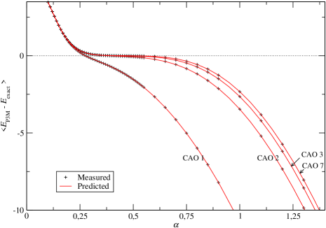
Figure 1: Comparison between the measured systematic error of the uncorrected P3M energies (crosses) and the theoretical prediction $-E_{\mathrm{P3M}}^{\mathrm{cut}}$ (solid lines) as a function of Ewald parameter $\alpha$. The average is performed over 1000 test systems consisting in 100 charges located at random in a box of size $L=10$. The mesh has size $M=8$ and the real-space cut-off is $r_{\mathrm{cut}}=4.95$.

Fig. 1 illustrates that the systematic errors in the uncorrected energies, which are due to cut-off and aliasing errors in the Madelung self-energies of the ions, have two different contributions of opposite sign. At small values of $\alpha$, the $r$-space cut-off error dominates and leads to an overestimation of the energy because the negative interaction energy of an ion with the neutralizing background charge provided by the other particles is not fully taken into account. The cut-off correction (27) derived in Sec. III does compensate very well for this effect. At large values of $\alpha$, $k$-space cut-off and aliasing errors dominate, and lead to an underestimation of the Madelung self-energies (expression (46) is indeed always negative).

Since the systematic error $\langle E^{(k)}_{\mathrm{P3M}}-E^{(k)}_{\rm exact}\rangle$ in the reciprocal energies arise solely from self terms (the Ewald interaction between a pair of particles is zero on average), this error can alternatively, and more efficiently, be measured by computing the P3M energy of a system made up of a single ion in the box, averaging that energy over different positions of the particle relative to the mesh. To restore electro-neutrality, the interaction energy (13) with the (implicit) neutralizing background must of course be taken into account before comparing the result with the exact Madelung self-energy $q^{2}\zeta/2$ of the ion. This method allows one to measure very rapidly the reciprocal contribution to the average error in the Madelung self-energies of the ions. We stress that the numerical results shown in Fig. 1 can easily be transposed to any cubic system with an arbitrary number of ions since the energy shift $E_{\mathrm{P3M}}^{\mathrm{cut}}$ scales merely as $Q^{2}/L$.

Having validated the energy shift (47), we test now the accuracy of the RMS error estimate (61). We show in Fig. 2 the theoretical predictions for the RMS error of the corrected P3M energies for different mesh sizes (thick solid lines), at fixed CAO 2. The dominant error at small values of $\alpha$ comes from the truncation in the real-space calculation, while $k$-space cut-off and aliasing errors dominate at large values of $\alpha$. The plot shows also separately the contribution $\Delta E^{(k)}_{\rm self}$, which accounts for fluctuating errors in the $k$-space Madelung self-energies, and the contribution $\Delta E^{(k)}_{\rm int}$ which accounts for fluctuating errors in the P3M pair interaction energies. Near the optimal value of $\alpha$, the error $\Delta E^{(k)}_{\mathrm{int}}$ dominates slightly $\Delta E^{(k)}_{\rm self}$ by half an order of magnitude. This validates the use of the optimal influence function (63), which was designed to minimize errors in the pair P3M interaction energies only. Notice that $\Delta E^{(k)}_{\mathrm{self}}$ overcomes $\Delta E^{(k)}_{\mathrm{int}}$ at large values of $\alpha$, in agreement with the scaling with $\alpha$ discussed in Sec. VI. The errors in Madelung self-energies must therefore by included to predict correctly the full RMS error curve in our test system with 100 charged particles, but they are expected to become negligible when the number of ions is increased above a few hundred.

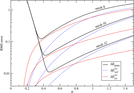
Figure 2: Theoretical predictions for the RMS error of the corrected P3M energies for CAO 2 and three different mesh sizes [thick solid lines], for the same system and real-space cut-off as in Fig. 1. The two contributions which make up the total $k$-space error are also shown independently: RMS error in the pair P3M interaction energies (Eq. (58), thin solid line) and RMS error in the Madelung self-energies (Eq. (55), dashed line).

The predicted RMS errors agree very well with the measured RMS errors, as shown in Fig. 3. The small deviations at low values of $\alpha$ are due to a loss of accuracy of Kolafa and Perram’s $r$-space error estimate (14), and to the fact that this error estimate does not take into account the improvement in accuracy brought by the new cut-off correction term (27). In the regime where the dominant error comes from the $k$-space calculation, the agreement with our RMS error estimate is excellent, especially at high values of the charge assignment order. The errors in the $k$-space calculation are caused by truncation and aliasing effects. The aliasing errors can be reduced by increasing the charge assignment order, but the accuracy cannot go below the minimum $k$-space cut-off error (67) (dashed curve in Fig. 3), which is intrinsic to the mesh size and choice of reciprocal interaction.

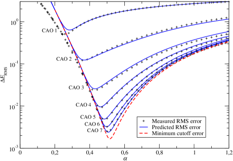
Figure 3: Comparison between the measured (crosses) and predicted (solid lines) RMS errors of the (corrected) P3M energies, for the same test system, mesh size and real-space cut-off as in Fig. 1. The minimal error due to direct and reciprocal space cut-offs is shown as a dashed line.

The pronounced minimum in the RMS error curves stresses the importance of using the optimal value of $\alpha$ when performing simulations with the P3M algorithm (or with the other variants of mesh based Ewald sums). Our accurate RMS error estimate for the P3M energies can be used to quickly find the optimal set of parameters (mesh size, charge assignment order, Ewald splitting parameter) that lead to the desired accuracy with a minimum of computational effort DH2 . Whatever the chosen parameters, it can serve also as a valuable indicator of the accuracy of the P3M energies.

VIII Conclusions

In this article, we discussed in detail which ingredients are necessary to utilize the P3M algorithm to compute accurate Coulomb energies of point charge distributions. The usage of a nearly linear scaling method ($\approx N\log N$) like P3M is almost compulsory for systems containing more than a few thousand charges.

In particular, we derived the cut-off corrections for the standard Ewald sum transparently and interpreted the systematic errors in terms of Madelung energies. This route lead us to an additional real-space cut-off correction term that has so far not been discussed in the literature. Building on these results, we have deduced the $k$-space cut-off correction term in the case of the P3M algorithm, where additional aliasing errors play a role. Furthermore we derived the exact form of the influence function that minimizes the RMS errors in the energies, and showed that this function is not much different from the force-optimized influence function, which a posteriori justifies why in most P3M implementations the usage of the force-optimized influence function does not lead to inaccurate results. Based on the energy optimized influence function we derive an accurate RMS error estimate for the energy, and performed numerical tests on sample configurations that demonstrate the validity of our error estimates and the necessity to include our correction terms. We also demonstrated that the electrostatic energy of an individual particle in the system can be obtained in the P3M method, but at the expense of an additional inverse fast Fourier transform.

With the help of the newly derived error estimates we can easily tune the desired accuracy of the P3M algorithm and find suitable parameter combinations before running any simulation.

The P3M algorithm can be generalized along our discussed lines to compute other long range interactions. Of particular interest are dipolar energies, forces and torques, and the associated error estimates for these quantities. This will be the content of a forthcoming publication. Our P3M generalization for the energies will be included in a future version of the molecular simulation package Espresso limbach06a , that is freely available under the GNU general public license. The website http://www.espresso.mpg.de provides up-to-date information.

Appendix A Ewald pair potential and Madelung self-energy

The Ewald formula for the electrostatic energy $E$ of a periodic charged system can be written in a form that underlines the fact that $E$ includes the Madelung self-energies $Q^{2}\zeta/2$ of the ions [$Q^{2}=\sum_{i}q_{i}^{2}$ and $\zeta$ is defined in (23)]. We recall from Sec. II that the Ewald formula for $E$ reads, if the system is globally neutral and if we employ metallic boundary conditions,

$$E=\frac{1}{2}\sum_{i,j}\sideset{}{{}^{{}^{\prime}}}{\sum}_{\boldsymbol{n}\in\mathbb{Z}^{3}}q_{i}q_{j}\psi(\boldsymbol{r}_{ij}+\boldsymbol{n}L)+\frac{1}{2L^{3}}\sum_{i,j}q_{i}q_{j}\sum_{\begin{subarray}{c}\boldsymbol{k}\in\mathbb{K}\\ \boldsymbol{k}\neq 0\end{subarray}}e^{-i\boldsymbol{k}\cdot(\boldsymbol{r}_{i}-\boldsymbol{r}_{j})}\widetilde{\phi}(\boldsymbol{k})-Q^{2}\frac{\alpha}{\sqrt{\pi}}.$$ (68)

The “self-energy terms” in $E$, i.e. term $E^{(s)}$ and terms $i=j$, are

$$\frac{Q^{2}}{2}\Big{(}\sum_{\boldsymbol{n}\neq 0}\psi(\boldsymbol{n}L)+\frac{1}{L^{3}}\sum_{\boldsymbol{k}\neq 0}\widetilde{\phi}(\boldsymbol{k})-\frac{2\alpha}{\sqrt{\pi}}\Big{)}=\frac{Q^{2}}{2}\Big{(}\zeta+\frac{\pi}{\alpha^{2}L^{3}}\Big{)}.$$ (69)

We can write therefore

$$E =\frac{1}{2}\sum_{i\neq j}q_{i}q_{j}\Big{(}\sum_{\boldsymbol{n}\neq 0}\psi(\boldsymbol{r}_{ij}+\boldsymbol{n}L)+\frac{1}{L^{3}}\sum_{\boldsymbol{k}\neq 0}e^{-i\boldsymbol{k}\cdot\boldsymbol{r}_{ij}}\widetilde{\phi}(\boldsymbol{k})\Big{)}+\frac{Q^{2}}{2}\Big{(}\zeta+\frac{\pi}{\alpha^{2}L^{3}}\Big{)}$$

$$=\frac{1}{2}\sum_{i\neq j}q_{i}q_{j}V_{\mathrm{Ewald}}(\boldsymbol{r}_{ij})+\frac{Q^{2}}{2}\zeta$$ (70)

where we defined the Ewald pair interaction deLeeuw

$$V_{\mathrm{Ewald}}(\boldsymbol{r})=\sum_{\boldsymbol{n}\neq 0}\psi(\boldsymbol{r}+\boldsymbol{n}L)+\frac{1}{L^{3}}\sum_{\boldsymbol{k}\neq 0}e^{-i\boldsymbol{k}\cdot\boldsymbol{r}}\widetilde{\phi}(\boldsymbol{k})-\frac{\pi}{\alpha^{2}L^{3}}.$$ (71)

Notice that in writing (70), we used $\sum_{i}\sum_{j\neq i}q_{i}q_{j}\,\pi/(\alpha^{2}L^{3})=-Q^{2}\,\pi/(\alpha^{2}L^{3})$ which follows from electro-neutrality. Thanks to the inclusion of this constant in the definition of $V_{\mathrm{Ewald}}(\boldsymbol{r})$, the Ewald pair potential does not depend on the parameter $\alpha$ [$\partial/\partial\alpha\,V_{\mathrm{Ewald}}(\boldsymbol{r})=0$] and its average over the simulation box is zero Hummer98 :

$$\left\langle{V_{\mathrm{Ewald}}(\boldsymbol{r})}\right\rangle=\frac{1}{L^{3}}\int_{L^{3}}\hbox{d}^{3}\boldsymbol{r}\,V_{\mathrm{Ewald}}(\boldsymbol{r})=0.$$ (72)

The latter property is simply a consequence of $\left\langle{\exp(i\boldsymbol{k}\cdot\boldsymbol{r}_{ij})}\right\rangle=\delta_{\boldsymbol{k},\boldsymbol{0}}$ and Eq. (21).

In conclusion, expression (70) shows explicitly that the electrostatic energy of a periodic charged system includes the Madelung self-energies $Q^{2}\zeta/2$ of the ions Brush ; Nijboer . The fact that the Ewald interaction between a pair of particles averages to zero when one particle explores the whole simulation box is also noteworthy aspect of Ewald potential Hummer98 .

Appendix B Proof of Eq. (40)

Eq. (40) is a consequence of the Sampling theorem [refs] and is straightforward to demonstrate. The sum in (32) is rewritten as an integral

$$\widetilde{\rho}_{\text{\footnotesize M}}(\boldsymbol{k})=h^{3}\int\hbox{d}\boldsymbol{r}^{\prime}\int_{V}\hbox{d}\boldsymbol{r}\,\textcyr{W}(\boldsymbol{r})U(\boldsymbol{r}-\boldsymbol{r}^{\prime})\rho(\boldsymbol{r}^{\prime})e^{-i\boldsymbol{k}\cdot\boldsymbol{r}}$$ (73)

where we used (30) and introduced an infinite mesh of Dirac delta functions

$$\textcyr{W}(\boldsymbol{r})=\sum_{\boldsymbol{r}_{m}\in\mathbb{M}_{\mathrm{p}}}\delta(\boldsymbol{r}-\boldsymbol{r}_{m})=\frac{1}{h^{3}}\sum_{\boldsymbol{m}\in\mathbb{Z}^{3}}e^{-ik_{g}\boldsymbol{m}\cdot\boldsymbol{r}}.$$ (74)

(We recall that $k_{g}=2\pi/h$). Using the above representation of $\textcyr{W}(\boldsymbol{r})$ and introducing in (73) the Fourier series representation of the periodic charge density,

$$\rho(\boldsymbol{r}^{\prime})=\frac{1}{L^{3}}\sum_{\boldsymbol{k}^{\prime}\in\mathbb{K}}\widetilde{\rho}(\boldsymbol{k}^{\prime})\,\exp(i\boldsymbol{k}^{\prime}\cdot\boldsymbol{r}^{\prime}),$$ (75)

we recover the result (40) after straightforward simplifications.

Appendix C Proof of equivalence between Eqs. (38) and (35)

Eq. (38) is equivalent to

$$E^{(ks)}_{\mathrm{P3M}}=\frac{1}{2V}\sum_{\begin{subarray}{c}\boldsymbol{k}\in\mathbb{K}\\ \boldsymbol{k}\neq 0\end{subarray}}\widetilde{\rho}^{*}(\boldsymbol{k})\widetilde{\Phi}(\boldsymbol{k}),$$ (76)

where $\widetilde{\Phi}(\boldsymbol{k})$ is the full Fourier transform ($\boldsymbol{k}\in\mathbb{K}$) of the back-interpolated potential mesh (37):

$$\widetilde{\Phi}(\boldsymbol{k})=\int_{V}\Phi(\boldsymbol{r})\hbox{d}\boldsymbol{r}=h^{3}\int_{V}\hbox{d}\boldsymbol{r}\,e^{-i\boldsymbol{k}\cdot\boldsymbol{r}}\int\hbox{d}\boldsymbol{r}^{\prime}\textcyr{W}(\boldsymbol{r}^{\prime})U(\boldsymbol{r}-\boldsymbol{r}^{\prime})\Phi_{\text{\footnotesize M}}(\boldsymbol{r}^{\prime}).$$ (77)

We replace in this equation $\Phi_{\text{\footnotesize M}}(\boldsymbol{r}^{\prime})$ and $\textcyr{W}(\boldsymbol{r}^{\prime})$ by their expressions (36) and (74), and perform the integration over $\boldsymbol{r}^{\prime}$:

$$\widetilde{\Phi}(\boldsymbol{k})=\frac{1}{L^{3}}\sum_{\boldsymbol{k}^{\prime}\in\widetilde{\mathbb{M}}}\widetilde{\Phi}_{\text{\footnotesize M}}(\boldsymbol{k}^{\prime})\sum_{\boldsymbol{m}}\int_{V}\hbox{d}\boldsymbol{r}\,e^{-i\boldsymbol{k}\cdot\boldsymbol{r}}\,\widetilde{U}(\boldsymbol{k}^{\prime}+k_{g}\boldsymbol{m})e^{i(\boldsymbol{k}^{\prime}+k_{g}\boldsymbol{m})\cdot\boldsymbol{r}}.$$ (78)

The integration over $\boldsymbol{r}$ introduces a Kronecker symbol $\delta_{\boldsymbol{k},\boldsymbol{k}^{\prime}+k_{g}\boldsymbol{m}}$. We get therefore the simple result

$$\widetilde{\Phi}(\boldsymbol{k})=\widetilde{\Phi}_{\text{\footnotesize M}}(\boldsymbol{k})\widetilde{U}(\boldsymbol{k})$$ (79)

where the function $\widetilde{\Phi}_{\text{\footnotesize M}}(\boldsymbol{k})$, which is defined originally only for $\boldsymbol{k}\in\widetilde{\mathbb{M}}$, is now understood to be extended periodically to all $\mathbb{K}$ space. Notice that the inverse FFT does not introduce aliasing errors: the sum over $\boldsymbol{m}$ merely renders $\widetilde{\Phi}_{\text{\footnotesize M}}(\boldsymbol{k})$ periodic. In accordance with (32) and (34), we extend also $\widetilde{\rho}_{\text{\footnotesize M}}(\boldsymbol{k})$ and $\widetilde{G}(\boldsymbol{k})$ periodically, with period $2\pi/h$. Using the above result and (34), the reciprocal energy (76) can be expressed as

$$E^{(ks)}_{\mathrm{P3M}} =\frac{1}{2L^{3}}\sum_{\boldsymbol{k}\in\mathbb{K}}\widetilde{\rho}^{*}(\boldsymbol{k})\widetilde{U}(\boldsymbol{k})\widetilde{\rho}_{\text{\footnotesize M}}(\boldsymbol{k})\widetilde{G}(\boldsymbol{k})$$ (80)

$$=\frac{1}{2L^{3}}\sum_{\boldsymbol{k}\in\widetilde{\mathbb{M}}}\sum_{\boldsymbol{m}\in\mathbb{Z}^{3}}\widetilde{\rho}^{*}(\boldsymbol{k}+k_{g}\boldsymbol{m})\widetilde{U}(\boldsymbol{k}+k_{g}\boldsymbol{m})\widetilde{\rho}_{\text{\footnotesize M}}(\boldsymbol{k})\widetilde{G}(\boldsymbol{k}).$$ (81)

This may be compared with Eq. (35), i.e.

$$E^{(ks)}_{\mathrm{P3M}}=\frac{1}{2L^{3}}\sum_{\begin{subarray}{c}\boldsymbol{k}\in\widetilde{\mathbb{M}}\\ \boldsymbol{k}\neq 0\end{subarray}}\widetilde{\rho}_{\text{\footnotesize M}}^{*}(\boldsymbol{k})\widetilde{\rho}_{\text{\footnotesize M}}(\boldsymbol{k})\widetilde{G}(\boldsymbol{k}).$$ (82)

Recalling (40) and the fact that $\widetilde{U}(\boldsymbol{k})$ is real, we see that both expressions are equivalent.

References

• (1) A. Arnold and C. Holm,in Advanced Computer Simulation Approaches for Soft Matter Sciences II, eds. C. Holm and K. Kremer (Springer, Berlin, 2005)
• (2) R.W. Hockney and J.W. Eastwood, Computer Simulation Using Particles (IOP, Bristol, 1988)
• (3) M. Deserno and C. Holm, J. Chem. Phys. 109 (1998): 7678
• (4) U. Essmann, L. Perera et al., J. Chem. Phys. 103 (1995): 8577
• (5) M. Deserno and C. Holm, J. Chem. Phys. 109 (1998): 7694
• (6) S.W. de Leeuw, J.W. Perram and E.R. Smith, Proc. R. Soc. London, Ser. A 373 (1980):57
• (7) J.-M. Caillol, J. Chem. Phys. 101 (1994): 6080
• (8) E.R. Smith, Mol. Phys. 65 (1988): 1089
• (9) V. Ballenegger and J.-P. Hansen, J. Chem. Phys. 122 (2005): Art. 114711
• (10) J. Kirkwood, J. Chem. Phys. 7 (1939): 911
• (11) A. Alastuey and V. Ballenegger, Physica A 279 (2000): 268
• (12) V. Ballenegger and J.-P. Hansen, Mol. Phys. 102 (2004): 599
• (13) P. Ewald, Ann. Phys. (Leipzig) 64 (1921): 253
• (14) G. Hummer, L.R. Pratt and A.E. García, J. Phys. Chem. 99 (1995):14188
• (15) M.P. Allen and D.J. Tildesley, Computer Simulation of Liquids Oxford Science Publications. (Clarendon Press, Oxford, 1987)
• (16) J. Kolafa and J.W. Perram, Mol. Sim. 9 (1992): 351
• (17) S.G. Brush, H.L. Sahlin and E. Teller, J. Chem. Phys. 45 (1966): 2102
• (18) B.R. Nijboer and T.W. Ruijgrok, J. Stat. Phys. 53 (1988): 361
• (19) T. Darden, D. Pearlman and L.G. Pedersen, J. Chem. Phys. 109 (1998): 10921
• (20) Z. Wang and C. Holm, J. Chem. Phys. 115 (2001): 6351
• (21) H.J. Limbach, A. Arnold, B.A. Mann, and C. Holm, Comp. Phys. Comm. 174, (2006): 704
• (22) G. Hummer, L.R. Pratt and A.E. García, J. Phys. Chem. A 102 (1998):7885