Effective Theory Approach to
$W$-Pair Production near Threshold

Abstract

In this talk, I review the effective theory approach to unstable particle production and present results of a calculation of the process $e^{-}e^{+}\rightarrow\mu^{-}\bar{\nu}_{\mu}u\bar{d}\,X$ near the $W$-pair production threshold up to next-to-leading order in $\Gamma_{W}/M_{W}\sim\alpha\sim v^{2}$. The remaining theoretical uncertainty and the impact on the measurement of the $W$ mass is discussed.

SFB/CPP-07-44, arXiv:0708.0730 [hep-ph], August 6, 2007

1 Introduction

The masses of particles like the top quark, the $W$ boson or yet undiscovered particles like supersymmetric partners can be measured precisely using threshold scans at an $e^{-}e^{+}$ collider. In particular the error of the $W$ mass could be reduced to $6\,$MeV by measuring the four fermion production cross section near the $W$-pair threshold [1], provided theoretical uncertainties are reduced well below $1\%$. In such precise calculations one has to treat finite width effects systematically and without violating gauge invariance. The next-to-leading order (NLO) calculations of $W$-pair production [2] available at LEP2 were done in the pole scheme [3] and were supposed to break down near threshold. The recent computation of the complete NLO corrections to $e^{-}e^{+}\to 4f$ processes in the complex mass scheme [4] is valid near threshold and in the continuum, but is technically demanding and required to compute one loop six-point functions.

In this talk, I report on the NLO corrections to the total cross section of the process

$$e^{-}e^{+}\to\mu^{-}\bar{\nu}_{\mu}u\bar{d}X$$ (1)

near the $W$-pair threshold [5] obtained using effective field theory (EFT) methods [6, 7, 8]. This calculation is simpler than the one of [4] and results in an almost analytical expression of the result that allows for a detailed investigation of theoretical uncertainties. However, the method is not easily extended to differential cross sections. Section 2 contains the leading order (LO) EFT description while the NLO approximation of the tree and the radiative corrections are described in Sections 3 and 4, respectively. Results are presented in Section 5 together with an estimate of the remaining theoretical uncertainties and a comparison to [4].

2 Unstable particle effective theory

To provide a systematic treatment of finite width effects, in [6, 7] EFT methods were used to expand the cross section simultaneously in the coupling constant $\alpha$, the ratio $\Gamma/M$ and the virtuality of the resonant particle $(k^{2}-M^{2})/M^{2}$, denoted collectively by $\delta$. The modes at the small scale $\delta$ (the resonance, soft or Coulomb photons, …) and the external particles are described by an effective Lagrangian $\mathcal{L}_{\text{eff}}$ that contains elements of heavy quark effective theory or non-relativistic QED and soft-collinear effective theory (SCET) (for reviews of the various EFTs see e.g [10]). “Hard” fluctuations with virtualities $\sim M^{2}$ are not part of the EFT and are integrated out. Their effect is included in short-distance coefficients in $\mathcal{L}_{\text{eff}}$ that can be computed in fixed-order perturbation theory without resummations of self-energies. Finite width effects are relevant for the modes at the small scale and are incorporated through complex short-distance coefficients in $\mathcal{L}_{\text{eff}}$  [7, 9].

It might be useful to compare the EFT approach to the pole scheme for the example of the production of a single resonance $\Phi$ in the inclusive process $f_{1}\bar{f}_{2}\to X$. The pole scheme provides a decomposition of the amplitude into resonant and non-resonant pieces [3]:

$$\mathcal{A}(s)|_{s\sim M^{2}}=\frac{\mathcal{R}(\bar{s})}{s-\bar{s}}+\mathcal{N}(s),$$ (2)

where both $\bar{s}$, the complex pole of the propagator defined by $\bar{s}-M^{2}-\Pi(\bar{s})=0$, and $\mathcal{R}(\bar{s})$, the residue of $\mathcal{A}(s)$ at $\bar{s}$, are gauge independent. In the EFT, it is convenient to obtain the cross section from the imaginary part of the forward-scattering amplitude that reads [7]

$$i\mathcal{A}(s)|_{s\sim M^{2}}=\int d^{4}x\,\langle f_{1}\bar{f}_{2}|T\left[i{\cal O}^{\dagger}_{\Phi f_{1}\bar{f}_{2}}(0)i{\cal O}_{f_{1}\bar{f}_{1}\Phi}(x)\right]|f_{1}\bar{f}_{2}\rangle+\langle f_{1}\bar{f}_{2}|i{\cal O}_{4f}(0)|f_{1}\bar{f}_{2}\rangle\,.$$ (3)

Here ${\cal O}_{f_{1}\bar{f}_{2}\Phi}$ describes the production of $\Phi$ while ${\cal O}_{4f}$ describes non-resonant contributions. The matching coefficients of these operators are gauge independent since they are computed from on-shell scattering amplitudes in the underlying theory, where for unstable particles “on-shell” implies $k^{2}=\bar{s}$. The structure of (3) is similar to (2), but the EFT provides a field theoretic definition of the several terms. Higher order corrections to the matching coefficients correspond to the factorizable corrections in the pole scheme. Loop corrections to the matrix elements in the EFT correspond to the non-factorizable corrections [6].

Turning to $W$-pair production near threshold, the appropriate effective Lagrangian to describe the two non-relativistic $W$ bosons with $k^{2}-M_{W}^{2}\sim M_{W}^{2}v^{2}\sim M_{W}^{2}\delta$ is given by [8]

$${\cal L}_{\rm NRQED}=\sum_{a=\mp}\left[\Omega_{a}^{\dagger i}\left(iD^{0}+\frac{\vec{D}^{2}}{2{M}_{W}}-\frac{\Delta}{2}\right)\Omega_{a}^{i}+\Omega_{a}^{\dagger i}\,\frac{(\vec{D}^{2}-M_{W}\Delta)^{2}}{8M_{W}^{3}}\,\Omega_{a}^{i}\right]$$ (4)

with the matching coefficient [7] $\Delta\equiv(\bar{s}-M_{W}^{2})/M_{W}$. If $M_{W}$ is the pole mass, this becomes $\Delta=-i\Gamma_{W}$. The fields $\Omega^{i}_{\pm}\equiv\sqrt{2M_{W}}W^{i}_{\pm}$ describe the three physical polarizations of the $W$s; the unphysical modes are not part of the EFT [8]. The covariant derivative $D_{\mu}\Omega_{\pm}^{i}\equiv(\partial_{\mu}\mp ieA_{\mu})\Omega_{\pm}^{i}$ includes interactions with those photon fluctuations that keep the virtualities of the $\Omega$s at the order $\delta$. These are soft photons with $(q^{0},\vec{q})\sim(\delta,\delta)$ and potential (Coulomb) photons with $(q^{0},\vec{q})\sim(\delta,\sqrt{\delta})$. Collinear photons are also part of the EFT but do not contribute at NLO. The Lagrangian (4) reproduces the expansion of the resummed transverse $W$ propagator in $\delta$, as can be seen by writing the $W$ four-momenta as $k^{\mu}=M_{W}\,v^{\mu}+r^{\mu}$ with $v^{\mu}\equiv(1,\vec{0})$ and a potential residual momentum $(r^{0},|\vec{r}|)\sim M_{W}\,(v^{2},v)\sim(\delta,\sqrt{\delta})$:

$$\frac{i}{k^{2}-M_{W}^{2}-\Pi^{W}_{T}(k^{2})}\left(-g_{\mu\nu}+\frac{k_{\mu}k_{\nu}}{k^{2}}\right)\qquad\Rightarrow\qquad\frac{i(-g_{\mu\nu}+v_{\mu}v_{\nu})}{2M_{W}(r^{0}-\frac{{\vec{r}}^{2}}{2M_{W}}+\frac{\Delta}{2})}\,.$$ (5)

Higher orders in the expansion of the propagator are reproduced by the higher order kinetic terms in (4) and residue factors included in the production operators [5].

The production of a pair of non-relativistic $W$ bosons is described by the operator [8]

$${\cal O}_{p}^{(0)}=\frac{\pi\alpha}{s_{w}^{2}M_{W}^{2}}\left(\bar{e}_{c_{2},L}\left(\gamma^{i}n^{j}+\gamma^{j}n^{i}\right)e_{c_{1},L}\right)\left(\Omega_{-}^{\dagger i}\Omega_{+}^{\dagger j}\right)$$ (6)

that is determined from the on-shell tree-level scattering amplitude $e^{-}e^{+}\to W^{+}W^{-}$:

$$\parbox{256.0748pt}{ \includegraphics[height=41.25648pt]{wtalk-figs-1.eps} }\,.$$ (7)

At threshold, only the $t$-channel diagram and the $e^{-}_{L}e^{+}_{R}$ helicity contribute at leading order in $\delta$. Similar to (3), the LO $e^{-}e^{+}$ forward-scattering amplitude in the EFT is given by the expectation value of a time ordered product of the operators (6), evaluated using (4):

$$i{\cal A}^{(0)}=\int d^{4}x\,\langle e^{-}e^{+}|{\mathrm{T}}[i{\cal O}_{p}^{(0)\dagger}(0)i{\cal O}_{p}^{(0)}(x)]|e^{-}e^{+}\rangle=\parbox{73.97716pt}{ \includegraphics[height=44.10176pt]{wtalk-figs-2.eps} }\,.$$ (8)

One estimates ${\cal A}^{(0)}\sim\alpha^{2}\sqrt{\delta}$, noting that each $\Omega$ propagator (5) contributes $\delta^{-1}$ and counting the potential loop integral as $dk^{0}d^{3}k_{i}\sim\delta^{5/2}$. The total cross section for the process (1) is obtained from appropriate cuts of ${\cal A}^{(0)}$, where cutting an $\Omega_{\pm}$ line has to be interpreted as cutting the self-energies resummed in the EFT propagator. At LO, the cuts contributing to the flavour-specific final state are correctly extracted by multiplying the imaginary part of ${\cal A}^{(0)}$ by the leading-order branching fractions. In terms of $E=\sqrt{s}-2M_{W}$ one obtains [5]

$$\sigma^{(0)}(e^{-}e^{+}\to\mu^{-}\bar{\nu}_{\mu}u\bar{d})=\frac{\pi\alpha^{2}}{27s_{w}^{4}s}\text{Im}\left[-i\,\sqrt{-\frac{E+i\Gamma_{W}}{M_{W}}}\;\right]\,.$$ (9)

3 NLO EFT approximation to the born cross section

Some parts of the NLO EFT calculation of the process (1) are included in a Born calculation in the full theory with a fixed width prescription. One contribution arises from four-electron operators ${\cal O}^{(k)}_{4e}$ analogous to those in (3). Their matching coefficients $C^{(k)}_{4e}$ are obtained from the forward-scattering amplitude in the full electroweak theory. The leading imaginary parts of $C^{(k)}_{4e}$ are of order $\alpha^{3}$ and arise from cut two-loop diagrams corresponding to all squared tree diagrams of the processes $e^{-}e^{+}\to W^{-}u\bar{d}$ and $e^{-}e^{+}\to W^{+}\mu^{-}\bar{\nu}_{\mu}$, calculated in dimensional regularization without self-energy resummations, but expanded near threshold:

(10)

Since these corrections to the amplitude are of order $\alpha^{3}$, and counting $\alpha\sim\delta$, they are suppressed by $\delta^{1/2}$ compared to ${\cal A}^{(0)}\sim\alpha^{2}\delta^{1/2}$ and are denoted as ”$\sqrt{\mathrm{N}}$LO” corrections.

The second class of contributions arises from production-operator and propagator corrections. Performing the tree-level matching (7) up to order $\sim v$ and $v^{2}$ leads to higher order production operators ${\cal O}_{p}^{(1/2)}$ and ${\cal O}_{p}^{(1)}$. The operators ${\cal O}_{p}^{(1/2)}$ like $\left(\bar{e}_{L}\gamma^{j}e_{L}\right)\left(\Omega_{-}^{i}(-i)D^{j}\Omega_{+}^{i}\right)$ are given in [8]. At NLO one needs diagrams with two insertions of an ${\cal O}_{p}^{(1/2)}$ operator, one insertion of an ${\cal O}_{p}^{(1)}$ operator and insertions of kinetic corrections from (4):

$$i{\cal A}^{(1)}_{\text{born}}=\parbox{256.0748pt}{ \includegraphics[height=52.63759pt]{wtalk-figs-4.eps}}$$

Equivalently one can directly expand the spin averaged squared matrix elements [5].

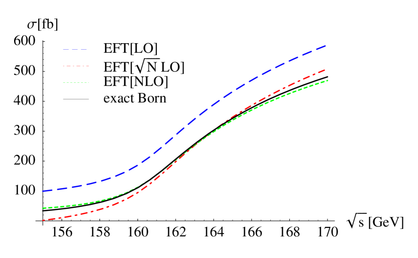
Figure 1: Convergence of EFT approximations to the born cross section from Whizard

As seen in Figure 1, the EFT approximations converge to the full Born result but it turns out that a partial inclusion of N^3/2LO corrections is required to get an agreement of $\sim 0.1\%$ at 170 GeV and $\sim 10\%$ at 155 GeV [5]. For higher-order initial state radiation (ISR) improvement by a convolution with radiator functions, one needs $\sigma_{\text{Born}}$ at energies far below threshold, where the EFT is not valid. For the numerical results in Section 5 the ISR-improved Born cross section from Whizard [11] was used, but one could also match the EFT to the full theory below, say, $\sqrt{s}=155$ GeV.

4 Radiative corrections

The radiative corrections needed up to NLO are given by higher order calculations of short distance coefficients and by loop calculations in the EFT. Counting the QCD coupling constant as $\alpha_{s}^{2}\sim\alpha_{ew}\sim\delta$, the corrections to $\Gamma_{W}$ up to order $\alpha_{ew}\alpha_{s}$ ($\sqrt{\text{N}}$LO), $\alpha_{ew}^{2}$ and $\alpha_{ew}\alpha_{s}^{2}$ (NLO) have to be included. The flavour-specific NLO decay corrections are correctly taken into account by multiplying the imaginary part of the LO forward-scattering amplitude with the one-loop corrected branching ratios. For the NLO renormalization of the production operator (6) one has to calculate the one-loop corrections to the on-shell scattering $e^{-}e^{+}\to W^{+}W^{-}$ at leading order in the non-relativistic expansion:

Due to the threshold kinematics, many of the 180 one-loop diagrams do not contribute, consistent with the vanishing of the tree-level $s$-channel diagrams at leading order in $v$. In terms of a finite coefficient $c_{p}^{(1,{\rm fin})}$ given in [5], the matching coefficient reads

$$C_{p}^{(1)}=\frac{\alpha}{2\pi}\left[\left(-\frac{1}{\varepsilon^{2}}-\frac{3}{2\varepsilon}\right)\left(-\frac{4M_{W}^{2}}{\mu^{2}}\right)^{-\varepsilon}+c_{p}^{(1,{\rm fin})}\right]\,.$$ (11)

The first and second Coulomb correction arise from the exchange of potential photons. Their magnitude can be estimated counting the loop-integral measure in the potential region as $d^{4}q\sim\delta^{5/2}$, the $\Omega$ propagator and the potential photon propagator $i/|\vec{q}|^{2}$ as $\delta^{-1}$. One finds that single Coulomb exchange is a $\sqrt{\text{N}}$LO correction compared to the LO amplitude:

$$\parbox{62.59605pt}{ \includegraphics[height=42.67912pt]{wtalk-figs-6.eps} }\sim\alpha^{3}\int d^{4}k\;d^{4}q\;\frac{1}{|\vec{q}|^{2}}\;\delta^{-4}\;\sim\;\alpha^{3}\;\sim{\cal A}^{(0)}\sqrt{\delta}$$ (12)

At threshold the one-photon exchange is of the order of 5% of the LO amplitude while two-photon exchange is only a few-permille correction [12] and no resummation is necessary.

Soft photon corrections correspond to two-loop diagrams in the EFT containing a photon with momentum $(q_{0},|\vec{q}\,|)\sim(\delta,\delta)$. They give rise to $\mathcal{O}(\alpha)$ corrections as can be seen from a power-counting argument similar to the one for Coulomb-exchange but counting the soft-photon propagator $-i/q^{2}$ as $\delta^{-2}$ and the soft loop-integral as $\delta^{4}$. In agreement with gauge invariance arguments and earlier calculations [13], the sum of all diagrams where a soft photon couples to an $\Omega$ line vanishes. The only remaining diagrams give

$$\parbox{105.27519pt}{ \includegraphics[height=42.67912pt]{wtalk-figs-7.eps} }\quad=\frac{4\pi^{2}\alpha^{2}}{s_{w}^{4}M_{W}^{2}}\frac{\alpha}{\pi}\int\frac{d^{d}r}{(2\pi)^{d}}\frac{1}{\eta_{-}\eta_{+}}\left[\left(\frac{1}{\varepsilon^{2}}+\frac{5}{12}\pi^{2}\right)\left(-\frac{2\eta_{-}}{\mu}\right)^{-2\varepsilon}\right]$$ (13)

with $\eta_{-}=r_{0}-\frac{|\vec{r}|^{2}}{2M_{W}}+i\frac{\Gamma^{(0)}}{2}$ and $\eta_{+}=E-r_{0}-\frac{|\vec{r}|^{2}}{2M_{W}}+i\frac{\Gamma^{(0)}}{2}$. The $\epsilon^{-2}$ poles cancel between (13) and diagrams with an insertion of the NLO production operator (11) while the remaining $\epsilon^{-1}$ poles proportional to $\left(2\log\left(\eta_{-}/M_{W}\right)+3/2\right)$ are discussed below.

5 Results and estimate of remaining uncertainties

The radiative corrections in Section 4 were calculated for $m_{e}=0$ so the result is not infrared safe. It should be convoluted with electron distribution functions in the $\overline{\text{MS}}$ scheme after minimal subtraction of the IR poles. However, the available distribution functions assume $m_{e}$ as IR regulator. Our result can be converted to this scheme by adding contributions from the hard-collinear region where $k^{\mu}\sim M_{W},\,k^{2}\sim m_{e}^{2}$, and the soft-collinear region where $k^{\mu}\sim\Gamma_{W},\,k^{2}\sim m_{e}^{2}\frac{\Gamma_{W}}{M_{W}}$. These cancel the $\epsilon$-poles but introduce large logs of $M_{W}/m_{e}$:

$$\sigma^{(1)}(s)=\frac{\alpha^{3}}{27s_{w}^{4}s}\,\text{Im}\Bigg{\{}(-1)\,\sqrt{-\tfrac{E+i\Gamma_{W}}{M_{W}}}\,\bigg{(}4\ln\bigg{(}-\frac{4(E+i\Gamma_{W})}{M_{W}}\bigg{)}\ln\left(\frac{2M_{W}}{m_{e}}\right)\\ -5\ln\left(\frac{2M_{W}}{m_{e}}\right)+\mbox{Re}\,\Big{[}c_{p}^{(1,\rm fin)}\Big{]}+\frac{\pi^{2}}{4}+3\bigg{)}\Bigg{\}}+\Delta\sigma^{(1)}_{\mbox{\tiny Coulomb}}+\Delta\sigma^{(1)}_{\mbox{\tiny decay}}\,.$$ (14)

At this stage, one can compare to the results of [4] for the strict $\mathcal{O}(\alpha_{ew})$ corrections without higher order ISR improvement, $\sigma_{4\text{f}}(161\text{GeV})=105.71(7)$ fb and $\sigma_{4\text{f}}(170\text{GeV})=377.1(2)$. From (14) one obtains $\sigma_{\text{EFT}}(161\text{GeV})=104.97(6)$ fb and $\sigma_{\text{EFT}}(170\text{GeV})=373.74(2)$ so the difference between the EFT and [4] is only about $0.7\%-1\%$.

The large logs in (14) can be resummed by convoluting the NLO cross section with the structure functions used e.g. in [2], after appropriate subtractions to avoid double-counting. The solid line in Figure 2 shows the resulting corrections relative to $\sigma_{\text{Born}}$. Compared to the large correction from ISR improvement of $\sigma_{\text{Born}}$ alone (blue/dashed), the size of the genuine radiative correction is about $+8\%$.

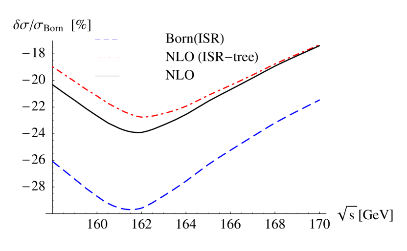
Figure 2: Size of the relative NLO corrections for different treatments of ISR

The largest remaining uncertainty is due to the treatment of ISR that is accurate only at leading-log level. It is formally equivalent to improve only $\sigma_{\text{Born}}$ by higher order ISR [2, 4], but not the radiative corrections. The results of this approach are shown in the red (dash-dotted) line in Figure 2 and differ by almost $2\%$ at threshold from the treatment discussed above. This translates to an uncertainty of $\delta M_{W}\sim 31\,\mbox{MeV}$ [5]. The remaining theory uncertainty comes from the uncalculated N^3/2LO corrections in the EFT. The $O(\alpha)$ corrections to the the four-electron operators (10) lead to an estimated uncertainty of $\delta M_{W}\sim 8$ MeV [5]. These corrections are included in [4]. The effect of diagrams with single-Coulomb exchange together with a soft photon or a hard correction to the production vertex is estimated as $\delta M_{W}\sim 5$ MeV. Therefore it should be possible to reach the theoretical accuracy required for the $M_{W}$ measurement since the largest remaining uncertainties can be eliminated by an improved treatment of ISR and with input of the full four fermion calculation.

References

- [1] G. Wilson in 2nd ECFA/DESY Study, pp. 1498–1505. Desy LC note LC-PHSM-2001-009
- [2] A. Denner, S. Dittmaier, M. Roth, and D. Wackeroth Phys. Lett. B475 (2000) 127–134, [hep-ph/9912261]; Nucl. Phys. B587 (2000) 67–117, [hep-ph/0006307]; W. Beenakker, F. A. Berends, and A. P. Chapovsky Nucl. Phys. B548 (1999) 3–59, [hep-ph/9811481]
- [3] R. G. Stuart Phys. Lett. B262 (1991) 113–119; A. Aeppli, G. J. van Oldenborgh, and D. Wyler Nucl. Phys. B428 (1994) 126–146, [hep-ph/9312212]
- [4] A. Denner, S. Dittmaier, M. Roth, and L. H. Wieders Phys. Lett. B612 (2005) 223–232, [hep-ph/0502063]; Nucl. Phys. B724 (2005) 247–294, [hep-ph/0505042]
- [5] M. Beneke, P. Falgari, C. Schwinn, A. Signer, and G. Zanderighi arXiv:0707.0773 [hep-ph]
- [6] A. P. Chapovsky, V. A. Khoze, A. Signer, and W. J. Stirling Nucl. Phys. B621 (2002) 257–302, [hep-ph/0108190]
- [7] M. Beneke, A. P. Chapovsky, A. Signer, and G. Zanderighi Phys. Rev. Lett. 93 (2004) 011602, [hep-ph/0312331]; Nucl. Phys. B686 (2004) 205–247, [hep-ph/0401002]
- [8] M. Beneke, N. Kauer, A. Signer, and G. Zanderighi Nucl. Phys. Proc. Suppl. 152 (2006) 162–167, [hep-ph/0411008]
- [9] A. H. Hoang and C. J. Reisser Phys. Rev. D71 (2005) 074022, [hep-ph/0412258]
- [10] I. Z. Rothstein, TASI lectures 2002, hep-ph/0308266; M. Neubert, TASI lectures 2004, hep-ph/0512222
- [11] W. Kilian in 2nd ECFA/DESY Study, pp. 1924–1980. DESY LC-Note LC-TOOL-2001-039
- [12] V. S. Fadin, V. A. Khoze, and A. D. Martin Phys. Lett. B311 (1993) 311–316; V. S. Fadin, V. A. Khoze, A. D. Martin, and W. J. Stirling Phys. Lett. B363 (1995) 112–117, [hep-ph/9507422]
- [13] V. S. Fadin, V. A. Khoze, and A. D. Martin Phys. Rev. D49 (1994) 2247–2256; K. Melnikov and O. I. Yakovlev Phys. Lett. B324 (1994) 217–223, [hep-ph/9302311]